


 Abstract
 HTML
HTML Reference
 Related
 PDF
PDF


-
Since the 125 GeV/
$ c^2 $ Higgs boson was discovered at the Large Hadron Collider (LHC) in 2012 [1,2], its properties have been tested increasingly precisely [3-5]. Even though no new physics beyond Standard Model (SM) has been confirmed so far, it is still necessary and meaningful to search for new physics. In this paper we study the anomalous$ HZZ $ couplings.The new physics beyond the SM in the SM effective field theory (SMEFT) is shown as higher-dimensional operators in the Lagrangian, which later supply non-SM interactions. In this analysis we note these non-SM
$ HVV $ ($ V $ represents$ Z,W,\gamma $ ) interactions from six-dimensional operators as anomalous$ HVV $ couplings, and consider them separately from SM loop contributions. To scrutinize the Lorentz structures from several anomalous couplings, we calculate the scattering amplitudes in the spinor helicity method, and the analytic formulas are shown symmetrically and elegantly in the spinor notations.$ HVV $ couplings can be probed at the LHC through processes including$ V^\ast\to VH $ or$ H\to VV $ decays. Among these processes, the$ gg\to H\to ZZ \to 4\ell $ process, which is called the golden channel, is the most precise and has been studied extensively in both theoretical studies [6-41] and experiments at LHC [42-50]. Thus, we also choose this golden channel to study anomalous$ HVV $ couplings. To reach a more precise result, both on-shell and off-shell Higgs regions can be exploited. At the same time, the interference effects between this process and the SM processes should be included. Especially in the off-shell Higgs region, the interference between this process and the continuum process$ gg\to ZZ \to 4\ell $ should not be ignored [51,52]. Based on a modified MCFM [51,53] package with anomalous$ HZZ $ couplings, we study the interference effects quantitatively. Furthermore, we estimate the constraints on the anomalous coupling using CMS experimental data at LHC.The rest of the paper is organized as follows. In Section 2, the spinor helicity amplitudes with anomalous couplings are calculated. In Section 3, the analytic formulas are embedded into the MCFM8.0 package and the cross sections for proton–proton collision, especially the interference effects, are shown numerically. In Section 4, the constraints on the
$ HZZ $ anomalous couplings are estimated. Section 5 is the discussion and conclusion. -
In this section, firstly we introduce the
$ HZZ $ anomalous couplings, and then we calculate the spinor helicity amplitudes. -
In the SM effective field theory [54,55] the complete form of higher-dimensional operators can be written as
$ {\cal{L}} = {\cal{L}}_{\rm SM}+\frac{1}{\Lambda}\sum\limits_k C_k^{5}{\cal{O}}_k^{5} +\frac{1}{\Lambda^2}\sum\limits_k C_k^{6}{\cal{O}}_k^{6}+{\cal{O}}\left(\frac{1}{\Lambda^3}\right)\; , $

(1) where
$ \Lambda $ is the new physics energy scale, and$ C_k^{i} $ with$ i = 5,6 $ are Wilson loop coefficients. As the dimension-five operators$ {\cal{O}}_k^{5} $ have no contribution to anomalous$ HZZ $ couplings, the dimension-six operators$ {\cal{O}}_k^{6} $ have leading contributions. The relative dimension-six operators in the Warsaw basis [55] are$ \begin{split}& {\cal{O}}^6_{\Phi D} = (\Phi^{\dagger}D^{\mu}\Phi)^{\ast}(\Phi^{\dagger}D^{\mu}\Phi), \\& {\cal{O}}^6_{\Phi W} = \Phi^\dagger \Phi W^{I}_{\mu\nu}W^{I\mu\nu},\; \; {\cal{O}}^6_{\Phi B} = \Phi^\dagger\Phi B_{\mu\nu}B^{\mu\nu},\\& {\cal{O}}^6_{\Phi WB} = \Phi^\dagger \tau^I \Phi W^{I}_{\mu\nu}B^{\mu\nu}, \;\; {\cal{O}}^6_{\Phi \tilde{W}} = \Phi^\dagger\Phi \tilde{W}^{I}_{\mu\nu}W^{I\mu\nu}, \\& {\cal{O}}^6_{\Phi \tilde{B}} = \Phi^\dagger\Phi \tilde{B}_{\mu\nu}B^{\mu\nu}, \; \; {\cal{O}}^6_{\Phi \tilde{W}B} = \Phi^\dagger \tau^I \Phi \tilde{W}^{I}_{\mu\nu}B^{\mu\nu}, \end{split} $

(2) where
$ \Phi $ is a doublet representation under the$ SU(2)_L $ group and the aforementioned Higgs field$ H $ is one of its four components;$D_\mu = \partial_\mu-{\rm i} g W^{I}_{\mu}T^{I}-{\rm i}g^{\prime}YB_\mu$ , where$ g $ and$ g^\prime $ are coupling constants,$ T^{I} = \tau^{I}/2 $ where$ \tau^{I} $ are Pauli matrices, and$ Y $ is the$ U(1)_Y $ generator;$W^{I}_{\mu\nu} = \partial_\mu W^{I}_{\nu}- \partial_\nu W^{I}_\mu - g\epsilon^{IJK}W^{J}_\mu W^{K}_\nu$ ,$ B_{\mu\nu} = \partial_\mu B_\nu-\partial_\nu B_\mu $ ;$ \tilde{W}^{I}_{\mu\nu} = \dfrac{1}{2}\epsilon_{\mu\nu\rho\sigma}W^ {I\rho\sigma} $ ; and$\tilde{B}_{\mu\nu} = \dfrac{1}{2}\epsilon_{\mu\nu\rho\sigma}B^ {\rho\sigma}$ .For the
$ H\to 4\ell $ process that we are going to take to constrain the anomalous$ HZZ $ couplings numerically, there are dimension-six operators including the$ HZ\ell\ell $ contact interaction [56,57] that can also contribute non-SM effects, which are$ \begin{split}& {\cal{O}}^6_{\Phi L} = (\Phi^\dagger {\overleftrightarrow D}_\mu\Phi)( \bar{L}\gamma_\mu L), \\& {\cal{O}}^6_{\Phi LT} = (\Phi^\dagger T^I {\overleftrightarrow D}_\mu \Phi)( \bar{L}\gamma_\mu T^I L), \\& {\cal{O}}^6_{\Phi e} = (\Phi^\dagger {\overleftrightarrow D}_\mu\Phi)(\bar{e}\gamma_\mu e), \end{split}$

(3) where
$\begin{aligned}& \Phi^\dagger {\overleftrightarrow D}_\mu\Phi = \Phi^\dagger D_\mu\Phi-D_\mu\Phi^\dagger\Phi,\\ &\Phi^\dagger T^I {\overleftrightarrow D}_\mu\Phi = \Phi^\dagger T^I D_\mu\Phi- D_\mu\Phi^\dagger T^I \Phi,\end{aligned}$

$ L $ ,$ e $ represent left- and right-handed charged leptons. One may worry about the pollution caused by the$ HZ\ell\ell $ contact interaction from these operators to the$ 4\ell $ final state when probing$ HZZ $ couplings. Nevertheless, we can use certain additional methods to distinguish them. In the off-shell Higgs region, the on-shell$ Z $ boson selection cut can reduce much of the$ HZ\ell\ell $ background. In the on-shell Higgs region, the non-leptonic$ Z $ decay channel can also be adopted in constraining$ HZZ $ couplings. These discussions are not the focus of the current paper and we are not going to examine them in detail here.After spontaneous symmetry breaking, we get the anomalous
$ HZZ $ interactions$ {\cal{L}}_{a} = \frac{a_1}{v}M_Z^2 HZ^{\mu}Z_{\mu}-\frac{a_2}{v}HZ^{\mu\nu}Z_{\mu\nu} -\frac{a_3}{v}HZ^{\mu\nu}\tilde{Z}_{\mu\nu}\; , $

(4) with
$ \begin{split} a_1 =& \frac{v^2}{\Lambda^2}C^6_{\Phi D}, \\ a_2 =& -\frac{v^2}{\Lambda^2}(C^6_{\Phi W}c^2+C^6_{\Phi B}s^2+C^6_{\Phi WB}cs), \\ a_3 =& -\frac{v^2}{\Lambda^2}(C^6_{\Phi \tilde{W}}c^2+C^6_{\Phi \tilde{B}}s^2 +C^6_{\Phi \tilde{W}B}cs), \end{split} $

(5) where
$ c $ and$ s $ stand for the cosine and sine of the weak mixing angle, respectively;$ a_1,a_2,a_3 $ are dimensionless complex numbers; and$ v = 246 $ GeV is the electroweak vacuum expectation value. Note that the signs before$ a_2 $ and$ a_3 $ are the same as in [6,43,47], but have an additional minus sign from the definition in [10].$ Z_{\mu} $ is the$ Z $ boson field,$ Z_{\mu\nu} = \partial_{\mu} Z_{\nu}-\partial_{\nu} Z_{\mu} $ is the field strength tensor of the$ Z $ boson, and$ \tilde{Z}_{\mu\nu} = \frac{1}{2}\epsilon_{\mu\nu\rho\sigma}Z^ {\rho\sigma} $ represents its dual field strength. The loop corrections in SM contribute similarly to the$ a_2 $ and$ a_3 $ terms. Quantitatively, the one-loop correction contributes to$ a_2 $ term with small contributions$ {\cal{O}}(10^{-2}-10^{-3}) $ , whereas the$ a_3 $ term appears in the SM only at a three-loop level and thus has an even smaller contribution [43]. Therefore, only if the contributions from the$ a_2 $ and$ a_3 $ terms are larger than these loop contributions can we consider them as from new physics.The
$ HZZ $ interaction vertex from Eq. (4) is$\begin{split} \Gamma_a^{\mu\nu}(k,k^{\prime}) =& {\rm i}\frac{2}{v}\sum\limits_{i = 1}^3a_i\Gamma_{a,i}^{\mu\nu}(k,k^{\prime}) = {\rm i}\frac{2}{v}\big[a_1M_Z^2g^{\mu\nu}\\&-2a_2(k^{\nu} k^{\prime\mu}-k\cdot k^{\prime}g^{\mu\nu})-2a_3\epsilon^{\mu\nu\rho\sigma} k_{\rho}k^{\prime}_{\sigma} \big]\; ,\end{split} $

(6) where
$ k $ ,$ k^{\prime} $ are the momenta of the two$ Z $ bosons. It is noteworthy that the$ HZZ $ vertices in the SM are$ \Gamma_{\rm{SM}}^{\mu\nu}(k,k^{\prime}) = {\rm i}\frac{2}{v}M_Z^2g^{\mu\nu}\; , $

(7) so the Lorentz structure of the
$ a_1 $ term is same as in the SM case. In contrast, the$ a_2 $ and$ a_3 $ terms have different Lorentz structures, which represent non-SM$ CP $ -even and$ CP $ -odd cases, respectively. -
The total helicity amplitude for the process
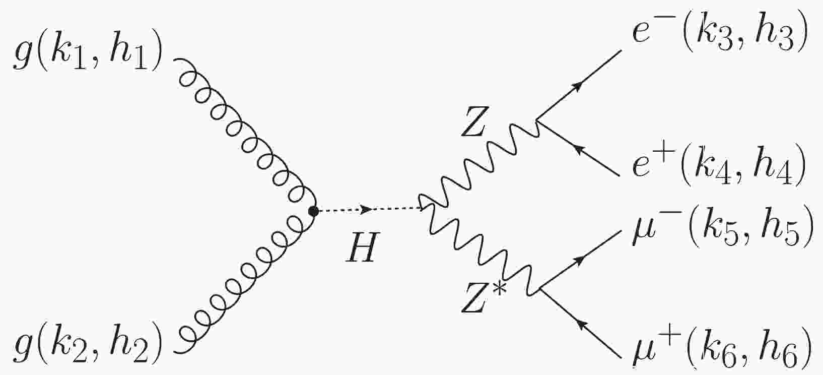
$ gg\to H\to ZZ\to2e2\mu $ in Fig. 1 is composed of three individual amplitudes$ A^H_{\rm{SM}}, A^H_{CP-{\rm{even}}} $ , and$ A^H_{CP-{\rm{odd}}} $ , which have the same production process but different Higgs decay modes according to the three kinds of$ HZZ $ vertices in Eq. (6). The specific formulas are
Figure 1. Feynman diagram of the Higgs-mediated process
$ gg \to H \to ZZ\to2e2\mu $ . The black dot represents an effective$ ggH $ coupling from loop contributions.${\cal{A}}^{gg\to H\to ZZ\to2e2\mu} (1_g^{h_1},2_g^{h_2},3_{e^-}^{h_3},4^{h_4}_{e^+},5_{\mu^-}^{h_5},6^{h_6}_{\mu^+}) $

(8) $ \begin{split}=& [a_1{\cal{A}}^{H}_{\rm{SM}}+a_2{\cal{A}}^{H}_{CP-{\rm{even}}}+a_3{\cal{A}}^{H}_{CP-{\rm{odd}}}]\\&\times (1_g^{h_1},2_g^{h_2},3_{e^-}^{h_3},4^{h_4}_{e^+},5_{\mu^-}^{h_5},6^{h_6}_{\mu^+})\; , \end{split}$

(9) $ \begin{split} =& {\cal{A}}^{gg\to H}(1_g^{h_1},2_g^{h_2})\times \frac{P_H(s_{12})}{s_{12}}\\&\times \sum\limits_{i = 1}^3 a_i{\cal{A}}_i^{H\to ZZ\to2e2\mu}(3_{e^-}^{h_3},4^{h_4}_{e^+},5_{\mu^-}^{h_5}, 6^{h_6}_{\mu^+})\; , \end{split} $

(10) where
$ h_i $ $ (i = 1\cdots 6) $ are helicity indices of external particles,$ s_{ij} = (k_i+k_j)^2 $ , and$ P_H(s) = \dfrac{s}{s-M_H^2+iM_H\Gamma_H} $ is the Higgs propagator.The production part
$ {\cal{A}}^{gg\to H}(1^{h_1}_g,2^{h_2}_g) $ is the helicity amplitude of gluon–gluon fusion to the Higgs process, in which$ h_1, h_2 $ represent the helicities of gluons with outgoing momenta. For all the other helicity amplitudes in this paper, we also keep the convention that the momentum of each external particle is outgoing. When writing the helicity amplitudes, we adopt the conventions used in [51,58]:$ \begin{split}& \langle ij \rangle = \bar{u}_-(p_i) u_+(p_j), \qquad \; \; {[ ij ]} = \bar{u}_+(p_i) u_-(p_j)\; ,\\& \langle ij \rangle[ ji ] = 2 p_i \cdot p_j, \qquad \; \; s_{ij} = (p_i+p_j)^2, \end{split} $

(11) and we have
$ \begin{split} &{\cal{A}}^{gg\to H}(1^{+}_g,2^{+}_g) = \frac{2c_g}{v}[12]^2\; , \\ & {\cal{A}}^{gg\to H}(1^{-}_g,2^{-}_g) = \frac{2c_g}{v}\langle12\rangle^2\; . \end{split} $

(12) To keep the
$ ggH $ coupling consistent with the SM, we use$ \frac{c_g}{v} = \frac{1}{2}\sum\limits_f\frac{\delta^{a b}}{2}\frac{\rm i}{16\pi^2}g^2_s4e \frac{m_f^2}{2M_W s_W}\frac{1}{s_{12}}[2+s_{12}(1-\tau_H)C^{\gamma\gamma}_0(m_f^2)]\; ,$

(13) with
$ C^{\gamma \gamma}_0(m^2) = 2\tau_H f(\tau_H)/4m^2\; , \tau_H = 4m^2/M^2_{H}, $

(14) $ f(\tau) = \left\{ \begin{array}{ll} {\rm{arcsin}}^2 \sqrt{1/\tau} & \tau \geqslant 1 \\ -\dfrac{1}{4} \left[ \log \dfrac{1 + \sqrt{1-\tau } } {1 - \sqrt{1-\tau} } - i \pi \right]^2 \ \ \ & \tau <1\; \end{array} \right.\; , $

(15) where
$ a, b = 1,...,8 $ are$ SU(3)_c $ adjoint representation indices for the gluons, the index$ f $ represents quark flavor, and$ C^{\gamma\gamma}_{0}(m^2) $ is the Passarino–Veltman three-point scalar function [59,60].The decay part
$ {\cal{A}}^{H\to ZZ\to2e2\mu}(3_{e^-}^{h_3},4^{h_4}_{e^+},5_{\mu^-}^{h_5},6^{h_6}_{\mu^+}) $ is the helicity amplitude of the process$ H\to ZZ\to e^-e^+\mu^-\mu^+ $ , which has three sources according to the three types of vertices as written in Eq. (6). Correspondingly, we write it as$ {\cal{A}}^{H\to ZZ\to2e2\mu}(3_{e^-}^{h_3},4^{h_4}_{e^+},5_{\mu^-}^{h_5},6^{h_6}_{\mu^+}) = \sum\limits_{i = 1}^3 a_i{\cal{A}}_i^{H\to ZZ\to2e2\mu}(3_{e^-}^{h_3},4^{h_4}_{e^+},5_{\mu^-}^{h_5},6^{h_6}_{\mu^+}) $

(16) with
$ {\cal{A}}_1^{H\to ZZ\to2e2\mu}(3^-_{e^-},4^+_{e^+},5^-_{\mu^-},6^+_{\mu^+}) = f \times l^2_e\frac{M_W^2}{\cos^2\theta_W}\langle35\rangle[46] , $

(17) $ {\cal{A}}_2^{H\to ZZ\to2e2\mu}(3^-_{e^-},4^+_{e^+},5^-_{\mu^-},6^+_{\mu^+}) = f\times l^2_e\times \Big[2k\cdot k^{\prime}\langle35\rangle[46] +\big(\langle35\rangle[45]+ \langle36\rangle[46]\big)\big(\langle35\rangle[36]+\langle45\rangle[46]\big) \Big], $

(18) $ \begin{split} {\cal{A}}_3^{H\to ZZ\to2e2\mu}(3^-_{e^-},4^+_{e^+},5^-_{\mu^-},6^+_{\mu^+}) =& f\times l^2_e\times (-i) \times \Big[2\big(k\cdot k^{\prime}+\langle46\rangle[46]\big)\langle35\rangle[46] +\langle35\rangle[45]\big(\langle35\rangle[36]+\langle45\rangle[46]\big) \\& +\langle36\rangle[46]\big(\langle35\rangle[36]-\langle45\rangle[46]\big)\Big]\; , \end{split} $

(19) and
$ f = -2{\rm i}e^3\frac{1}{M_W \sin\theta_W}\frac{P_Z(s_{34})}{s_{34}}\frac{P_Z(s_{56})}{s_{56}}\; , $

(20) where
$P_Z(s) = \dfrac{s}{s-M_Z^2+{\rm i}M_Z\Gamma_Z}$ is the$ Z $ boson propagator,$ M_Z $ ,$ M_W $ are the masses of the$ Z $ ,$ W $ bosons,$ \theta_W $ is the Weinberg angle, and$ l_e $ and$ r_e $ (will appear for other helicity combinations) are the coupling factors of the$ Z $ boson to left-handed and right-handed leptons:$ l_e = \frac{-1+2\sin^2\theta_W}{\sin(2\theta_W)}\, , \quad r_e = \frac{2\sin^2\theta_W}{\sin(2\theta_W)}\, . $

(21) In Eqs. (17)–(19), we only show the case in which the helicities of the four leptons (
$ h_3,h_4,h_5,h_6 $ ) are equal to ($ -,+,-,+ $ ). As for the other three non-zero helicity combinations ($ -,+,+,- $ ), ($ +,-,-,+ $ ), ($ +,-,+,- $ ), their helicity amplitudes are similar to Eqs. (17)–(19), but with some exchanges such as$ l_e \leftrightarrow r_e \; ,\; 4 \leftrightarrow 6\; ,\; 3 \leftrightarrow 5\; ,\; []\leftrightarrow \langle\rangle\; . $

(22) Their specific formulas are shown in Appendix A.
-
The box process
$ gg \to ZZ \to 2e2\mu $ is a continuum background of the Higgs-mediated$ gg\to H\to2e2\mu $ process. The interference between these two kinds of processes could have a nonnegligible contribution in the off-shell Higgs region. The Feynman diagram of the process$ gg \to ZZ \to 2e2\mu $ is a box diagram induced by fermion loops (see Fig. 2). The helicity amplitude$ A^{gg \to ZZ \to 2e2\mu}_{\rm{box}} $ has been calculated analytically and coded in the MCFM8.0 package. Another similar calculation using a different method can be found in gg2VV code [61].
Figure 2. Feynman diagram of the box process
$gg \to ZZ\to2e2\mu$ . -
The process
$ gg\to H\to ZZ \to 4\ell $ with identical$ 4e $ or$ 4\mu $ final states can also be used to probe the anomalous$ HZZ $ couplings. In the SM, the differential cross sections of the$ 4\ell $ (including both$ 4e $ and$ 4\mu $ ) and$ 2e2\mu $ processes are nearly the same in both the on-shell and off-shell Higgs regions [53], which indicates that adding the$ 4e/4\mu $ process could almost double experimental statistics. This situation is probably similar for the anomalous Higgs-mediated processes. The$ 4e/4\mu $ Feynman diagrams consist of two different topology structures as shown in Fig. 3. Figure 3(b) is different from Fig. 3(a) just as a result of swapping the positive charged leptons ($4 \leftrightarrow 6$ ). The helicity amplitude of each diagram is similar to the former$ 2e2\mu $ cases but needs to be multiplied by a symmetry factor 1/2. While calculating the total cross section, the interference term between Fig. 3(a) and (b) needs an extra factor of -1 compared to the self-conjugated terms because it connects all of the decayed leptons in one fermion loop, while each self-conjugated term has two fermion loops. After considering these details, the summed cross section of the$ 4e $ and$ 4\mu $ processes is comparable to the$ 2e2\mu $ process. More details are shown in the following numerical results.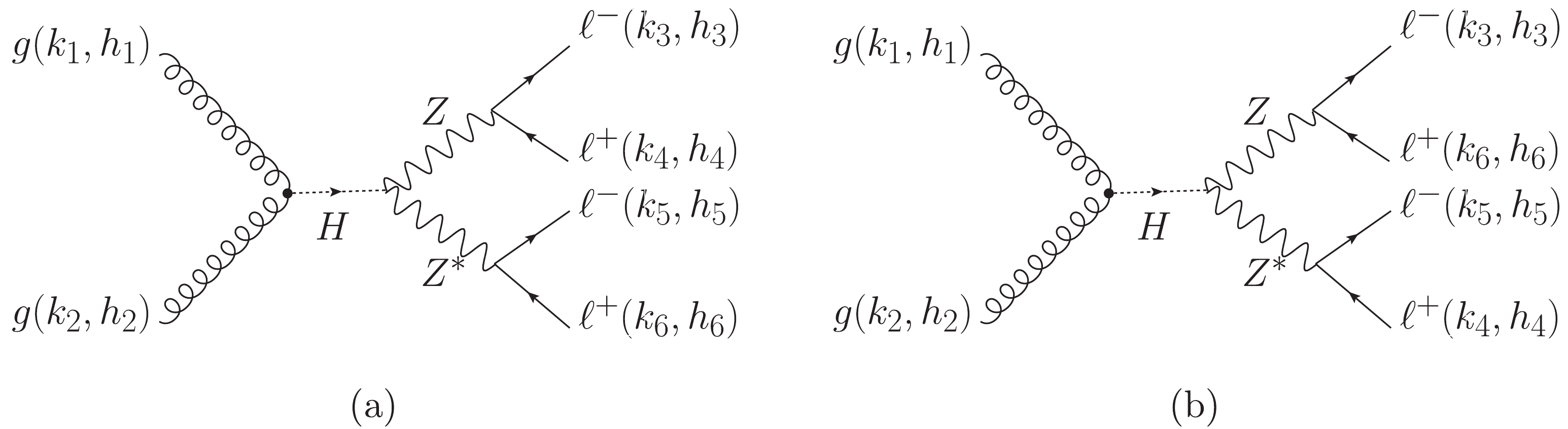
Figure 3. Feynman diagrams of the process
$ gg \to H\to ZZ\to 4\ell $ , where$ 4\ell = 4e\ {\rm{or}}\ 4\mu $ . Note that diagram (b) is obtained by swapping the two positive charged leptons ($4 \leftrightarrow 6$ ) in diagram (a). -
In this section we present the integrated cross sections and differential distributions in both the on-shell and off-shell Higgs regions, especially the interference between anomalous Higgs-mediated processes and SM processes.
-
To compare theoretical calculation with experimental observation at the LHC, we need to further calculate the cross sections at hadron level. From helicity amplitude to the cross section, two more steps are required. Firstly, we should sum and square the amplitudes to get the differential cross section at parton level, then integrate phase space and the parton distribution function (PDF) to get the cross section at hadron level. We show these two steps conceptually as follows.
The squared amplitude in the differential cross section at parton level
$ {\rm d}\hat{\sigma}(s_{12}) $ is$ \left|{\cal{A}}_{\rm{box}}^{gg\to ZZ\to 4\ell}+{\cal{A}}^{gg\to H \to ZZ\to 4\ell}\right|^2 $

(23) $ \begin{split} =& \bigg|{\cal{A}}_{\rm{box}}^{gg\to ZZ\to 4\ell}+{\cal{A}}^{H}_{\rm{SM}}+ a_1{\cal{A}}^{H}_{\rm{SM}}+a_2{\cal{A}}^{H}_{CP-{\rm{even}}}\\&+a_3{\cal{A}}^{H}_{CP-{\rm{odd}}} \bigg|^2\; . \end{split}$

(24) After expanding it, there remain self-conjugated terms and interference terms that have different amplitude sources. As in the next step the integral of phase space and the PDF are the same for each term, we note the integrated cross sections separately by the amplitude sources, which are
$ \sigma_{k,l}\sim \left\{ \begin{array}{ll} |{\cal{A}}_k|^2, \quad\quad & k = l ;\\ 2{\rm{Re}}({\cal{A}}^\ast_k{\cal{A}}_l), \quad\quad& k\ne l ,\\ \end{array} \right. $

(25) where
$ k,l$ = {box, SM, CP-even, CP-odd}. The superscripts of$ {\cal{A}} $ are omitted for brevity. -
We form the integral of phase space and the PDF in the MCFM 8.0 package [62,63]. The simulation is performed for the proton–proton collision at the center-of-mass energy
$ \sqrt{s} = 13 $ TeV. The Higgs mass is set to be$ M_H = 125 \; {\rm{GeV}} $ . The renormalization$ \mu_r $ and factorization scale$ \mu_f $ are set as the dynamic scale$ m_{4\ell}/2 $ . For the PDF we choose the leading-order MSTW 2008 PDFs MSTW08LO [64]. Some basic phase space cuts are exerted as follows, which are similar to the event selection cuts used in the CMS experiment [65].$ \begin{split}& P_{T,\mu}>5{\rm{GeV}}, \ |\eta_{\mu}|<2.4\; ,\;\; P_{T,e}>7{\rm{GeV}}, \ |\eta_{e}|<2.5\; ,\\& \ m_{\ell\ell}>4 {\rm{GeV}}, \ m_{4\ell}>100{\rm{GeV}}\; . \end{split} $

(26) Besides, for the
$ 2e2\mu $ channel, the hardest (second-hardest) lepton should satisfy$ P_T> 20\; (10){\rm{GeV}} $ ; one pair of leptons with the same flavour and opposite charge is required to have$ 40 {\rm{GeV}}<m_{\ell^+\ell^-}<120 {\rm{GeV}} $ and the other pair needs to fulfill$ 12 {\rm{GeV}} <m_{\ell^+\ell^-}<120 {\rm{GeV}} $ . For the$ 4e $ or$ 4\mu $ channel, four oppositely charged lepton pairs exist as$ Z $ boson candidates. The selection strategy is to first choose one pair nearest to the$ Z $ boson mass as one$ Z $ boson, then consider the left two leptons as the other$ Z $ boson. The other requirements are similar to those of the$ 2e2\mu $ channel.Table 1 shows the cross sections
$ \sigma_{k,l} $ with$ k,l$ = {box, SM,$ CP $ -even,$ CP $ -odd}, while$ a_1,a_2,a_3 $ are all set to 1 for convenience. The cross-section values can be converted easily by multiplying a scale factor for small$ a_i $ s. In the left and right panels, the integral regions of$ m_{4\ell} $ are set as$ m_{4\ell}<130\; {\rm{GeV}} $ and$ m_{4\ell}>220\; {\rm{GeV}} $ , which correspond to the on-shell and off-shell Higgs regions, respectively. Next, we focus on two kinds of interference effects: the interference between each Higgs-mediated process and the box continuum background, denoted as$ \sigma_{{\rm{box}},l} $ (or$ \sigma_{l,{\rm{box}}} $ ) with$ l\ne{\rm{box}} $ ; and the interference between different Higgs-mediated processes, denoted as$ \sigma_{k,l} $ with$ k,l\ne {\rm{box}} $ .13 TeV, $m_{2e2\mu} < 130\;{\rm {GeV} }$ , on-shell

13 TeV, $m_{2e2\mu}>220\;{\rm{GeV}}$ , off-shell

$\sigma_{k,l}$ /fb

box Higgs-med. $\sigma_{k,l}$ /fb

box Higgs-med. SM CP-even CP-odd SM CP-even CP-odd box 0.024 0 0 0 box 1.283 −0.174 −0.571 0 Higgs-med. SM 0 0.503 0.558 0 Higgs-med. SM −0.174 0.100 0.137 0 CP-even 0 0.558 0.202 0 CP-even −0.571 0.137 0.720 0 CP-odd 0 0 0 0.075 CP-odd 0 0 0 0.716 Table 1. Cross sections of
$ gg\to2e2\mu $ processes in proton–proton collisions at center-of-mass energy$ \sqrt{s} = 13 $ TeV with$ a_1 = 0, a_2 = a_3 = 1 $ in Eq. (6).The interference terms between Higgs-mediated processes and the continuum background
$ \sigma_{{\rm{box}},l} $ are all zero in the on-shell Higgs region, but relatively sizeable in the off-shell regions except for the cases with the$ CP $ -odd Higgs-mediated process, as shown in Table 1. There is an interesting reason for this. From Eqs. (9), (10), and (25),$ \begin{split} \sigma_{{\rm{box}},l} \sim & 2{\rm{Re}}({\cal{A}}^\ast_{\rm{box}}{\cal{A}}_l)\; ,\\ \sim & 2{\rm{Re}}\big({\cal{A}}^\ast_{\rm{box}} {\cal{A}}^{gg\to H}P_H(s_{12}){\cal{A}}_i\big)\; ,\\ \sim & 2\frac{(s_{12}-M^2_H){\rm{Re}}\big({\cal{A}}^\ast_{\rm{box}}{\cal{A}}^{gg\to H}{\cal{A}}_i\big)+M_H\Gamma_H{\rm{Im}}\big({\cal{A}}^\ast_{\rm{box}}{\cal{A}}^{gg\to H}{\cal{A}}_i\big)} {(s_{12}-M^2_H)^2+M^2_H\Gamma^2_H}\; , \end{split} $

(27) which means the integrand of
$ \sigma_{{\rm{box}},l} $ consists of two parts: one is antisymmetric around$ M^2_H $ , and the other is proportional to$ M_H\Gamma_H{\rm{Im}}\big({\cal{A}}^\ast_{\rm{box}}{\cal{A}}^{gg\to H}{\cal{A}}_i\big) $ . The first part can be largely suppressed almost to zero in the integral with a symmetric integral region around$ M_H $ . The second part is also suppressed not only by the small factor of$ \Gamma_H/M_H $ but also by a small value of$ {\rm{Im}}\big({\cal{A}}^\ast_{\rm{box}}{\cal{A}}^{gg\to H}{\cal{A}}_i\big) $ in the on-shell Higgs region. By contrast, in the off-shell Higgs region the integral regions are not symmetric around$ M_H $ but larger on one side than$ M_H $ , which means the first term has a nonzero contribution. Both the first and second terms can also be enhanced when$ \sqrt{s_{12}} $ is a little larger than twice the top quark mass. This is because the$ gg\to H $ process is induced mainly by the top quark loop; both the real part and the imaginary part of the amplitude (Re$ {\cal{A}}^{gg\to H} $ and Im$ {\cal{A}}^{gg\to H} $ ) can be enhanced when$ \sqrt{s_{12}} $ is just larger than the$ 2M_t $ threshold (see Eq. (13)). Thus,$ {\rm{Im}}\big({\cal{A}}^\ast_{\rm{box}}{\cal{A}}^{gg\to H}{\cal{A}}_i\big) $ can have a larger value, even though the relative contribution from the second term can be still suppressed by the smallness of the factor$ \Gamma_H/M_H $ . In conclusion, mainly due to the nonsymmetric integral region and some enhancement of$ {\cal{A}}^{gg\to H} $ , the interference contribution in the off-shell Higgs region becomes comparable with the self-conjugated contributions.It is also worthwhile to point out that there is no cross-section contribution from the interference between the
$ CP $ -odd Higgs-mediated process and other three processes, which include the continuum background process, SM Higgs-mediated process and anomalous$ CP $ -even Higgs-mediated process. This is because there is an antisymmetric tensor$ \epsilon^{\mu\nu\rho\sigma} $ in the$ CP $ -odd$ HZZ $ interaction vertex (see last term in Eq. (6)), while in the other three processes, the two indices are symmetrically paired and so the contrast of the indices makes the interference term zero. Nevertheless, these$ CP $ -odd interference term can show angular distributions, including the polar angle distribution of$ \ell $ in the$ Z $ boson rest frame and the azimuthal angular distribution between two$ z $ decay planes [33,36], even though its contribution to the total cross section is still zero.The interference between the
$ CP $ -even Higgs-mediated process and SM Higgs-mediated process is nonnegligible both in the on-shell and off-shell Higgs regions. In the on-shell Higgs region, the contribution from the interference terms is larger than that from the self-conjugated terms. Furthermore, for the$ a_1 = 0, a_2 = -1 $ choice (as in [10]), the interference terms have a minus sign, compared to the relative values in Table 1, which makes the total contribution of the$ CP $ -even Higgs-mediated process beyond the SM a destructive effect. In the off-shell region, the$ CP $ s-even Higgs-mediated process has two interference terms, between both the SM Higgs-mediated process and the box process. These two interference terms have opposite signs, which means they partly cancel each other out. However, the summed interference effect is still comparable to the self-conjugated contribution.Figure 4 shows the differential cross sections. The black histogram is from its main background process
$ q\bar{q}\to 2e 2\mu $ , which is a high background but still controllable. The red dashed histogram is from the SM$ gg\to 2e 2\mu $ processes including contributions from both the box and SM Higgs-mediated amplitudes. The blue dotted histogram adds contribution from the$ CP $ -even Higgs mediated amplitude to the SM signal and background amplitudes. Therefore, three kinds of interference terms are included. For comparison, we also show the green dashed-dotted histogram without interference terms from the$ CP $ -even Higgs amplitudes with others, so the interference contribution can be calculated by the difference between the blue and green histograms. In the on-shell region we can see the$ CP $ -even Higgs-mediated process has a total positive contribution (blue histogram) compared to the SM process (red histogram), while the green histogram shows the main positive contribution is from the interference term. In the off-shell region, the interference contribution is obvious in the$ 200\; {\rm{GeV}} < m_{4\ell} < 600\; {\rm{GeV}} $ region. There is a bump in the blue and green histograms when$ m_{4\ell}\approx350 $ GeV, which is caused by the total cross section of the$ CP $ -even Higgs-mediated process increasing suddenly beyond the$ 2M_t $ (twice the top quark mass) threshold. The differential cross section for the$ CP $ -odd Higgs-mediated process is similar to the green histogram in the off-shell region as it has no interference contribution after the angular distributions are integrated.
Figure 4. (color online) Differential cross sections of the
$ gg\to2e2\mu $ processes and$ q\bar{q}\to2e2\mu $ process in proton–proton collision at$ \sqrt{s} = 13 $ TeV with$ a_2 = 1, a_1 = a_3 = 0 $ in Eq. (6).The numerical results at center-of-mass energy
$ \sqrt{s} = 8 $ TeV are shown in Table B1 in Appendix B. By comparing them to the results at$ \sqrt{s} = 13 $ TeV in Table 1, we find that each cross section is decreased by about one or two times and their relative ratios have some minor changes. This could be caused by both PDF functions and kinematic distributions.8 TeV, $m_{2e2\mu} < 130{\rm{GeV}}$ , on-shell

8 TeV, $m_{2e2\mu}>220{\rm{GeV}}$ , off-shell

$\sigma_{k,l}$ /fb

box Higgs-med. $\sigma_{k,l}$ /fb

box Higgs-med. SM CP-even CP-odd SM CP-even CP-odd box 0.011 0 0 0 box 0.479 −0.056 −0.198 0 Higgs-med. SM 0 0.232 0.257 0 Higgs-med. SM −0.056 0.031 0.047 0 CP-even 0 0.257 0.093 0 CP-even −0.198 0.047 0.228 0 CP-odd 0 0 0 0.035 CP-odd 0 0 0 0.219 Table B1. Cross sections of
$ gg\to2e2\mu $ processes in proton–proton collisions at$ \sqrt{s} = 8 $ TeV with$ a_1 = 0,a_2 = a_3 = 1 $ in Eq. (6). -
The cross sections of the
$ gg\to4e/4\mu $ processes are listed in Table 2 (Table B2 in Appendix B) for comparison and future use. Here,$ gg\to4e/4\mu $ represents the sum of$ gg\to4e $ and$ gg\to 4\mu $ . Comparing Table 2 with Table 1, the numbers in the right panels are similar, while the numbers in the left panels have relatively large differences. This is mainly because of the different selection cuts [53]. If we apply the$ 4e/4\mu $ selection cuts to the$ gg\to 2e2\mu $ process,$ \sigma_{\rm{box, box}} $ in the left panels become similar.13 TeV, $m_{4e/4\mu} < 130\;{\rm{GeV}}$ , on-shell

13 TeV, $m_{4e/4\mu}>220\;{\rm{GeV}}$ , off-shell

$\sigma_{k,l}$ /fb

box Higgs-med. $\sigma_{k,l}$ /fb

box Higgs-med. SM CP-even CP-odd SM CP-even CP-odd box 0.045 0 0 0 box 1.303 −0.176 −0.575 0 Higgs-med. SM 0 0.540 0.568 0 Higgs-med. SM −0.176 0.101 0.137 0 CP-even 0 0.568 0.186 0 CP-even −0.575 0.137 0.740 0 CP-odd 0 0 0 0.060 CP-odd 0 0 0 0.708 Table 2. Cross sections of
$ gg\to4e/4\mu $ processes in proton–proton collisions at center-of-mass energy$ \sqrt{s} = 13 $ TeV with$ a_1 = 0, a_2 = a_3 = 1 $ in Eq. (6).8 TeV, $m_{4e/4\mu} < 130{\rm{GeV}}$ , on-shell

8 TeV, $m_{4e/4\mu}>220{\rm{GeV}}$ , off-shell

$\sigma_{k,l}$ /fb

box Higgs-med. $\sigma_{k,l}$ /fb

box Higgs-med. SM CP-even CP-odd SM CP-even CP-odd box 0.021 0 0 0 box 0.485 −0.056 −0.199 0 Higgs-med. SM 0 0.248 0.261 0 Higgs-med. SM −0.056 0.031 0.047 0 CP-even 0 0.261 0.086 0 CP-even −0.199 0.047 0.229 0 CP-odd 0 0 0 0.028 CP-odd 0 0 0 0.215 Table B2. Cross sections of
$ gg\to4e/4\mu $ processes in proton–proton collisions at center-of-mass energy$ \sqrt{s} = 8 $ TeV with$ a_1 = 0, a_2 = a_3 = 1 $ in Eq. (6). -
In this section we show a naive estimation to constrain
$ a_1 $ ,$ a_2 $ and$ a_3 $ by using the data in both the on-shell and off-shell Higgs regions.First, we estimate the expected number of events
$ N^{\exp}(a_1, a_2,a_3) $ in the off-shell Higgs region, which is defined as the contribution from the processes with anomalous couplings after excluding the pure SM contributions.A theoretical observed total number of events should be
$ N^{\rm{theo}}(a_1,a_2,a_3) = \sigma_{\rm{tot}}\times {\cal{L}}\times k\times\epsilon\; , $

(28) where
$ \sigma_{\rm{tot}} $ is the total cross section,$ {\cal{L}} $ is the integrated luminosity,$ k $ represents the$ k $ -factor and$ \epsilon $ is the total efficiency.The simulation in the CMS experiment [47] with an integrated luminosity of
$ {\cal{L}}\sim 80 $ fb$ ^{-1} $ at$ \sqrt{s} = 13 $ TeV shows that for the$ gg\to4\ell $ process, the expected numbers of events in the off-shell Higgs region ($ m_{4\ell}>220{\rm{GeV}} $ ) can be divided into two categories:$ N_{gg\; \; {\rm{signal}}} = 20.3 $ and$ N_{gg\; \; {\rm{interference}}} = -34.4 $ , where the subscript "$ gg $ signal" represents the SM Higgs-mediated signal term, and "$ gg $ interference" represents the interference term between the SM Higgs-mediated process and the box process. For high-order corrections that may change the$ k $ -factor, some existing studies [66-69] show that the loop corrections on the box diagram (Fig. 2) and the Higgs-mediated diagram are different. Therefore, we also group the expected event numbers contributed from the anomalous couplings into two categories.$ \begin{split} N^{\exp}(a_1,a_2,a_3) \!=\! & \frac{N_{gg\; \; {\rm{signal}}}}{\sigma^{H}_{\rm{SM}}} \!\times\![(a_1\!+\!1)^2\sigma_{\rm{SM}}^H\!-\!\sigma_{\rm{SM}}^H\!+\!a^2_2\sigma^H_{CP-{{\rm{even}}}} \\&+a^2_3\sigma^H_{CP-{\rm{odd}}}+(a_1+1)a_2\sigma_{CP-{{\rm{even}}},{\rm{SM}}}^{\rm{int}}]\\& + \frac{N_{gg\; \; {\rm{interference}}}}{\sigma^{\rm{int}}_{\rm{SM}}} \times[a_1\sigma_{{\rm{SM}},{\rm{box}}}^{\rm{int}}\\&+a_2\sigma^{\rm{int}}_{CP-{{\rm{even}},{\rm{box}}}}],\\[-15pt] \end{split} $

(29) where
$ N^{\exp}(a_1,a_2,a_3) $ represents the expected number of events from anomalous$ CP $ -even and$ CP $ -odd processes,$ \sigma_k^H $ is the self-conjugated Higgs-mediated cross section, and$ \sigma_{k,l}^{\rm{int}} $ is the interference cross section with$ k,l$ = {box, SM,$ CP $ -even,$ CP $ -odd}. The first term on the right-hand side of the equation is the contribution from the s-channel processes, and the second part is the contribution from the interference between the s-channel processes and the box diagram. For each category with the same topological Feynman diagrams, it is assumed to have the same$ k $ -factor and total efficiency$ \epsilon $ , which are equal to the corresponding values for the SM process. These coefficients are extracted from experimental measurements, which are similar to the treatment in the experiments [47,53].The cross section of the
$ 4\ell $ final states is the sum of the cross sections of the$ 2e2\mu $ ,$ 4e $ and$ 4\mu $ final states.$ N^{\exp}(a_1,a_2,a_3) $ can be obtained by combining the corresponding cross sections from both Table 1 and Table 2.The experimental observed number
$ N^{\rm{obs}}(a_1,a_2,a_3) $ that corresponds to$ N^{\exp}(a_1,a_2,a_3) $ is defined as$ N^{\rm{obs}}(a_1,a_2,a_3) = N_{\rm{total\; \; observed }}-N^{\rm{SM}}_{\rm{total\; \; expected} } = 38.7 $ in the CMS experiment [47]. Its fluctuation is estimated as the$ \delta_{\rm{off-shell}} = \sqrt{N_{\rm{total\; \;observed}}} = \sqrt{1325} $ (including both signal and background).Second, the observed signal strength of the
$ gg\to H\to 4l $ process measured by CMS [70] is$ \mu_{ggH}^{\rm{obs}} = 0.97^{+0.09}_{-0.09}{\rm{(stat.)}}^{+0.09}_{-0.07}{\rm{(syst.)}} $ . Its fluctuation is$ \delta_{\rm{on-shell}} = 0.127$ after a combination of both statistical and systematic errors. Theoretically, the signal strength with anomalous couplings can be estimated as$\begin{split}\mu_{ggH}^{\rm{exp}}(a_1,a_2,a_3) =& \frac{1}{\sigma_{\rm{SM}}^H}[(a_1+1)^2\sigma_{\rm{SM}}^H+a_2^2\sigma_{CP-{\rm{even}}}^H\\&+a_3^2\sigma_{CP-{\rm{odd}}}^H+(a_1+1)a_2\sigma_{CP-{\rm{even}},{\rm{SM}}}^{\rm{int}}], \end{split}$

(30) where
$ \sigma_k^H $ and$ \sigma_{k,l}^{\rm{int}} $ are same as in Eq. (29) except in the on-shell region. Equation (30) is shorter than Eq. (29) because in the on-shell Higgs region the interference term with box diagram$ \sigma_{\rm{SM, box}} $ and$ \sigma_{CP-\rm{even, box}} $ are zero.The survival parameter regions of
$ a_1,a_2 $ and$ a_3 $ can be obtained by a global$ \chi^2 $ fit, which can be constructed as$ \chi^2 = \left(\frac{N^{\exp}-N^{\rm{obs}}}{\delta_{\rm{off-shell}}}\right)^2+\left(\frac{\mu_{ggH}^{\exp}-\mu_{ggH}^{\rm{obs}}}{\delta_{\rm{on-shell}}}\right)^2. $

(31) The adoption of the
$ \chi^2 $ fit here can be controversial, as we only have two input data points (on-shell and off-shell) and have to find parameter regions for three variables ($ a_1,a_2 $ , and$ a_3 $ ). We claim that the result here is just for a complete analysis including both theoretical calculation and experimental constraints, and it is very preliminary. The situation can be improved if experimental collaborations can collect sufficient statistics in the future. Nevertheless, the$ \chi^2 $ fit can also provide some interesting results.Figure 5 shows the two-dimensional contour diagram of the anomalous couplings. There are three colored regions (green, blue, and red) in each small plot and the red areas are the final
$ 1\sigma $ survival parameter regions from the global$ \chi^2 $ fit. In the actual two-dimensional fitting procedure, we take two anomalous couplings to be free and fix the third one to be zero. Three individual$ \chi^2 $ fits are operated: constraint only from the off-region (first part in Eq. (31)), constraint from the on-shell region (second part in Eq. (31)), and a combination of the two. The purpose is to show how the irregular overlapping red regions emerge. As discussed in the above sections, we have an equal number of experimental data points and free parameters here and the$ \chi^2 $ fit degenerates to an equation-solving problem. Survival parameter regions from either the on-shell or off-shell constraint come to be concentric circles and the global fitting results are almost the overlap region between them.
Figure 5. (color online) Two-dimensional constraints on the new physics coefficients
$ a_1 $ ,$ a_2 $ and$ a_3 $ from$ \chi^2 $ fits. To illustrate the constraints from different energy regions, three$ 1\sigma $ regions (green concentric circles, blue concentric circles, and red region) from three individual$ \chi^2 $ fits (on-shell, off-shell, and both, respectively) are drawn here. CMS$ 2\sigma $ constraints (95% confidence level) [47] are drawn as the lines (magenta for$ a_2 $ when$ a_1 = a_3 = 0 $ and grey for$ a_3 $ when$ a_1 = a_2 = 0 $ ) in the right zoomed-in plots.The recently updated CMS experiment [47] uses both on-shell and off-shell data, constructs kinematic discriminants, and gets the limit (at 95% confidence level) of the parameters
$ a_2\subset [-0.09,0.19] $ ,$ a_3\subset [-0.21,0.18] $ (there is no corresponding constraint on$ a_1 $ ). This experimental analysis is based on one free parameter-fitting schedule so we draw them as the line segments in the right plots of Fig. 5 (magenta for$ a_2 $ and grey for$ a_3 $ ). Our global fit results are roughly consistent with those of the CMS, although at first glance the two appear to have some conflict (note that we draw a$ 1\sigma $ contour, whereas the CMS results are the limit at 95% confidence level, which corresponds to$ 2\sigma $ intervals in the hypothesis of Gaussian distribution). The CMS results seem to be more stringent than ours. This may be caused by their use of more detailed kinematic information in their analysis. Besides, we have some parameter regions with$ a_1\sim -2 $ or$ a_2 $ approaching 1. These regions show the correlation of each pair of parameters. There is cancellation on the cross sections when the parameters coexist. In principle, the anomalous couplings should be much smaller than 1 to validate the operator expansion. Therefore, these parameter regions should be ruled out. Nonetheless, our global fit provides a complementary perspective of how the final anomalous coupling parameters contour regions are obtained from the individual on-shell/off-shell energy region constraints. These preliminary fitting results can be optimized in the case of more statistics in the future. -
When considering the anomalous
$ HZZ $ couplings, we calculate the cross sections induced by these new couplings, and special attention is focused on the interference effects. In principle, there are three kinds of interference: 1. the interference between the anomalous$ CP $ -even Higgs-mediated process and the continuum background box process$ \sigma_{CP{\rm{-even}},{\rm{box}}} $ ; 2. the interference between the anomalous$ CP $ -even Higgs-mediated process and the SM Higgs-mediated process$ \sigma_{CP{\rm{-even}},{\rm{SM}}} $ ; and 3. the interference between the anomalous$ CP $ -odd Higgs-mediated process and all other processes$ \sigma_{CP{\rm{-odd}},k} $ with$ k = {{\rm{box}}, {\rm{SM}}, CP{\rm{-even}}} $ . The numerical results of the integrated cross sections show that the first kind of interference can be neglected in the on-shell Higgs region but is nonnegligible in the off-shell Higgs region, the second kind of interference is important in both the on-shell and off-shell Higgs regions, and the third kind of interference has zero contribution for the total cross section in both regions.By using the theoretical calculation together with both on-shell and off-shell Higgs experimental data, we estimate the constraints on the anomalous
$ HZZ $ couplings. The correlations of the different kinds of anomalous couplings are shown in contour plots, which illustrate how the anomalous contributions cancel each other out and the extra parameter regions survive when they coexist.In this research we only use the numerical results of integrated cross sections, whereas in fact more information could be fetched from the differential cross sections (kinematic distributions). Furthermore, the
$ k $ -factors and total efficiencies should also be estimated separately according to different sources. We leave them for our future work.We thank John M. Campbell for his helpful explanation of the code in the MCFM package.
-
The helicity amplitudes
$ {\cal{A}}_1 $ ,$ {\cal{A}}_2 $ , and$ {\cal{A}}_3 $ are shown separately. The common factor$ f $ is defined as$ f = -2ie^3\frac{1}{M_W \sin\theta_W}\frac{P_Z(s_{34})}{s_{34}}\frac{P_Z(s_{56})}{s_{56}}\; . $

$ \begin{aligned}[b] & {\cal{A}}_1^{H\to ZZ\to2e2\mu}(3^-_{e^-},4^+_{e^+},5^-_{\mu^-},6^+_{\mu^+}) = f \times l^2_e\frac{M_W^2}{\cos^2\theta_W}\langle35\rangle[46] , \quad {\cal{A}}_1^{H\to ZZ\to2e2\mu}(3^-_{e^-},4^+_{e^+},5^+_{\mu^-},6^-_{\mu^+}) = f \times l_er_e\frac{M_W^2}{\cos^2\theta_W}\langle36\rangle[45] , \\& {\cal{A}}_1^{H\to ZZ\to2e2\mu}(3^+_{e^-},4^-_{e^+},5^-_{\mu^-},6^+_{\mu^+}) = f \times l_er_e\frac{M_W^2}{\cos^2\theta_W}\langle45\rangle[36] , \quad {\cal{A}}_1^{H\to ZZ\to2e2\mu}(3^+_{e^-},4^-_{e^+},5^+_{\mu^-},6^-_{\mu^+}) = f \times r^2_e\frac{M_W^2}{\cos^2\theta_W}\langle46\rangle[35] \; . \end{aligned}\tag{{A1}\normalsize}$

$ \begin{split} &{\cal{A}}_2^{H\to ZZ\to2e2\mu}(3^-_{e^-},4^+_{e^+},5^-_{\mu^-},6^+_{\mu^+}) = f\times l^2_e\times \Big[2k\cdot k^{\prime}\langle35\rangle[46] +\big(\langle35\rangle[45]+ \langle36\rangle[46]\big)\big(\langle35\rangle[36]+\langle45\rangle[46]\big) \Big], \\& {\cal{A}}_2^{H\to ZZ\to2e2\mu}(3^-_{e^-},4^+_{e^+},5^+_{\mu^-},6^-_{\mu^+}) = f\times l_er_e\times \Big[2k\cdot k^{\prime}\langle36\rangle[45] +\big(\langle35\rangle[45]+ \langle36\rangle[46]\big)\big(\langle36\rangle[35]+\langle46\rangle[45]\big) \Big], \\& {\cal{A}}_2^{H\to ZZ\to2e2\mu}(3^+_{e^-},4^-_{e^+},5^-_{\mu^-},6^+_{\mu^+}) = f\times r_el_e\times \Big[2k\cdot k^{\prime}\langle45\rangle[36] +\big(\langle45\rangle[35]+ \langle46\rangle[36]\big)\big(\langle35\rangle[36]+\langle45\rangle[46]\big) \Big], \\ & {\cal{A}}_2^{H\to ZZ\to2e2\mu}(3^+_{e^-},4^-_{e^+},5^+_{\mu^-},6^-_{\mu^+}) = f\times r^2_e\times \Big[2k\cdot k^{\prime}\langle46\rangle[35] +\big(\langle45\rangle[35]+ \langle46\rangle[36]\big)\big(\langle36\rangle[35]+\langle46\rangle[45]\big) \Big]. \end{split} \tag{{A2}\normalsize}$

(A2) $ \begin{split}\quad\quad\quad {\cal{A}}_3^{H\to ZZ\to2e2\mu}(3^-_{e^-},4^+_{e^+},5^-_{\mu^-},6^+_{\mu^+}) =& f\times l^2_e\times (-i) \times \Big[2\big(k\cdot k^{\prime}+\langle46\rangle[46]\big)\langle35\rangle[46] +\langle35\rangle[45]\big(\langle35\rangle[36]+\langle45\rangle[46]\big) \\& +\langle36\rangle[46]\big(\langle35\rangle[36]-\langle45\rangle[46]\big)\Big]\; , \\ {\cal{A}}_3^{H\to ZZ\to2e2\mu}(3^-_{e^-},4^+_{e^+},5^+_{\mu^-},6^-_{\mu^+}) =& f\times l_er_e\times (-i) \times \Big[2\big(k\cdot k^{\prime}+\langle45\rangle[45]\big)\langle36\rangle[45] +\langle36\rangle[46]\big(\langle36\rangle[35]+\langle46\rangle[45]\big) \\& +\langle35\rangle[45]\big(\langle36\rangle[35]-\langle46\rangle[45]\big)\Big], \\ {\cal{A}}_3^{H\to ZZ\to2e2\mu}(3^+_{e^-},4^-_{e^+},5^-_{\mu^-},6^+_{\mu^+}) =& f\times r_el_e\times (-i) \times \Big[2\big(k\cdot k^{\prime}+\langle36\rangle[36]\big)\langle45\rangle[36] +\langle45\rangle[35]\big(\langle45\rangle[46]+\langle35\rangle[36]\big) \\& +\langle46\rangle[36]\big(\langle45\rangle[46]-\langle35\rangle[36]\big)\Big], \\ {\cal{A}}_3^{H\to ZZ\to2e2\mu}(3^+_{e^-},4^-_{e^+},5^+_{\mu^-},6^-_{\mu^+}) =& f\times r^2_e\times (-i) \times \Big[2\big(k\cdot k^{\prime}+\langle35\rangle[35]\big)\langle46\rangle[35] +\langle46\rangle[36]\big(\langle46\rangle[45]+\langle36\rangle[35]\big) \\& +\langle45\rangle[35]\big(\langle46\rangle[45]-\langle36\rangle[35]\big)\Big]. \end{split} \tag{{A3}\normalsize}$

(34)
Anomalous ${{H\to ZZ \to 4\ell}}$ decay and its interference effects on gluon–gluon contribution at the LHC
- Received Date: 2020-01-12
- Accepted Date: 2020-07-08
- Available Online: 2020-12-01
Abstract: We calculate the spinor helicity amplitudes of anomalous


 DownLoad: