


 Abstract
 HTML
HTML Reference
 Related
 PDF
PDF


-
After the discovery of the accelerated expansion of the universe [1, 2], several hypotheses have been proposed to address the dark energy problem, such as Horndeski theories [3-5], generalized proca theories [6, 7], and the ghost-free massive gravity [8, 9]. However, the discovery of gravitational waves GW170817 [10] severely constrains these modified gravity models [11-13]. The simplest standard model of cosmology, without the introduction of any new gravitational degrees of freedom, is the
$ \Lambda $ CDM. Based on the proposal of “minimal” dark matter and dark energy components, it could reasonably explain the accelerated expansion of the universe, as well as other observational data, until recently [14]. A number of low-redshift observations have revealed that there are discrepancies between the values of the Hubble parameter at the present time,$ H_{0} $ , based on observations of Cepheids in the Large Magellanic Cloud (LMC) [15], the gravitational lensing of quasar measurements [16, 17], and the predicted value obtained from the Planck CMB data within the$ \Lambda $ CDM (Note that an intermediate value was originally found using Red Giants as the distance ladder [18]. These values were subsequently corrected to a value consistent with the low-redshift measurements [19]). Since the difference between$ H_0 $ is approximately$ 5 \sigma $ , this means that the standard model of cosmology, the$ \Lambda $ CDM, may not be correct. There is a tension between the$ H_{0} $ predicted from the early universe and the values obtained by direct measurements at low redshifts.Many ideas have been proposed to resolve the Hubble tension, such as the modified gravity and brane model [20-23], the gravitational and vacuum [24-26] phase transition, early dark energy [27], dark matter decay [28], dark sector interaction [29, 30], neutrino self-interaction [31], phenomenological dark energy [32], and the negative cosmological constant [33] (moreover, see [34]). In this work, we demonstrate that the usual Friedmann equation allows for a higher value of
$ H_{0} = 74.03\; \rm{km\; s}^{-1}\rm{Mpc}^{-1} $ while keeping the matter contribution to 31% and the dark energy contribution to 69%, provided that an extra component with a very small negative density is introduced. The negative component must be a very small fraction to the total density of the universe; otherwise, it would have been previously detected (see Ref. [35], except for the possible galactic effects of a small negative density on the rotation curves). As a theoretical model that considers such a possibility, we propose a modified quintom model [36] to realize the negative-density component that is phenomenologically required by the Friedmann equation. The quintom model consists of a quintessence scalar field and a phantom scalar field. The model introduces dark energy with phantom divide crossing and a stable late-time solution. The use of two scalar fields for dark energy is not novel (see e.g. [37-39]. It is shown in Ref. [40] that a model with only one quintessence scalar and a cosmological constant exacerbates the Hubble tension. A model called the gravitational scalar-tensor theory also incudes two scalar fields [41, 42]. It is interesting to examine whether the phantom scalar field of the quintom model matches the required negative density and is capable of addressing the Hubble tension.This work is organized as follows. Section II discusses the physical requirement of the extra component X for coexistence within the standard Friedmann model to alleviate the Hubble tension. In Section III, we propose a modified quintom model with scalar-matter coupling that realizes the negative density requirement, giving the correct value of
$ H_{0} $ while keeping the density parameters$ \Omega_{m}^{(0)}\simeq 0.31, \Omega_{\rm DE}^{(0)}\simeq 0.69 $ consistent with Planck's early universe constraints. We use a dynamical system approach to find cosmological solutions of the modified quintom model in Section IV. Section V presents the numerical analysis results of the quintom model, yielding a realistic cosmological solution. Section VI compares the theoretical prediction of our model to the observational data, and Section VII summarizes our main results. -
In this section, a general physical condition is discussed based on the Friedmann equation with one extra component in addition to the standard
$ \Lambda $ CDM model. In this approach, it is assumed that Planck's constraints from the early universe on$ H_{0} $ are valid, i.e.,$ \Omega_{m}^{(0)} = 0.31, \Omega_{\Lambda}^{(0)} = 0.69 $ , with very small contributions from other components at present.Using a density parameter,
$ \Omega_i \equiv \rho_i/\rho_c $ , where$ \rho_c\equiv 3H^{2}/8\pi G $ is the critical density of the universe, the generalized Friedmann equation for the spatially flat universe is given by:$ \begin{aligned}[b] H^2 (z) =& H^2_{0} \Big[\Omega_r^{(0)} (1+z)^4 + \Omega_m^{(0)} (1+z)^3 \\ &+ \Omega_{DE}^{(0)} \exp\left(3\int_0^z \frac{1+w_{DE}(z)}{1+z} {\rm d}z\right) \\& + \Omega_{X}^{(0)} \exp\left(3\int_0^z \frac{1+w_{X}(z)}{1+z} {\rm d}z\right) \Big] \,, \end{aligned} $

(1) where the subscripts
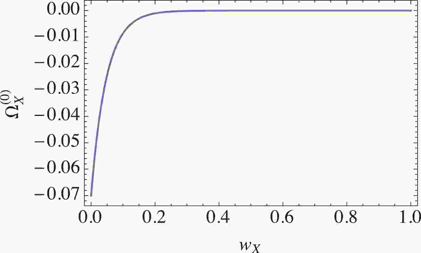
$ r,m,DE,X $ represent radiation, matter, dark energy, and the extra unknown component X, respectively. The notation “$ (0) $ ” denotes the present value at zero redshift. In the$ \Lambda $ CDM model with$ w_{DE} = -1 $ , observational data from the CMB and high-redshifts prefer$ \Omega_m^{(0)} = 0.308 $ ,$ \Omega_r^{(0)} = 9.2 \times 10^{-5} $ , and$ \Omega_{\Lambda = DE}^{(0)} = 0.692 $ , and$ H_{0} = 67.4 \; {\rm km \; s}^{-1}{\rm Mpc}^{-1} $ [14, 43]. We can thus calculate$ H(z) $ at the last-scattering surface ($ z \approx 1100 $ ) to be approximately$ 1.57537\times 10^{6}\; \rm{km \; s}^{-1}{\rm Mpc}^{-1} $ . To address the Hubble tension wherein the value of H at small z is relatively large compared to the Planck value$ H_{0} = 67.4 $ ${\rm{km s}}^{-1}{\rm Mpc}^{-1} $ , we use$ H(z = 1100) = 1.57537\times $ $ 10^{6} \; \rm{km \; s}^{-1} {\rm Mpc}^{-1} $ and$ H_{0} = 74.03\; \rm{km \; s}^{-1}{\rm Mpc}^{-1} $ to determine the physical constraint on the extra unknown component X from Eq. (1). The allowed values of$ w_{X},\Omega_{X}^{(0)} $ are shown in Fig. 1, assuming the simplest case where$ w_{X} $ is constant.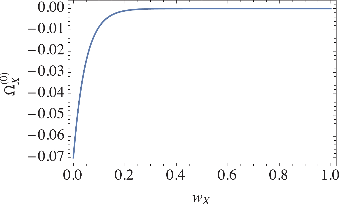
Figure 1. (color online) The relation between
$ \Omega_{X}^{(0)} $ and$ w_{X} $ from Eq. (1) for$ \Omega_m^{(0)} = 0.308 $ ,$ \Omega_r^{(0)} = 9.2 \times 10^{-5} $ , and$ \Omega_{\Lambda = DE}^{(0)} = 1-\Omega_{r}^{(0)}-\Omega_m^{(0)}- \Omega_X^{(0)}, w_{DE} = -1. $ Interestingly, a negative energy density
$ \Omega_{X}^{(0)}<0 $ is required. According to Fig. 1, the negative density cannot be a negative mass ($ w_{X} \approx 0 $ ); otherwise,$ \Omega_{X}^{(0)} $ is too large, i.e.,$ \Omega_{X}^{(0)}\simeq -0.07 $ , and it should have been observed. For$ 1/3\leqslant w_{X}\leqslant 1 $ , however, the amount of the extra component X is very small, i.e.,$ -0.0000636042 \leqslant \Omega_X^{(0)} \leqslant $ $-5.247 \times 10^{-11} $ . Thus, to address the Hubble tension problem, a negative density is required with$ 1/3 \leqslant w_{X} \leqslant 1 $ without modification of the CMB observational data.This particular phenomenological model fails when extrapolated back to early times due to overpopulation of the negative energy. At
$ z = 1100 $ , the density parameter becomes$ \Omega_{X} = -0.23 $ , which should be excluded by the constraints on the power spectrum of the CMB on the early DE. We need a more realistic model with cosmological evolution that suppresses the early DE population and satisfies the early-time constraints from the CMB and the late-time constraints from Baryon Acoustic Oscillations (BAO) and the integrated Sach-Wolfe (iSW) effect.In Section III, a quintom model with two scalars is proposed as a realization of the extra component X. A “phantom” (with a negative kinetic energy term) scalar is assumed to couple to matter, while the other scalar serves as the dark energy that is responsible for the accelerated expansion of the universe. Matter-phantom coupling stabilizes the phantom value by allowing the matter to drag it along, together with the cosmological expansion. The quintessence scalar serves as the DE with negligible contribution in the early times and only increases to dominate in the late epoch. By tuning the model parameters and initial condition, a viable realistic quintom model is achieved that passes some of the early and late time constraints.
-
We consider the quintom action with 2 scalar fields and an interaction between matter fields and one of the scalar fields as follows:
$ \begin{aligned}[b] S =& \int {\rm d}^4 x \sqrt{-g} \left[ \frac{1}{2\kappa^2} R - \frac{1}{2} (\partial \phi)^2 + \frac{1}{2}(\partial \sigma)^2 - V(\phi)\right] \\ & + S_M (g_{\mu\nu}, \sigma, \psi_M) \,, \end{aligned} $

(2) where
$ \kappa^2 = 8 \pi G $ is the inverse of the reduced Planck mass squared. R is the Ricci scalar,$ \phi $ is a quintessence scalar field,$ \sigma $ is a “phantom” scalar field, and$ \psi_M $ is a matter field. We assume that there is only one self-interacting potential of the quintessence scalar field, whereas the “phantom” scalar field is rolling on an effective potential arising from the phantom-matter interaction, as will be explained. Strictly speaking, this$ \sigma $ is not exactly the standard phantom but rather a ghost field since its equation of state is$ P_{\sigma} = \rho_{\sigma}<0 $ . However, here and henceforth, we will refer to it as the phantom field for convenience and also in accordance with the original name quintom (quintessence + phantom). The extra component X is identified using the phantom field$ \sigma $ in this model. It shoud be noted that the quintom model a has negative kinetic energy term in the Lagrangian. Thus, the phantom scalar field encounters a quantum instability problem of its own. In our model, however, the total energy density of all components in the universe is always positive, and the evolution of the universe always obeys the positive energy condition.By varying the action with respect to
$ g^{\mu\nu} $ , we obtain the equation of motion$ R_{\mu\nu} - \frac{1}{2}g_{\mu\nu} R = \kappa^2 (T_{\mu\nu}^{(M)} + T_{\mu\nu}^{(\phi)} + T_{\mu\nu}^{(\sigma)}) \,, $

(3) where
$ T_{\mu\nu}^{(M)} $ is an energy-momentum tensor of non-relativistic matter and radiation. The energy-momentum tensors of the quintessence scalar field and the phantom scalar field are given by:$T_{\mu \nu }^{(\phi )} = {\partial _\mu }\phi {\partial _\nu }\phi + {g_{\mu \nu }}\left( { - \frac{1}{2}{{(\partial \phi )}^2} - V(\phi )} \right) ,$

(4) $T_{\mu \nu }^{(\sigma )} = - {\partial _\mu }\sigma {\partial _\nu }\sigma + {g_{\mu \nu }}\left( {\frac{1}{2}{{(\partial \sigma )}^2}} \right),$

(5) respectively. Using the flat Friedmann-Lemaître-Robertson-Walker (FLRW) metric,
$ {\rm d}s^2 = - {\rm d}t^2 + a^2 (t){\rm d} {x}^2 $ , and assuming$ \phi = \phi(t) $ and$ \sigma = \sigma(t) $ , we obtain the Friedmann equations,$3{H^2} = {\kappa ^2}({\rho _m} + {\rho _r} + {\rho _\phi } + {\rho _\sigma }),$

(6) $3{H^2} + 2\dot H = {\kappa ^2}( - {P_m} - {P_r} - {P_\phi } - {P_\sigma }).$

(7) $ \rho_m $ ,$ \rho_r $ ,$ P_m $ , and$ P_r $ are the energy densities and pressures of non-relativistic matter and radiation, respectively. The notation “$ \; ^. \; $ ” denotes a derivative with respect to time. The energy densities and pressures of the scalar fields are${\rho _\phi } = \frac{1}{2}{\dot \phi ^2} + V(\phi ){\mkern 1mu} ,\;\;\;{\rho _\sigma } = - \frac{1}{2}{\dot \sigma ^2},$

(8) ${P_\phi } = \frac{1}{2}{\dot \phi ^2} - V(\phi ) ,\;\;\;{P_\sigma } = - \frac{1}{2}{\dot \sigma ^2}.$

(9) We can then define an equation of the state parameter of the dark energy and an effective equation of state parameter as
${w_{DE}} \equiv \frac{{{P_\phi } + {P_\sigma }}}{{{\rho _\phi } + {\rho _\sigma }}} = \frac{{\dfrac{1}{2}{{\dot \phi }^2} - \dfrac{1}{2}{{\dot \sigma }^2} - V(\phi )}}{{\dfrac{1}{2}{{\dot \phi }^2} - \dfrac{1}{2}{{\dot \sigma }^2} + V(\phi )}},$

(10) ${w_{{\rm{eff}}}} \equiv \frac{{{P_\phi } + {P_\sigma } + {P_m} + {P_r}}}{{{\rho _\phi } + {\rho _\sigma } + {\rho _m} + {\rho _r}}} = - 1 - \frac{2}{3}\frac{{\dot H}}{{{H^2}}}.$

(11) It should be noted that
$ w_{DE} $ in this section and henceforth is contributed by both scalar fields, which is different from the$ w_{DE} $ in the Section II. For each scalar field, the equation of state parameters are$ w_{\phi} = \frac{P_{\phi}}{\rho_{\phi}} = \frac{\dfrac{1}{2}\dot \phi^2 - V(\phi)}{\dfrac{1}{2}\dot \phi^2 + V(\phi)} \,, \; \; \; w_{\sigma} = \frac{P_{\sigma}}{\rho_{\sigma}} = +1 \,. $

(12) It should be noted that
$ \rho_{\sigma} $ is negative, and$ w_{\sigma} $ is always equal to +1. This is crucial in resolving the Hubble tension problem, which will be shown in the Section IV.We assume that there is only an interaction between the matter field and the phantom field, i.e.,
$ \nabla_{\mu} T^{\mu (\phi)}_{\nu} = 0 $ . In this work we consider an interaction of the form${\nabla _\mu }T_\nu ^{\mu (M)} = \kappa \delta {T_M}{\nabla _\nu }\sigma ,$

(13) ${\nabla _\mu }T_\nu ^{\mu (\sigma )} = - \kappa \delta {T_M}{\nabla _\nu }\sigma ,$

(14) where
$ T_M = -\rho_M + 3P_M $ , and$ \delta $ is a dimensionless constant. This is a conformal interaction form that arises in many scalar-tensor theories after performing a conformal transformation to the Einstein frame [44, 45]. Hence, the continuity equations are${\dot \rho _m} + 3H{\rho _m} = \kappa \delta {\rho _m}\dot \sigma ,$

(15) ${\dot \rho _\sigma } + 3H({\rho _\sigma } + {P_\sigma }) = - \kappa \delta {\rho _m}\dot \sigma ,$

(16) ${\dot \rho _\phi } + 3H({\rho _\phi } + {P_\phi }) = 0,$

(17) ${\dot \rho _r} + 4H{\rho _r} = 0.$

(18) Substituting for the energy density and pressure of each scalar field, we obtain the equations of motion
$ \ddot \sigma + 3H \dot \sigma = \kappa \delta \rho_m \,, $

(19) $ \ddot \phi + 3H \dot \phi + V_{,\phi} = 0 \,. $

(20) The right-hand-side (RHS) of the equation of motion of the phantom scalar field acts as an effective potential. This is similar to the effective potential in chameleon or symmetron gravity [46-48]
-
We will use a dynamical system approach to study the cosmological scenarios of the quintom dark energy model based on the behaviour of their fixed points. First, the dimensionless dynamic variables are defined as follows;
$ \begin{aligned}[b]& x_1 \equiv \frac{\kappa \dot\phi}{\sqrt{6}H} \,, \quad x_2 \equiv \frac{\kappa \sqrt{V(\phi)}}{\sqrt{3}H} \,, \\& x_3 \equiv \frac{\kappa \dot\sigma}{\sqrt{6}H} \,, \quad x_4 \equiv \frac{\kappa \sqrt{\rho_r}}{\sqrt{3}H} \,. \end{aligned} $

(21) According to the Friedmann Eq. (6), the density parameters in terms of the dynamic variables are
${\Omega _m} = 1 - x_1^2 - x_2^2 + x_3^2 - x_4^2,$

(22) ${\Omega _r} = x_4^2,$

(23) ${\Omega _{DE}} = x_1^2 + x_2^2 - x_3^2,$

(24) ${\Omega _\phi } = x_1^2 + x_2^2,$

(25) ${\Omega _\sigma } = - x_3^2,$

(26) where
$ \Omega_m \equiv \kappa^2 \rho_m / 3H^2 $ . In addition, the equation of states are${w_{DE}} = \frac{{x_1^2 - x_2^2 - x_3^2}}{{x_1^2 + x_2^2 - x_3^2}},$

(27) ${w_\phi } = \frac{{x_1^2 - x_2^2}}{{x_1^2 + x_2^2}},$

(28) ${w_\sigma } = 1,$

(29) ${w_{{\rm{eff}}}} = x_1^2 - x_2^2 - x_3^2 + \frac{{x_4^2}}{3}.$

(30) In the last equation , we used the second Friedmann Eq. (7), which leads to
$ \frac{\dot H}{H^2} = - \frac{1}{2}\left(3 + 3x_1^2 - 3x_2^2 - 3x_3^2 + x_4^2 \right) \,. $

(31) Differentiating the dynamic variables with respect to N, where
$ N = \ln a $ is an e-folding number, we obtain a set of autonomous equations:$\frac{{{\rm d}{x_1}}}{{{\rm d}N}} = \frac{{\sqrt 6 }}{2}{\lambda _\phi }x_2^2 - 3{x_1} - {x_1}\frac{{\dot H}}{{{H^2}}},$

(32) $\frac{{{\rm d}{x_2}}}{{{\rm d}N}} = - \frac{{\sqrt 6 }}{2}{\lambda _\phi }{x_1}{x_2} - {x_2}\frac{{\dot H}}{{{H^2}}},$

(33) $ \frac{{\rm d}x_3}{{\rm d}N} = \frac{\sqrt{6}}{2}\delta (1-x_1^2 -x_2^2 + x_3^2 -x_4^2) - 3x_3 - x_3 \frac{\dot H}{H^2} \,, $

(34) $\frac{{{\rm d}{x_4}}}{{{\rm d}N}} = - 2{x_4} - {x_4}\frac{{\dot H}}{{{H^2}}},$

(35) where
$ \lambda_{\phi} \equiv - V_{,\phi} / \kappa V $ . For an exponential form of a potential, i.e.,$ V(\phi) = V_0 {\rm e}^{- \kappa \lambda_{\phi} \phi} $ ,$ \lambda_{\phi} $ is a constant, and the autonomous equations are closed.The fixed points of the system can be obtained by setting
$ {\rm d}x_1/{\rm d}N = {\rm d}x_2/{\rm d}N = {\rm d}x_3/{\rm d}N = {\rm d}x_4/{\rm d}N = 0 $ . They are shown in Appendix A. The dynamic variables$ x_2 $ and$ x_4 $ are always positive, whereas$ x_1 $ and$ x_3 $ can be positive or negative depending on the signs of$ \dot\phi $ or$ \dot\sigma $ . We are only interested in the case where$ \lambda_{\phi} > 0 $ (an exponential decay) and$ \delta > 0 $ . For these fixed points, the density parameters and equation of state parameters are presented in Table 1.$ \Omega_m $ 

$ \Omega_r $ 

$ \Omega_{DE} $ 

$ w_{DE} $ 

$ w_{\rm eff} $ 

(a) 0 0 1 1 1 (b) 0 1 0 − $\dfrac{1}{3}$ 

(c) $-\dfrac{1}{3\delta^2}$ 

$1+\dfrac{1}{2\delta^2}$ 

$- \dfrac{1}{6\delta^2}$ 

1 $\dfrac{1}{3}$ 

(d) $1+ \dfrac{2\delta^2}{3}$ 

0 $- \dfrac{2\delta^2}{3}$ 

1 $- \dfrac{2\delta^2}{3}$ 

(e) 0 $1 - \dfrac{4}{\lambda_{\phi}^2}$ 

$\dfrac{4}{\lambda_{\phi}^2}$ 

$\dfrac{1}{3}$ 

$\dfrac{1}{3}$ 

(f) $- \dfrac{1}{3\delta^2}$ 

$1 + \dfrac{1}{2\delta^2} - \dfrac{4}{\lambda_{\phi}^2}$ 

$- \dfrac{1}{6\delta^2} + \dfrac{4}{\lambda_{\phi}^2}$ 

$\dfrac{8\delta^2 - \lambda_{\phi}^2}{24\delta^2 - \lambda_{\phi}^2}$ 

$\dfrac{1}{3}$ 

(g) 0 0 1 $-1 + \dfrac{\lambda_{\phi}^2}{3}$ 

$-1 + \dfrac{\lambda_{\phi}^2}{3}$ 

(h) $\dfrac{(\lambda_{\phi}^2 -3)(3\lambda_{\phi}^2 + 2\delta^2 (\lambda_{\phi}^2 - 6))}{3(\lambda_{\phi}^2 - 2\delta^2)^2}$ 

0 $\dfrac{12\delta^4 + 9\lambda_{\phi}^2 - 2\delta^2 (18 - 3 \lambda_{\phi}^2 + \lambda_{\phi}^4)}{3(\lambda_{\phi}^2 - 2\delta^2)^2}$ 

$\dfrac{2\delta^2 (2\delta^2 - \lambda_{\phi}^2)(\lambda_{\phi}^2 - 3)}{12\delta^4 + 9 \lambda_{\phi}^2 - 2 \delta^2 (18 - 3\lambda_{\phi}^2 + \lambda_{\phi}^4)}$ 

$\dfrac{2\delta^2 (\lambda_{\phi}^2 - 3)}{6\delta^2 - 3\lambda_{\phi}^2}$ 

Table 1. Density and equation of state parameters of each fixed point.
In the next section, the stability of each fixed point will beexamined by considering its corresponding eigenvalues.
-
The eigenvalues of each fixed point in Table A1 are as follows (the definition of eigenvalues is presented in Appendix B).
$ x_1 $ 

$ x_2 $ 

$ x_3 $ 

$ x_4 $ 

existence (a) $ x_1^2 - x_3^2 = 1 $ 

0 0 $ x_1^2 - x_3^2 = 1 $ 

(b) 0 0 0 1 All (c) 0 0 $- \dfrac{1}{\sqrt{6}\delta}$ 

$\sqrt{1+ \dfrac{1}{2\delta^2} }$ 

All (d) 0 0 $\sqrt{\dfrac{2}{3} }\delta$ 

0 All (e) $\dfrac{2\sqrt{6} }{3\lambda_{\phi} }$ 

$\dfrac{2\sqrt{3} }{3\lambda_{\phi} }$ 

0 $\sqrt{1 - \dfrac{4}{\lambda_{\phi}^2} }$ 

$ \lambda_{\phi} \geqslant 2 $ 

(f) $ \dfrac{2\sqrt{6}}{3\lambda_{\phi}} $ 

$ \dfrac{2\sqrt{3}}{3\lambda_{\phi}} $ 

$ -\dfrac{1}{\sqrt{6}\delta} $ 

$ \dfrac{\sqrt{\lambda_{\phi}^2 + 2\delta^2 (\lambda_{\phi}^2 - 4)}}{\sqrt{2}\delta \lambda_{\phi}} $ 

$ 0< \lambda_{\phi}< 2\,, 0< \delta \leqslant \sqrt{\dfrac{\lambda_{\phi}^2}{8 - 2 \lambda_{\phi}^2}} $ 

or$ \lambda_{\phi} \geqslant 2\,, \delta> 0 $ 

(g) $ \dfrac{\lambda_{\phi}}{\sqrt{6}} $ 

$ \sqrt{1 - \dfrac{\lambda_{\phi}^2}{6}} $ 

0 0 $ 0< \lambda_{\phi} \leqslant \sqrt{6} $ 

(h) $ \dfrac{(3 - 2 \delta^2)\lambda_{\phi}}{\sqrt{6} (\lambda_{\phi}^2 - 2 \delta^2)} $ 

$ \sqrt{\dfrac{-36\delta^2 + 9\lambda_{\phi}^2 - 4 \delta^4 (\lambda_{\phi}^2 - 6)}{6 (\lambda_{\phi}^2 - 2 \delta^2)^2}} $ 

$ - \sqrt{\frac{2}{3}} \dfrac{\delta (\lambda_{\phi}^2 - 3)}{2\delta^2 -\lambda_{\phi}^2} $ 

0 $ \delta> 0 \,, \lambda_{\phi} = \sqrt{3} $ 

or$\delta > 0 \,, 0 < \lambda_{\phi} \leqslant \sqrt{3} \,, \sqrt{\dfrac{6\lambda_{\phi}^2}{6 - \lambda_{\phi}^2} } \geqslant 2 \delta$ 

or$0 < \delta \leqslant \sqrt{\dfrac{3}{2} } \,, \lambda_{\phi} > \sqrt{3}$ 

or$ 0< \lambda_{\phi}< \sqrt{3} \,, 2\delta \geqslant \sqrt{6} $ 

or$ \sqrt{3}< \lambda_{\phi}< \sqrt{6} \,, \sqrt{\dfrac{6\lambda_{\phi}^2}{6 - \lambda_{\phi}^2}} \leqslant 2\delta $ 

Table A1. Fixed points of the autonomous equations (32)-(35).
-
The eigenvalues of the fixed point are
$ \mu_{(\rm a)} = 1\,, 0\,, 3\pm \sqrt{6} \, \delta \sqrt{x_1^2-1}\,, 3-\sqrt{\frac{3}{2}} \lambda_{\phi} x_1 \,. $

(36) Although the sign
$ \pm $ depends on the roots of the condition$ x_1^2 - x_3^2 = 1 $ , the fixed point is either a saddle or an unstable point. Since this fixed point does not match with any known cosmological era, it is no longer considered. -
The eigenvalues of the fixed point (b), (c), (e), and (f) are given by
${\mu _{(\rm b)}} = 2{\mkern 1mu} , - 1{\mkern 1mu} , - 1{\mkern 1mu} ,1.$

(37) ${\mu _{(\rm c)}} = - 1{\mkern 1mu} ,2{\mkern 1mu} , - \frac{1}{2} \pm \frac{1}{2}\sqrt { - \left( {\frac{2}{{{\delta ^2}}} + 3} \right)} ,$

(38) ${\mu _{(\rm e)}} = - 1{\mkern 1mu} ,1{\mkern 1mu} , - \frac{1}{2} \pm \sqrt {\frac{{16}}{{\lambda _\phi ^2}} - \frac{{15}}{4}} ,$

(39) $\begin{aligned}[b]{\mu _{(\rm f)}} =& - \frac{1}{2} \pm \frac{1}{{2{\delta ^2}\lambda _\phi ^2}}\sqrt { - {\delta ^2}\lambda _\phi ^4 + {\delta ^4}(32\lambda _\phi ^2 - 9\lambda _\phi ^4) + \sqrt {{\delta ^4}\lambda _\phi ^4(\lambda _\phi ^4 + 4{\delta ^4}{{(16 - 3\lambda _\phi ^2)}^2} - 4{\delta ^2}\lambda _\phi ^2(16 + 3\lambda _\phi ^2))} } ,\\& - \frac{1}{2} \pm \frac{1}{{2{\delta ^2}\lambda _\phi ^2}}\sqrt { - {\delta ^2}\lambda _\phi ^4 + {\delta ^4}(32\lambda _\phi ^2 - 9\lambda _\phi ^4) - \sqrt {{\delta ^4}\lambda _\phi ^4(\lambda _\phi ^4 + 4{\delta ^4}{{(16 - 3\lambda _\phi ^2)}^2} - 4{\delta ^2}\lambda _\phi ^2(16 + 3\lambda _\phi ^2))} } .\end{aligned}$

(40) Therefore, the fixed point (b), (c), and (e) are saddle points. For the point (f), we can understand the behaviour of the fixed point when we set the value of
$ \lambda_{\phi} $ and$ \delta $ . -
For the fixed points (d) and (h), their corresponding eigenvalues are
${\mu _{(\rm d)}} = - \frac{3}{2} - {\delta ^2}{\mkern 1mu} , - \frac{3}{2} - {\delta ^2}{\mkern 1mu} , - \frac{1}{2} - {\delta ^2}{\mkern 1mu} ,\frac{3}{2} - {\delta ^2},$

(41) $ \begin{aligned}[b] \mu_{(\rm h)} =& \frac{\lambda_{\phi}^2 + 2\delta^2 (\lambda_{\phi}^2 - 4)}{4\delta^2 - 2 \lambda_{\phi}^2} \,, \frac{3\lambda_{\phi}^2 + 2\delta^2 (\lambda_{\phi}^2 - 6)}{4\delta^2 - 2 \lambda_{\phi}^2} \,, \frac{1}{4(\lambda_{\phi}^2 - 2\delta^2)^2} \left(-3\lambda_{\phi}^4 - 2\delta^2 \lambda_{\phi}^2 (\lambda_{\phi}^2 - 9) + 4 \delta^4 (\lambda_{\phi}^2 - 6) \right. \\& \left. \pm \sqrt{3(\lambda_{\phi}^2 - 2 \delta^2)^2(72 \lambda_{\phi}^2 - 21 \lambda_{\phi}^4 + 4\delta^2 (-72 + 18 \lambda_{\phi}^2 + \lambda_{\phi}^4) + 4\delta^4 (60 - 28 \lambda_{\phi}^2 + 3\lambda_{\phi}^4))}\right) \,. \end{aligned}$

(42) The fixed point (d) is stable when
$ \delta^2 > \frac{3}{2} $ , whereas it is a saddle point when$ \delta^2 < \frac{3}{2} $ . For the fixed point (h), the eigenvalues can be understood once we set the values of$ \lambda_{\phi} $ and$ \delta $ . -
The eigenvalues of the fixed point (g) are
$ \mu_{(\rm g)} = \frac{1}{2} (\lambda_{\phi}^2 - 6) \,, \frac{1}{2} (\lambda_{\phi}^2 - 6)\,, \frac{1}{2} (\lambda_{\phi}^2 - 4) \,, \lambda_{\phi}^2 - 3 \,. $

(43) Thus, the fixed point is stable when
$ \lambda_{\phi}^2 < 3 $ . For the point (h), it is the same as the previous case. -
In this section, the autonomous Eqs. (32)-(35) are solved numerically, wherein we set
$ \lambda_{\phi} = 0.1 $ and$ \delta = 0.113 $ . This choice lies within the range of values that satisfy the fixed-points scenario$ \lambda_{\phi}<\sqrt{3},\delta<\sqrt{3/2} $ discussed previously and the condition$ w_{\rm eff}<-1/3 $ at the fixed point (g) which gives$ \lambda_{\phi}<\sqrt{2} $ for accelerated expansion. By tuning the model parameters and the initial condition, we can obtain the Hubble parameter in the desired range of values, namely$ H_{0} \approx 74 $ km s$ ^{-1} $ Mpc$ ^{-1} $ , to address the Hubble tension. Since a viable cosmology requires a sufficiently long period of a radiation dominated era, we choose the initial point of the numerical solution to be deep into the radiation epoch at$ z = 9.74811 \times 10^5 $ corresponding to$ N = -\ln(1+z) = -13.79 $ , to guarantee a long radiation epoch. The cosmological evolution is insensitive to the choice of the initial value of N, e.g., setting$ N = -13.81 $ would yield indistinguishable results provided that we define the present-day$ N_{0} $ such that$ \Omega_{m}^{(0)} $ has the same value. When we change the initial value of N, the present-day value$ N_{0} $ at some fixed choice of$ (\Omega_{m}^{(0)},\Omega_{r}^{(0)}) $ will shift accordingly. The overall cosmological evolution remains the same with the physical redshift defined as$ N-N_{0} = -\ln(1+z) $ . Evolutions of the density parameters and equation of state parameters are shown in Fig. 2.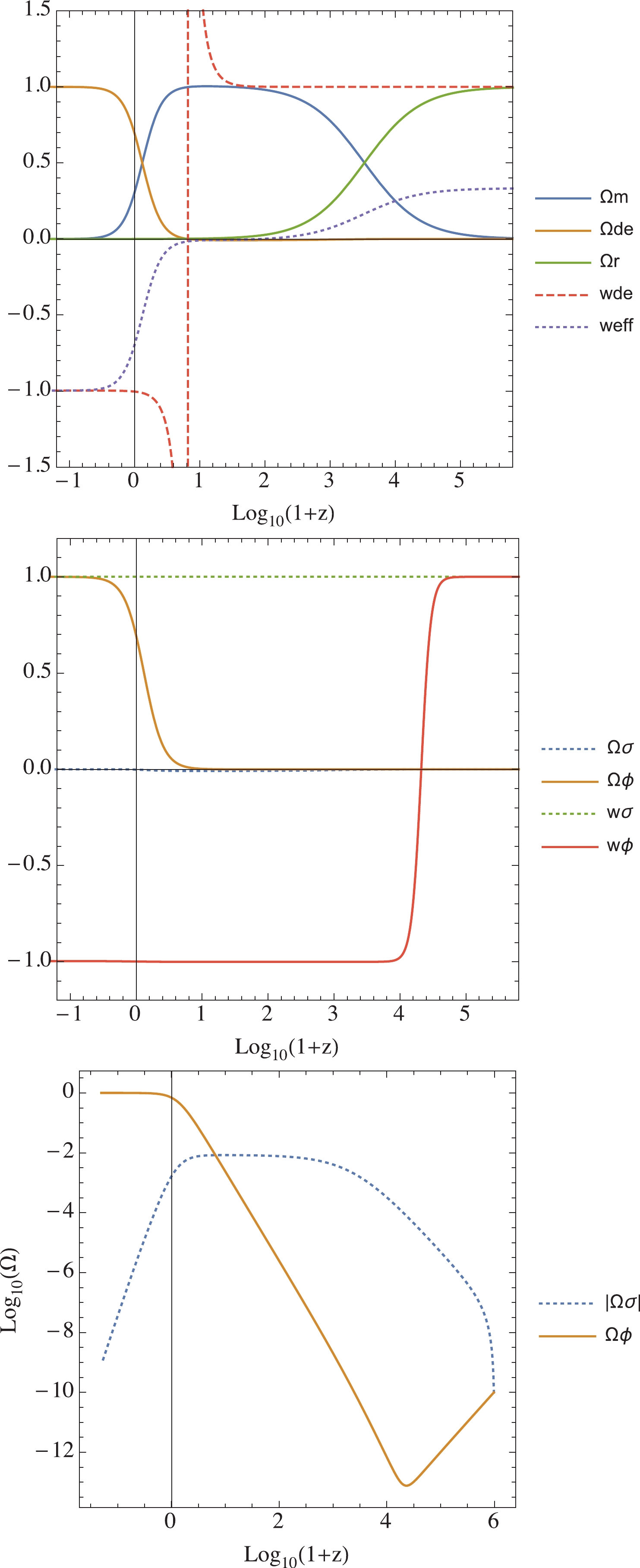
Figure 2. (color online) Evolutions of the density and equation of state parameters according to Eqs. (22)-(30), where initial conditions are
$ x_1 = 1 \times 10^{-5} $ ,$ x_2 = 1 \times 10^{-10} $ ,$ x_3 = 1 \times 10^{-5} $ , and$ x_4 = 0.9983 $ at$ z = 9.74811 \times 10^5\; (N = -13.79) $ .Figure 2 demonstrates a viable cosmological scenario wherein the universe evolves from the radiation dominated era to the matter dominated epoch, followed by the late-time accelerated expansion. Since
$ \lambda_{\phi} = 0.1 $ and$ \delta = 0.113 $ , the fixed points (e), (f), and (h) do not exist, whereas the fixed point (c) yields$ \Omega_r \approx 40 $ , which is too large. Since we are interested in$ \Omega_r \approx 1 $ , we choose the initial condition to be close to the fixed point (b). The matter dominated era is automatically point (d), and the accelerated expansion is the point (g). Therefore, the cosmological viable evolution is$ {\rm (b)} \; \; \rightarrow \; \; {\rm (d)} \; \; \rightarrow \; \; {\rm (g)} \,. $

(44) According to the middle figure of Fig. 2, the density of the phantom scalar field is negative, and
$ w_{\sigma} = 1 $ as desired, whereas the density of dark energy (quintessence + phantom) increases at late-time. We can obtain the evolution of the Hubble parameter by integrating Eq. (31),$ \begin{aligned}[b] H(N) =& C \exp\left[\frac{1}{2} \left(-3 N - 3 \int x_1^2 {\rm d}N + 3\int x_2^2 {\rm d}N \right.\right. \\ & \left.\left. + 3 \int x_3^2 {\rm d}N - \int x_4^2 {\rm d}N\right)\right] \,, \end{aligned} $

(45) where C is a constant of integration, which can be obtained by comparing the preceding equation to the Hubble parameter from the
$ \Lambda $ CDM at the last-scattering surface.$ x_1 $ ,$ x_2 $ ,$ x_3 $ , and$ x_4 $ are obtained from numerical solutions with the same initial conditions used in Fig. 2. We set$ H_0 = 67.4\; {\rm km \; s}^{-1}{\rm Mpc}^{-1} $ to find the Hubble parameter at$ z = 1100 $ using the$ \Lambda $ CDM model; then, we start the evolution in the quintom model using this value of$ H(1100) $ . The evolution of the Hubble parameter of the quintom compared to that of the$ \Lambda $ CDM is shown in Fig. 3.
Figure 3. (color online) Top figure represents the evolution of the Hubble parameters at late-time, while the bottom figure represents the percent deviation from
$ \Lambda $ CDM from the last-scattering surface to the present.In Fig. 3, the Hubble parameter of the quintom model decreases at a slightly different rate compared to the
$ \Lambda $ CDM, where we obtain$ H_0 = 73.356\; {\rm km \; s}^{-1}{\rm Mpc}^{-1} $ at the present time. The data of$ H(z) $ are from Ref. [49]. Remarkably, the Hubble tension is alleviated. It should be noted that the value of$ H_0 $ depends on the initial conditions, and the values of$ \lambda_{\phi} $ and$ \delta $ can be tuned to yield superior precision compared to the observational results, as will be shown.The cosmological parameters at the present time that were obtained based on numerical simulations are presented in Table 2. These parameters correspond to the redshift at
$ z = 0 $ in Figs. 2 and 3.$ \Omega_m^{(0)} $ 

$ \Omega_{DE}^{(0)} $ 

$ \Omega_r^{(0)} $ 

$ \Omega_{\sigma}^{(0)} $ 

$ \Omega_{\phi}^{(0)} $ 

0.3078 0.69211 $ 7.66\times 10^{-5} $ 

−0.00164 0.69376 $ w_{DE} $ 

$ w_{\rm eff} $ 

$ w_{\sigma} $ 

$ w_{\phi} $ 

−1.003 −0.694 1 −0.9985 Table 2. Cosmological parameters at the present time from the quintom model
The motivation of this work is to modify the standard
$ \Lambda $ CDM model such that the early-time parameters are mostly unchanged. In contrast, an additional phantom field only exhibits small effects, but the accumulative change in the value of$ H_{0} $ is significant. We thus explore the parameter space of the coupled quintom model with respect to$ H_{0} $ , where values of$ \lambda_{\phi}<\sqrt{2}, \delta<\sqrt{3/2} $ are required for a late-time accelerated expansion. In Fig. 4, the contour of constant$ H_{0} $ is shown with respect to phantom-matter coupling$ \delta $ and the present-day matter density parameter$ \Omega_{m}^{(0)} $ , where the superscript is suppressed. The value of$ H_{0} $ depends not only on$ \Omega_{m}^{(0)} $ but also on the coupling$ \delta $ . Notably, the present-day Hubble parameter depends weakly on$ \lambda_{\phi} $ , which governs the quintessence evolution.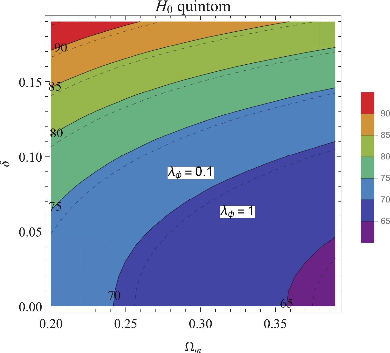
Figure 4. (color online) Parameter space of the coupled quintom model for fixed
$\lambda_{\phi}$ , the number on each pair of contour is the value of the corresponding$H_{0}$ . The solid (dashed) line represents contours with$\lambda_{\phi}=0.1\;(1)$ respectively. The parameter space changes only slightly with$\lambda_{\phi}$ .To examine the viability of the coupled quintom model, we plot the contour of each value of
$ H_{0} $ in the parameter space with respect to the constraints$\Omega_{m}^{(0)} = 0.308, $ $ \Omega_{\gamma}^{(0)} = 5.38\times 10^{-5}, N_{\rm eff} = 3.13 $ in Fig. 5. The value of$ H_{0} $ varies significantly with$ \delta $ but is relatively insensitive to the parameter$ \lambda_{\phi} $ . For a given value of$ \Omega_{m}^{(0)} $ , the quintom model presents a range of possibilities for$ H_{0} $ , starting from the value corresponding to the$ \Lambda $ CDM model, to higher values. Interestingly, this unique property of the coupled quintom model makes it a good candidate to resolve the Hubble tension problem. For$ H_{0}\simeq 74 $ km s$ ^{-1} $ Mpc$ ^{-1} $ , it corresponds to the range$ \delta = 0.11-0.12 $ .
Figure 5. (color online) Parameter space of the coupled quintom model under the condition
$\Omega_{m}^{(0)}=0.308,\;$ $\Omega_{\gamma}^{(0)}=5.38\times 10^{-5}, \; N_{\rm eff}=3.13$ ; the number on each contour is the value of the corresponding$H_{0}$ . Region with small$(\lambda_{\phi}, \delta)$ gives$H_{0}\simeq 67- 68\;{\rm km \;s}^{-1}{\rm Mpc}^{-1}$ , close to the value of the$\Lambda$ CDM model. -
In this section, we compare the cosmology data obtained using the quintom model with observational data, particularly for the CMB constraints from the early time
$ z\geqslant z_{\rm{dec}} $ , BAO constraints that originate from$ z = z_{\rm{drag}} $ , and Type Ia Supernovae (SN) from the late time$ z\lesssim 2.3 $ . The Planck constraints are determined from the base$ \Lambda $ CDM model. Therefore, certain constraints are not necessarily valid for other models. Since the Hubble tension arises due to the more accurately measured luminosity of SN Ia resulting in a larger value of$ H_{0} $ compared to the value implied from the Planck CMB measurement based on the assumption of a$ \Lambda $ CDM model, some of the constraints that depend on the cosmological model could be relaxed, e.g., the constraint$ \Omega_{m}^{(0)}h^{2} = 0.14170\pm 0.00097 $ [14]. The benchmark quintom model we are considering is based on the choice of parameters that would suppress the difference in the iSW effects in the late time for the$ \Lambda $ CDM, by tuning the initial conditions and model parameters so that$ \Omega_{DE}^{(0)}, \Omega_{m}^{(0)} $ are as close to the best-fit values of the$ \Lambda $ CDM model as possible. The cosmological parameters are given in Table 2 and were obtained from the initial conditions$ x_1 = 1 \times 10^{-5} $ ,$ x_2 = 1 \times 10^{-10} $ ,$ x_3 = 1 \times 10^{-5} $ , and$ x_4 = 0.9983 $ at$ N = -13.79 $ , and the model parameters$ \lambda_{\phi} = 0.10, \delta = 0.113 $ . Another example of evidence for this benchmark is the excellent fit with the SN Ia data. Subsequent analysis reveals that$ \Omega_{m}^{(0)}\simeq 0.308-0.315 $ is prefered for the quintom model with$ H_{0}\simeq 73.4 $ km s$ ^{-1} $ Mpc$ ^{-1} $ . However, this yields$ \Omega_{m}^{(0)}h^{2} = 0.166-0.170 $ . Here and henceforth, we refer to this quintom model as Quintom I.Starting with the SN Ia observations, we use observational data between the magnitude
$ m_{B} $ and redshift parameter of Type Ia Supernovae from Ref. [50] (Pantheon analysis) and take the absolute magnitude M to be a fitting parameter that is unique for the entire set of data. To focus only on the essential differences between the quintom and$ \Lambda $ CDM models, the statistical analysis is simplified to contain only one parameter, M, which is assumed to include not only the absolute magnitude but also the combined effects of other nuisance parameters such as the stretch and color measure of the SN Ia data (for more careful analyses including stretch and color measurements, see e.g. Refs. [50-52]). The distance modulus$ \mu_{L} $ is related to the observable$ m_{B} $ and the luminosity distance$ d_{L} $ by${\mu _L} = {m_B} - M = 5{\log _{10}}\left( {\frac{{{d_L}}}{{{\rm{Mpc}}}}} \right) + 25.$

(46) The luminosity distance contains information about the evolution of the universe via the Hubble parameter,
${d_L} = c(1 + z)\int_0^z \; \frac{{{\rm d}z}}{{H(z)}},$

(47) where
$ H(z) $ can be calculated from Eq. (1) and Eq. (45) depending on the model. For the$ \Lambda $ CDM and other non-coupled phenomenological models, Eq. (1) will suffice. However, our quintom model with phantom-matter coupling can be more accurately calculated using Eq. (45). Figure 6 shows a comparison between the theoretical models and the Supernovae observational data. The$ \Lambda $ CDM parameters were chosen to be$ h = 67.4, \Omega_{m}^{(0)} = 0.308 $ . The fits of all 1048 data points for$ z<2.3 $ and the 211 data points for a small redshift$ z<0.1 $ are presented in Fig. 6, for which the two models appear to be degenerate on a single line. We define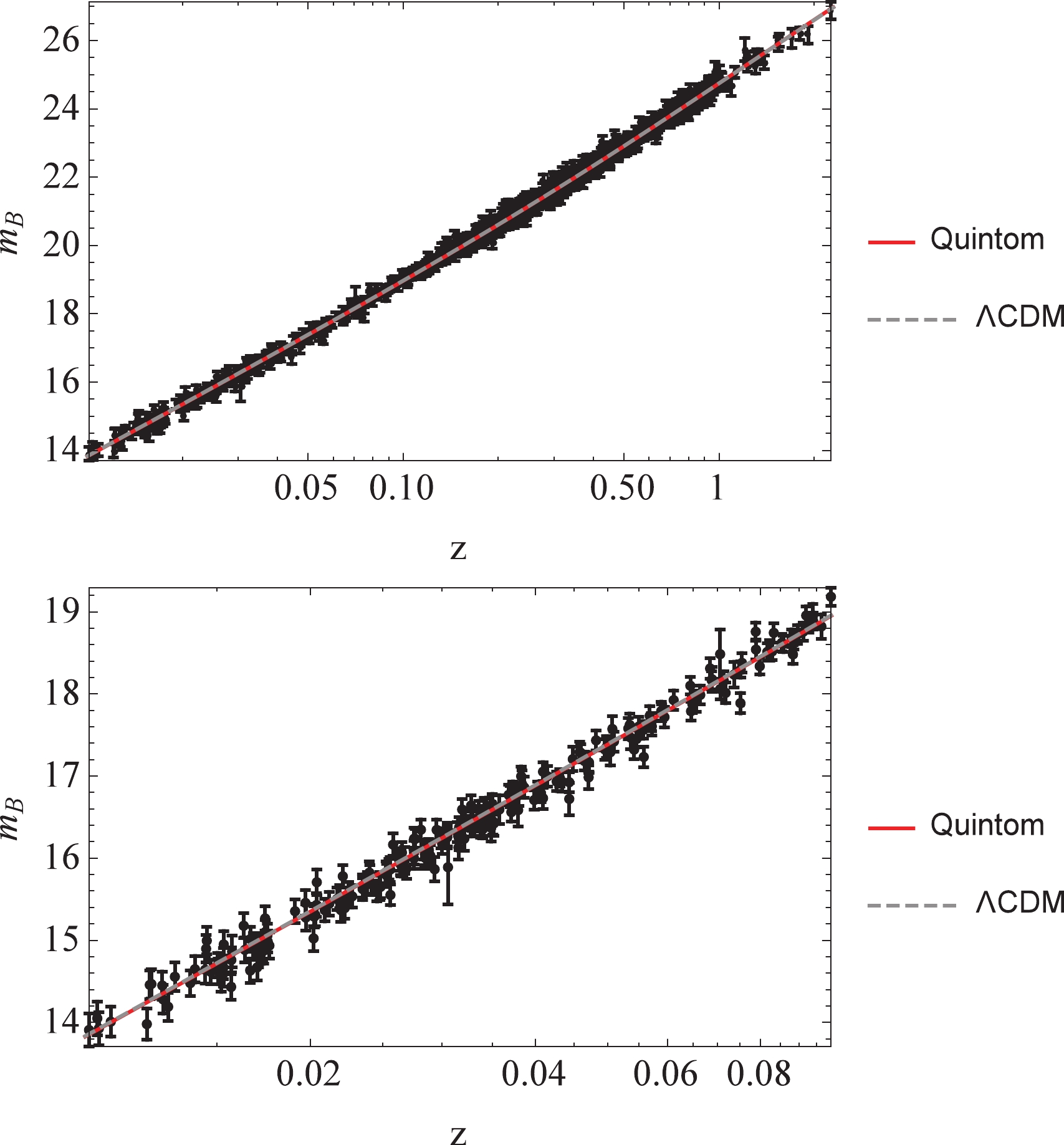
Figure 6. (color online) Comparison between Type Ia Supernovae data from Ref. [50] and theoretical models:
$ \Lambda $ CDM and quintom.$ \chi^{2}\equiv \Delta \vec{m}^{T}C^{-1}\Delta \vec{m}, $

(48) where
$ \Delta \vec{m}_{i} = m_{B,i}^{\rm obs}-m_{B,i}^{\rm th}\; (i = 1 $ to number the data points),$ C = D_{\rm stat}+C_{\rm sys} $ . The uncertainty matrix C contains the diagonal statistical matrix$ D_{\rm stat} $ and the off-diagonal covariance matrix$ C_{\rm sys} $ ; see Ref. [50]. For all 1048 data points, the chi-square values of the fitting are$ \chi^{2}_{\Lambda \rm{CDM}} = 1027.07 $ for$ M = -19.429 $ and$ \chi^{2}_{\rm{quin}} = 1026.74 $ for$ M = -19.247 $ . For the 211 low-redshift data points,$ \chi^{2}_{\Lambda \rm{CDM}} = 217.804 $ for$ M = -19.442 $ and$ \chi^{2}_{\rm{quin}} = 217.784 $ for$ M = -19.257 $ ①. The quintom model clearly yields an equally good fit to the$ \Lambda $ CDM.The degenerate plots of both models are the result of the same values for matter and dark energy densities for late times between the two models (since we tune the benchmark quintom model such that this is the case), while the difference in
$ H_{0} $ is compensated by the different fitting values of the absolute magnitude M. The quintom model prefers the absolute magnitude to be approximately -19.25 to -19.26, whereas$ \Lambda $ CDM prefers$ |M|\simeq 19.43-19.44 $ . The quintom model gives a value for the best-fit M, whichis very close to the central value $ \overline{M} = -19.25\pm 0.20 $ given in Ref. [53]. However, the error bar is sufficiently large to accommodate the best-fit M of$ \Lambda $ CDM. More precise measurement of the absolute magnitude of the SN Ia could potentially facilitate the identification of the superior model .Next, we consider the acoustic peaks of the CMB in the quintom model. Generically, the multipole
$ \ell_{A} $ of the acoustic peaks in the CMB is given by$ \ell_{A} = \frac{\pi}{\theta_{A}} = \pi\frac{(1+z_{\rm dec})d_{A}(z_{\rm dec})}{r_{s}(z_{\rm dec})}, $

(49) where
$ \theta_{A} $ is the acoustic angular scale,$ d_{A}(z) $ is the angular diameter distance,$ r_{s}(z) $ is the comoving sound horizon, and$ z_{\rm dec} $ is the redshift parameter at the matter-radiation decoupling.$ d_{A}(z),r_{s}(z) $ can be calculated from${d_A}(z) = \frac{c}{{1 + z}}\int_0^z {\frac{{{\rm d}z}}{{H(z)}}} ,$

(50) ${r_s}(z) = \frac{c}{{\sqrt 3 }}\int_z^\infty {\frac{{{\rm d}z}}{{H(z)\sqrt {1 + {R_s}(z)} }}} ,$

(51) where
$ R_{s} = {\dfrac{3\rho_{b}}{4\rho_{\gamma}}} = {\dfrac{3\Omega_{b}^{(0)}}{4\Omega_{\gamma}^{(0)}(1+z)}} $ . From the lower figure of Fig. 2, the phantom contribution$ \Omega_{\sigma} $ is smaller than 0.01 or 1 percent throughout the history of the universe, and consequently, its effect appears only in$ H(z) $ at the leading order. The phantom-matter coupling only reduces the matter density very slowly without interfering with the physics of matter-radiation during the transition epoch. Therefore, during the radiation-matter transition era,$ z_{\rm dec} $ can be approximated using Hu and the Sugiyama formula [54]$ z_{\rm dec} = 1048\; (1 + 0.00124w_{b}^{-0.738})(1 + g_{1}w_{m}^{g_{2}}), $

(52) where
$ w_{m,b} = \Omega_{m,b}^{(0)}h^{2} $ ,$ \begin{aligned}[b] g_{1} =& 0.0783w_{b}^{-0.238}/(1 + 39.5w_{b}^{0.763}), \\ g_{2} =& 0.560/(1 + 21.1w_{b}^{1.81}). \end{aligned} $

In our case, we assume the baryon density to be given by
$ \Omega_{b}^{(0)}h^2 = 0.02226 $ [14] and the photon density by$ \Omega_{\gamma}^{(0)} = \Omega_{r}^{(0)}/(1+0.2271 N_{\rm eff}), $

(53) where
$ N_{\rm eff} = 3.13 $ is the effective number of relativistic neutrinos. This gives$ z_{\rm dec} = 1093.98 $ . We then numerically calculate the multipole to be$ \ell_{A} = 285.54 $ , in disagreement with the CMB result from Planck Collaboration that prefers$ \ell_{A} \approx 300 $ .Another evaluation of the model is via the baryon acoustic oscillations. The relative BAO distance
$ r_{\rm BAO} $ can be calculated from$ r_{\rm BAO}(z) = \frac{r_{s}(z_{\rm drag})}{[(1+z)^{2}d_{A}^{2}(z)cz/H(z)]^{1/3}}. $

(54) Again, since the fraction of phantom is less than 1 percent and its effect is only to reduce the matter density very slowly, the value of
$ z_{\rm drag} $ can be approximated using the usual Eisenstein and Hu formula [55]$ z_{\rm drag} = \frac{1291w_{m}^{0.251}}{1 + 0.659w_{m}^{0.828}}(1 + b_{1}w_{b}^{b_{2}}), $

(55) where
$ \begin{aligned}[b] b1 =& 0.313w_{m}^{-0.419}(1 + 0.607w_{m}^{0.674}), \\ b2 =& 0.238w_{m}^{0.223}. \end{aligned} $

In our quintom model, we adjust the value of
$ r_{s}(z_{\rm drag}) $ by a factor of 1.0275 to compensate for the discrepancy between the Eisenstein&Hu formula and the numerical result [56]. For$ z_{\rm drag} = 1065.71 $ , the plot of$ r_{\rm BAO} $ is shown in Fig. 7. The observational data are obtained from Refs. [57-60]. To be consistent with the quintom evolution, the cutoff in the integration limit in Eq. (51) is set to$ z_{cut} = \exp(N_{0}-N_{i})-1 $ , where$ N_{i} = -13.79 $ for the quintom models. Both the quintom model and the$ \Lambda $ CDM fit the BAO observations ($ \Lambda $ CDM is superior except for the$ z = 0.20 $ point).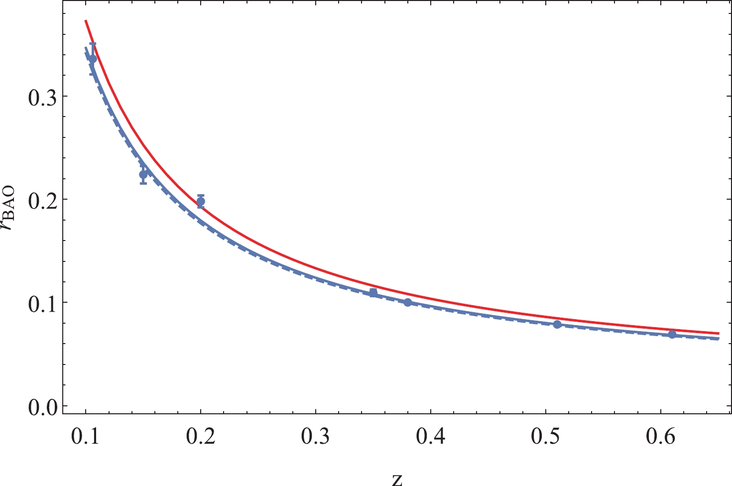
Figure 7. (color online)
$ r_{\rm BAO} $ versus redshift plots in comparison with observational data. Plot of quintom ($ \Lambda $ CDM) model is represented by the solid (dashed) line, and that of Quintom I (II) is in red (blue)In summary, the benchmark model Quintom I yields an equally good fit for the SN Ia data, an acceptable fit for
$ r_{\rm BAO} $ , but a slightly small value of$ \ell_{A} = 285.54 $ . Although the coupled quintom model resolves the Hubble tension, it is in disagreement with the acoustic peak and BAO measurements. However, the complete scan of the parameter space$ (\delta,\Omega_{m}^{(0)}) $ of the coupled quintom model shown in Fig. 8 reveals that there are regions that yield more satisfactory fits to the BAO data and the CMB's first acoustic peak, while significantly alleviating the tension in$ H_{0} $ even though it is not completely resolved. Using the minimization of chi-square for BAO fitting as the anchor, the benchmark quintom model, Quintom II, is defined with$ \lambda_{\phi} = 0.10, \delta = 0.06, \Omega_{m}^{(0)} = 0.308 $ . Quintom II fits the SN Ia data with$ \chi^{2}_{\rm{quin}} = 1026.81 $ for$ M = -19.3925 $ for all 1048 data points. All chi-square values of Quintom II are actually smaller than those of the$ \Lambda $ CDM, as will be shown below.
Figure 8. (color online)
$\chi^{2}$ contours of the quintom model ($\lambda_{\phi}=0.10$ ). Dashed lines represent$\chi^{2}_{l_{1}}$ of the first acoustic peak$l_{1}$ of the CMB spectrum; non-shaded solid lines represent$H_{0}$ of the quintom model.In addition to Quintom II, Fig. 8 shows that the models in the middle region of the parameter space,
$ \delta = 0.02-0.08 $ , can effectively fit both the BAO data and the first CMB peak, while giving the present-time Hubble parameter in the range$ H_{0} = 68-69.5 \; {\rm{km s}}^{-1}{\rm{Mpc}}^{-1} $ . Fig. 9 shows the chi-square contours of the SN Ia fit of the quintom model. The model prefers$ \Omega_{m}^{(0)}\simeq 0.30-0.31 $ for$ \delta = 0-0.10 $ .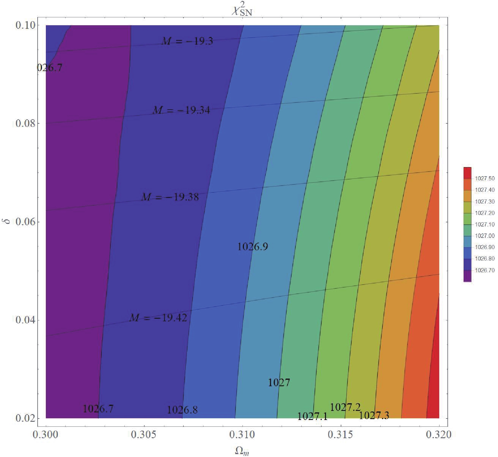
Figure 9. (color online)
$\chi^{2}$ contours of the quintom model ($\lambda_{\phi}=0.10$ ) fitting to the SNIa data. Best-fit M contours are depicted as horizontal lines.To identify the best model, we have to consider the total chi-square of each model. The total chi-square is defined as
$ \chi^2 = \chi^2_{\rm SN} + \chi^2_{\rm BAO} + \chi^2_{l_1} \,, $

(56) where the chi-square of the BAO is given by
$ \chi^2_{\rm BAO} = \sum_{i = 1}^{N_{\rm BAO}} \frac{(r_{\rm BAO\,i,th} - r_{\rm BAO\,i,obs})^2}{\sigma_{r_{\rm BAO\,i}}^2} \,. $

(57) The
$ r_{\rm BAO\,i,th} $ term is defined by Eq. (54), whereas$ r_{\rm BAO\,i,obs} $ and$ \sigma_{r_{\rm BAO\,i}} $ are observational data and error bars as shown in Fig. 7. For the CMB, we consider only the first acoustic peak of the CMB anisotropy, and the chi-square of the first peak is [61]$ \chi^2_{l_1} = \left(\frac{l_{1}^{\rm th} - l_{1}^{ \rm obs}}{\sigma_{l}}\right)^2 \,. $

(58) $ l_{1} $ is the position of the first peak given by [62, 63]$ l_1 = l_A (1 - \delta_1) \,, $

(59) where
$ \delta_1 = 0.267 (r/0.3)^{0.1} $ and$ r = \rho_{r} / \rho_{m} $ at$ z_{\rm dec} $ . From Ref. [64], the first peak of the TT power spectrum is$ l_{1}^{\rm obs} = 220.0 $ , where$ \sigma_{l} = 0.5 $ . We thus find$ \begin{aligned}[b] l_1 (\rm Quintom\; I) =& 210.093 \,, \\ l_1 (\rm Quintom\; II) =& 220.357 \,, \quad l_1 (\Lambda \rm CDM) =& 221.757 \,. \end{aligned} $

The values of chi-square of both models are presented in Table 3.
$ H_{0}/({\rm{km s}}^{-1}{\rm{Mpc}}^{-1}) $ 

$ \chi^2_{\rm SN} $ 

$ \chi^2_{\rm BAO} $ 

$ \chi^2_{l_1} $ 

$ \chi^2 $ 

Quintom I ( $ \delta=0.113 $ )

73.356 1026.74 161.83 392.626 1581.20 Quintom II ( $ \delta=0.06 $ )

68.55 1026.81 13.711 0.5104 1041.03 $ \Lambda $ CDM

67.4 1027.07 21.2862 12.3425 1060.70 Table 3. Chi-square values of the quintom models (
$ \lambda_{\phi} = 0.10 $ ) and the$ \Lambda $ CDM model.Since the quintom model has 2 more parameters (
$ \lambda_{\phi} $ and$ \delta $ ) compared to the$ \Lambda $ CDM model, according to the Akaike Information Criterion (AIC) and the Bayesian Information Criterion (BIC), we must take into account the model's parameters and number of data points as [61]${\rm{AIC}} = \chi _{\rm min}^2 + 2d,$

(60) ${\rm{BIC}} = \chi _{\rm min}^2 + d\ln N,$

(61) where d is the number of the free parameters in the model, N is the number of data points, and
$ \chi^2_{\rm min} $ is the minimum value of the chi-square total. The preferred model is the model that has a small value for AIC and BIC. The$ \Lambda $ CDM model has 4 free parameters ($ \Omega_{m}^{(0)}, \Omega_{b}^{(0)}, H_{0},M $ ), and the data points used in this work are$ 1048 {\rm (SN)} + 7 {\rm (BAO)} + 1 {\rm (CMB)} = 1056 $ . We thus obtain$ \begin{aligned}[b] {\rm AIC \; (Quintom I, II)} =& 1593.20, 1053.03 \,, \\ {\rm AIC \; (\Lambda CDM)} = & 1068.70 \,, \; \\ {\rm BIC \; (Quintom I, II)} =& 1622.97,\; 1082.80 \,, \\ {\rm BIC \; (\Lambda CDM)} =& 1088.55 \,. \end{aligned} $

Comparison of the three observations (the Type Ia supernovae, the baryons acoustic oscillation, and the first acoustic peak of the CMB anisotropy) indicates that the
$ \Lambda $ CDM model is more (less) preferred compared to Quintom I (II). Quintom II alleviates the Hubble tension and even results in better fits to the BAO and CMB$ l_{1} $ data. -
In this work, the Hubble tension is alleviated via the addition of a very small negative density component to the universe. Such a small contribution does not change the values
$ \Omega_{m}^{(0)}\simeq 0.31, \Omega_{DE}^{(0)}\simeq 0.69 $ , which are constrained by the Planck's CMB observations based on the early universe. To realize this idea, we consider a quintom model with conformal phantom-matter coupling and self-interacting quintessence that gives a viable cosmological scenario with the correct density parameters. The model satisfies the general phenomenological conditions, i.e., starting with a radiation dominated era and continuing with matter and dark energy dominated era. It also contains the phantom divide crossing and effectively alleviates the Hubble tension, giving$ H_{0} = 73.356\; {\rm km \; s}^{-1}{\rm Mpc}^{-1} $ and$ \Omega_{m}^{(0)} = 0.308, \;\Omega_{\phi}^{(0)} = 0.692,\; \Omega_{\sigma}^{(0)} = -0.00164 $ , as shown in Table 2.Phenomenologically, as discussed in Section II, the required negative density of the extra component X for
$ w_{X} = 1 $ is$ \Omega_{X}^{(0)} = -5.247 \times 10^{-11} $ . This is based on the assumption of the non-coupling of X to normal matter. In our quintom model, the conformal phantom-matter coupling is introduced to control the size of the negative density of the phantom field,$ \sigma $ . In this coupled model, the negative density of the phantom field becomes$ \Omega_{\sigma}^{(0)} = -0.00164 $ for$ w_{\sigma} = 1 $ .For the benchmark quintom model that mimicked the late-time densities of the
$ \Lambda $ CDM, the small redshift ($ z<10 $ ) iSW effect originated from the dark energy should be closely similar to that of the$ \Lambda $ CDM. We found that the SN Ia fits of the benchmark quintom were just as good as the fiducial$ \Lambda $ CDM but with a different best-fit absolute magnitude M. More precise determination of the absolute magnitude of SN Ia in future observations could potentially identify the superior model. The BAO distance fit with the observation is acceptable, but the$ \Lambda $ CDM fit is better, except for one point ($ z = 0.20 $ ). However, the acoustic peak multipole$ \ell_{A} = 285.54 $ is approximately 5% smaller than that of the observation. The benchmark model Quintom I completely resolves the tension in the Hubble parameter but is in obvious tension with the peak position of the CMB and the BAO measurements. A parameter scan of the quintom model revealed the region$ 0.02<\delta<0.10, \Omega_{m}^{(0)}<0.31 $ of the parameter space, which yielded good to excellent fits for the BAO, first acoustic peak of CMB anisotropy, and SN Ia data. An example of a Quintom II model was presented and demonstrated using AIC and BIC, that it is a better-fit model compared to the$ \Lambda $ CDM, and yet, significantly alleviated the Hubble tension. -
We appreciate the very helpful suggestions from D.M. Scolnic on the SN Ia data.
-
From Table A1, fixed point (a) is a kinetic-dominated point. Radiation dominated epoch can be realized by the fixed point (b), (c), (e), or (f) because
$ w_{\rm eff} = 1/3 $ . Fixed point (b) is a standard radiation dominated era, whereas the other points are a mixture of radiation and other components. Point (d) or (h) can possibly be a matter dominated point, wherein both of them also have a dark energy component in the matter dominated epoch. The accelerated expansion era can be realized by point (g) or (h). Fixed point (g) is an accelerating expansion fixed point that arises in the quintessence model, whereas point (h) is a scaling solution (i.e., the ratio of matter and dark energy is not equal to zero at late-time). Fixed point (d) cannot be an accelerating solution because the dark energy density is not negative. -
The autonomous equations can be rewritten as
$\tag{B1} \begin{aligned}[b] \frac{{\rm d}x_1}{{\rm d}N} =& {\cal F}(x_1,x_2,x_3,x_4) \,, \nonumber \quad \frac{{\rm d}x_2}{{\rm d}N} = {\cal G}(x_1,x_2,x_3,x_4) \,, \nonumber \\ \frac{{\rm d}x_3}{{\rm d}N} = &{\cal H}(x_1,x_2,x_3,x_4) \,, \nonumber \quad \frac{{\rm d}x_4}{{\rm d}N} = {\cal I}(x_1,x_2,x_3,x_4) \,. \end{aligned} $

The stability of the fixed points will be investigated using linear perturbation analysis around each fixed point,
$ (x_1^{(c)}, x_2^{(c)}, x_3^{(c)},x_4^{(c)}) $ , by setting$\tag{B2}{x_i}(N) = x_i^{(c)} + \delta {x_i}(N),$

where
$ i = 1,2,3,4 $ . The perturbation equations then take the form$\tag{B3} \frac{\rm d}{{\rm d}N} \begin{pmatrix} \delta x_1 \\ \delta x_2 \\ \delta x_3 \\ \delta x_4 \end{pmatrix} = {\cal M} \begin{pmatrix} \delta x_1 \\ \delta x_2 \\ \delta x_3 \\ \delta x_4 \end{pmatrix} \,, $

where the matrix
$ {\cal M} $ is given by$\tag{B4} {\cal M} = \left.\begin{pmatrix} \dfrac{\partial {\cal F}}{\partial x_1} \dfrac{\partial {\cal F}}{\partial x_2} \dfrac{\partial {\cal F}}{\partial x_3} \dfrac{\partial {\cal F}}{\partial x_4}\\ \dfrac{\partial {\cal G}}{\partial x_1} \dfrac{\partial {\cal G}}{\partial x_2} \dfrac{\partial {\cal G}}{\partial x_3} \dfrac{\partial {\cal G}}{\partial x_4}\\ \dfrac{\partial {\cal H}}{\partial x_1} \dfrac{\partial {\cal H}}{\partial x_2} \dfrac{\partial {\cal H}}{\partial x_3} \dfrac{\partial {\cal H}}{\partial x_4}\\ \dfrac{\partial {\cal I}}{\partial x_1} \dfrac{\partial {\cal I}}{\partial x_2} \dfrac{\partial {\cal I}}{\partial x_3} \dfrac{\partial {\cal I}}{\partial x_4} \end{pmatrix}\right|_{x_1^{(c)},x_2^{(c)},x_3^{(c)},x_4^{(c)}} \,. $

The first order coupled differential equation (B1) has a general solution
$\tag{B5} \delta x_i \propto {\rm e}^{\mu N}\,, $

where
$ \mu $ is an eigenvalue of the matrix$ {\cal M} $ . Thus, if all eigenvalues are negative (or their real parts are negative for complex eigenvalues), the fixed point is stable. If at least one eigenvalue is positive, the fixed point is a saddle point. When all of the eigenvalues are positive, the fixed point is unstable. The components of the matrix$ {\cal M} $ are as follows:$\tag{B6} \begin{aligned}[b] \frac{\partial {\cal F}}{\partial x_1} =& \frac{1}{2}(-3 + 9 x_1^2 - 3x_2^2 - 3x_3^2 + x_4^3) \,, \\ \frac{\partial {\cal F}}{\partial x_2} =& -3x_1 x_2 + \sqrt{6} x_2 \lambda_{\phi} \,, \frac{\partial {\cal F}}{\partial x_3} = -3 x_1 x_3 \,, \\ \frac{\partial {\cal F}}{\partial x_4} =& x_1 x_4 \,, \\ \frac{\partial {\cal G}}{\partial x_1} =& 3x_1 x_2 - \sqrt{\frac{3}{2}} x_2 \lambda_{\phi} \,, \\ \frac{\partial {\cal G}}{\partial x_2} =& \frac{1}{2}(3 + 3x_1^2 - 9 x_2^2 - 3x_3^2 + x_4^2 - \sqrt{6} x_1 \lambda_{\phi}) \,, \\ \frac{\partial {\cal G}}{\partial x_3} =& - 3 x_2 x_3 \,, \frac{\partial {\cal G}}{\partial x_4} = x_2 x_4 \,, \\ \frac{\partial {\cal H}}{\partial x_1} =& x_1 (3x_3 - \sqrt{6} \delta) \,, \frac{\partial {\cal H}}{\partial x_2} = - x_2 (3 x_3 + \sqrt{6} \delta) \,, \\ \frac{\partial {\cal H}}{\partial x_3} =& \frac{1}{2}(-3 + 3x_1^2 -3x_2^2 -9x_3^2 + x_4^2 + 2\sqrt{6} x_3 \delta) \,, \nonumber \\ \frac{\partial {\cal H}}{\partial x_4} =& x_4 (x_3 - \sqrt{6} \delta) \,, \\ \frac{\partial {\cal I}}{\partial x_1} =& 3x_1 x_4 \,, \frac{\partial {\cal I}}{\partial x_2} = -3 x_2 x_4 \,, \frac{\partial {\cal I}}{\partial x_3} = -3 x_3 x_4 \,, \\ \frac{\partial {\cal I}}{\partial x_4} =& \frac{1}{2}(-1 + 3x_1^2 -3x_2^2 -3x_3^2 + 3x_4^2) \,. \end{aligned} $

Resolving Hubble tension with quintom dark energy model
- Received Date: 2020-06-28
- Available Online: 2021-01-15
Abstract: Recent low-redshift observations have yielded the present-time Hubble parameter value


 DownLoad: