Exotic ΩΩ dibaryon states in a molecular picture

The history of multiquarks goes back to the establishment of the quark model (QM) by Gell-Mann [1] and Zweig [2], where tetraquark $qq\bar q\bar q$ and pentaquark $qqqq\bar q$ configurations were proposed outside of the conventional meson and baryon states. In the last seventeen years, there has been great progress regarding the exploration of tetraquark and pentaquark states, with the observations of the so called $XYZ$ and $P_c$ states [3-10].

A dibaryon is another type of multiquark system, composed of two color-singlet baryons, such as the deuteron (a loosely $np$ bound state in the $^3S_1$ channel [11]). In 1964, non-strange dibaryon sextet $D_{IJ}$ (with $IJ =$ 01, 10, 12, 21, 03, and $30$) was proposed by Dyson and Xuong in SU(6) symmetry [12]. The $D_{01}$, $D_{10}$, and $D_{12}$ dibaryons have been identified as the deuteron ground state, the virtual $^1S_0$ isovector state, and an isovector $J^P = 2^+$ state at the $\Delta N$ threshold, respectively [12]. Recently, the $d^* (2380)$ state was confirmed by the WASA detector at COSY [13-16], which was considered to be the $\Delta\Delta$ dibaryon in the $D_{03}$ channel [17-21]. Moreover, the H-dibaryon predicted by Jaffe [22] is still attractive in terms of both experimental and theoretical aspects [23-26]. For more information about dibaryons, one can consult the recent review paper in Ref. [27].

Compared with the $NN$ and H dibaryons, investigation of the $\Omega\Omega$ system has received considerably less research interest. The interaction between two $\Omega$ baryons has not been adequately understood experimentally and theoretically. Nevertheless, one would expect that the $\Omega\Omega$ dibaryon will be stable against the strong interaction, as $\Omega$ is the only stable state in the decuplet 10 baryons [28]. From the properties of $\Omega$, we know that the baryon number of $\Omega\Omega$ is $2$ and the strangeness $S = -6$, which is the most strange dibaryon state. Under the restriction of the Pauli exclusion principle, the total wave function of the $\Omega\Omega$ system should be antisymmetric, which results in the even total spin $S = 0$ or $S = 2$ for the S-wave ($L = 0$) coupling. Thus, the spin-parity quantum number is $J^P = 0^+$ ($^1S_0$) or $2^+$ ($^5S_2$), and there is no isospin for such a system.

To date, the $\Omega\Omega$ dibaryon states have been studied in a quark potential model [29], the chiral SU(3) quark model [30], and lattice QCD simulations [31, 32]. In the quark potential model [29], the authors calculated the effective interaction between two $\Omega$ baryons by including the quark delocalization and color screening. They found that the mass of the scalar $\Omega\Omega$ system was heavier than the $2m_\Omega$ threshold, resulting in a weakly repulsive interaction. This result was supported by the lattice QCD calculation at a pion mass of 390 MeV in Ref. [31], where weakly repulsive interactions were observed for both the $S = 0$ and the $S = 2$ $\Omega\Omega$ systems. In the chiral SU(3) quark model, the structure of the scalar $\Omega\Omega$ dibaryon was studied by solving a resonating group method equation [30]. Their result suggested a deep attraction with the binding energy near 100 MeV. In Ref. [33], the HAL QCD Collaboration investigated the interaction between two $\Omega$ baryons at $m_\pi = 700$ MeV and found that the $\Omega\Omega$ potential has a repulsive core at short distances and an attractive well at intermediate distances. The phase shift obtained from the potential exhibited moderate attraction at low energies. Recently, the HAL QCD Collaboration performed a $(2+1)$-flavor lattice QCD simulation on the $(\Omega\Omega)_{0^+}$ dibaryon at nearly physical pion mass $m_\pi = 146$ MeV [32]. They found an overall attraction for the scalar $\Omega\Omega$ dibaryon with a small binding energy $B_{\Omega\Omega} = 1.6$ MeV. These conflicting results from the phenomenological models and lattice simulations have inspired more theoretical studies on the $\Omega\Omega$ dibaryon systems. In this work, we shall study the $\Omega\Omega$ dibaryons in both the scalar $^1S_0$ and tensor $^5S_2$ channels using the QCD sum rule method.

In the past several decades, the QCD sum rule has been used as a powerful non-perturbative approach to investigate the hadron properties, such as the hadron masses, magnetic moments, and decay widths [34, 35]. To study the dibaryon systems using QCD sum rules, we need to construct the $\Omega\Omega$ interpolating currents using the local Ioffe current for the $\Omega$ baryon [36, 37]

in which $s(x)$ represents the strange quark field, $a, b, c$ are the color indices, $\gamma_\mu$ is the Dirac matrix, $C = i\gamma_2\gamma_0$ is the charge conjugation matrix, and T is the transpose operator. The $\Omega\Omega$ dibaryon interpolating current is then composed in the molecular picture as

With this interpolating current, we consider the two-point correlation function for $\Omega\Omega$ dibaryon:

where $J^{\Omega\Omega}_{\mu\nu}(x)$ is symmetric and can, thus, couple to both the scalar and tensor dibaryon states that we are interested in:

in which $f_0, f_q$, and $f_T$ are the coupling constants, and $\epsilon_{\mu\nu}$ is the polarization tensor coupling to the spin-2 state. In addition to the $\Omega\Omega$ dibaryon, $J^{\Omega\Omega}_{\mu\nu}$ can also couple to the $\Omega-\Omega$ scattering state with the same quantum numbers. In principle, one should consider both the genuine dibaryon and $\Omega-\Omega$ scattering state contributions to the two-point correlation function in Eq. (3) on the hadron side. However, the contribution from the $\Omega-\Omega$ scattering state cannot affect the hadron mass significantly, similar to the result for the tetraquark system [38]. We will not take this effect into account in our analyses.

We use the following projectors to choose different invariant functions from $\Pi_{\mu\nu,\,\rho\sigma}(q^2)$ [39-41]

where

Projectors $P_{0T}$, $P_{0S}$, and $P_{0TS}$ in Eq. (6) can be used to select different invariant functions induced by the trace part (T), traceless symmetric part (S), and their cross term part (TS) from the tensor current, respectively, which all couple to the $J^P = 0^+$ channel with different coupling constants.

At the hadronic level, the invariant structure of correlation function $\Pi(q^2)$ can be expressed as a dispersion relation:

where $b_n$ is an unknown subtraction constant. The spectral function is usually written as a sum over $\delta$ function by inserting intermediate states $|n\rangle$ with the same quantum numbers as the interpolating current:

where we adopt the “narrow resonance” approximation to describe the spectral function, and $m_{X}$ is the mass of the lowest-lying resonance X.

Using the operator product expansion (OPE) method, the correlation functions can also be calculated as functions of various QCD condensates at the quark-gluonic level. These results are equal to the correlation function in Eq. (8) via the quark-hadron duality. After performing the Borel transform to remove the unknown subtraction constants and suppress the continuum contributions, we establish the QCD sum rules regarding the hadron mass:

in which $s_{0}$ is the continuum threshold, and $M_{B}$ is the Borel mass. Then, we can calculate the hadron mass as

in which spectral density $\rho(s)$ is evaluated at the quark-gluonic level as a function of various QCD condensates up to dimension-16, including the quark condensate $\langle \bar ss\rangle$, quark-gluon mixed condensate $\langle g_s\bar s\sigma\cdot Gs\rangle$, and gluon condensate $\langle g_s^2GG\rangle$. We keep the quark condensate and quark-gluon mixed condensate proportional to $m_s$, which will yield important contributions in the OPE series. The expressions of spectral densities are lengthy; thus, we have presented them in the appendix.

We use the following values for various QCD parameters in our numerical analyses [42-49]:

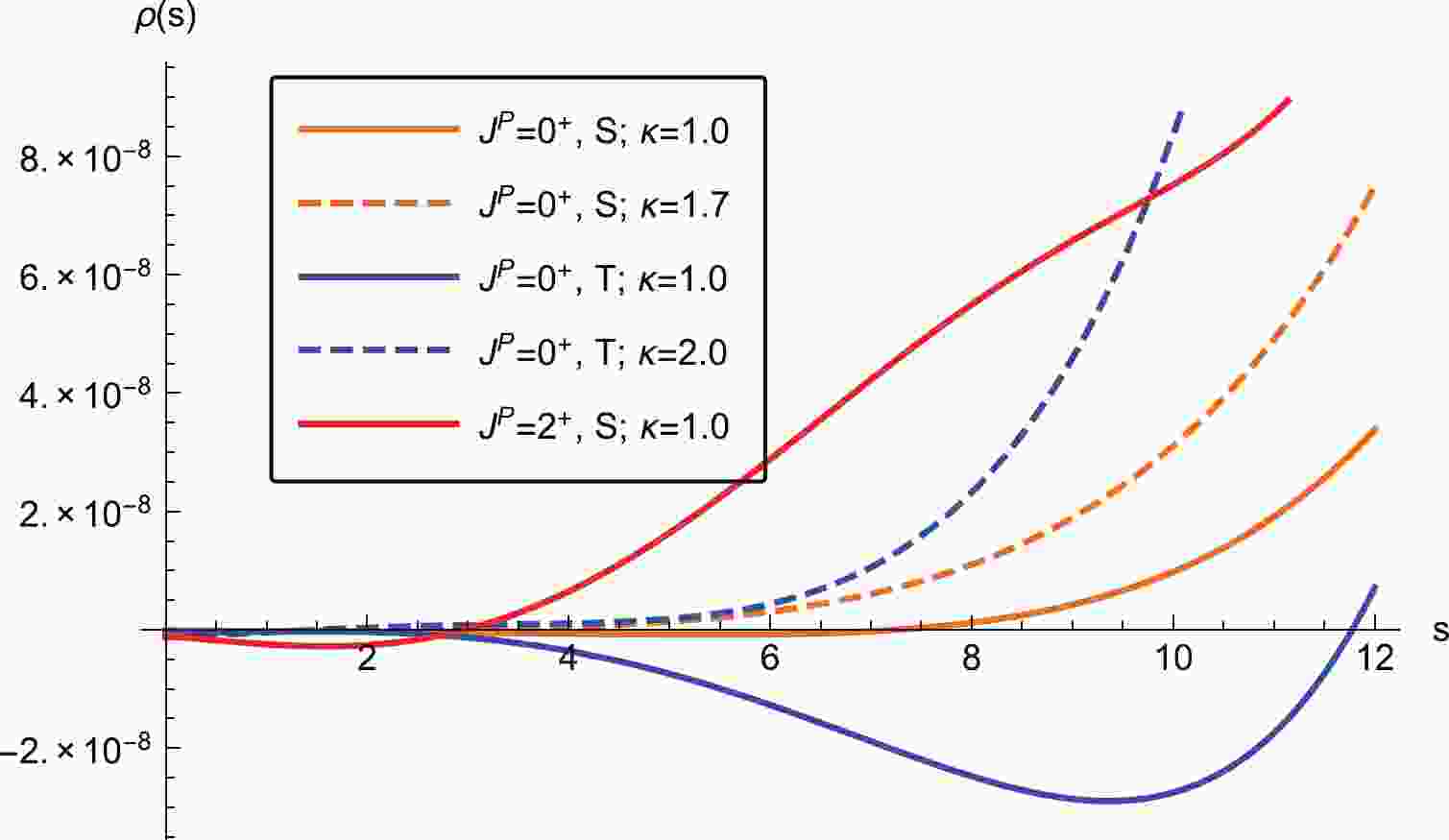
We shall first investigate the trace part (T) of $J^{\Omega\Omega}_{\mu\nu}(x)$ to study the scalar $\Omega\Omega$ dibaryon. Before performing the mass sum rule analysis, we study the behaviors of the spectral densities for the trace part, the traceless symmetric part, and the tensor part. We show these spectral densities in Fig. 1 as three solid lines. It is clear that the spectral density of the trace part for the scalar channel is negative in a broad region of 2 GeV$^2$ $\leqslant s\leqslant 12$ GeV$^2$. This behavior of the spectral density is distinct from those of the traceless symmetric part (S) for the scalar channel and the tensor channel, as shown in Fig. 1. To eliminate this negative effect, we consider the violation of factorization assumption by varying the four-quark condensate $\langle\bar s\bar sss\rangle = \kappa \left< \bar s s \right>^2$ [35]. Because the factorization assumption for the high dimensional condensate ( $D>6$) is not precise and unclear, we shall consider the impact of $\kappa$ if the condensates can be reduced to four-quark condensates, for example, $\langle\bar{s}\bar{s}\bar{s}sss\rangle \to \langle\bar{s}s\rangle\kappa\langle\bar{s}s\rangle^2 = \kappa\langle\bar{s}s\rangle^3$. The numerical values of the gluon condensate and quark-gluon mixed condensate are also provided in Eq. (12). In the case of the $J^P = 0^+$ (T) channel, the factor is naturally taken as $\kappa = 2$. In the case of the $J^P = 0^+$ (S) channel, the behavior of the spectral density is good enough for $\kappa = 1.7$ of the factorization assumption, as shown in Fig. 1. However, we set $\kappa = 1$ for the $J^P = 2^+$ tensor channel because its spectral density is positive in most of the parameter region. To avoid overestimation of the uncertainty of the four-quark condensate, we shall use the fixed value of $\kappa$ and not consider it as an error source for the mass prediction in our following numerical analyses.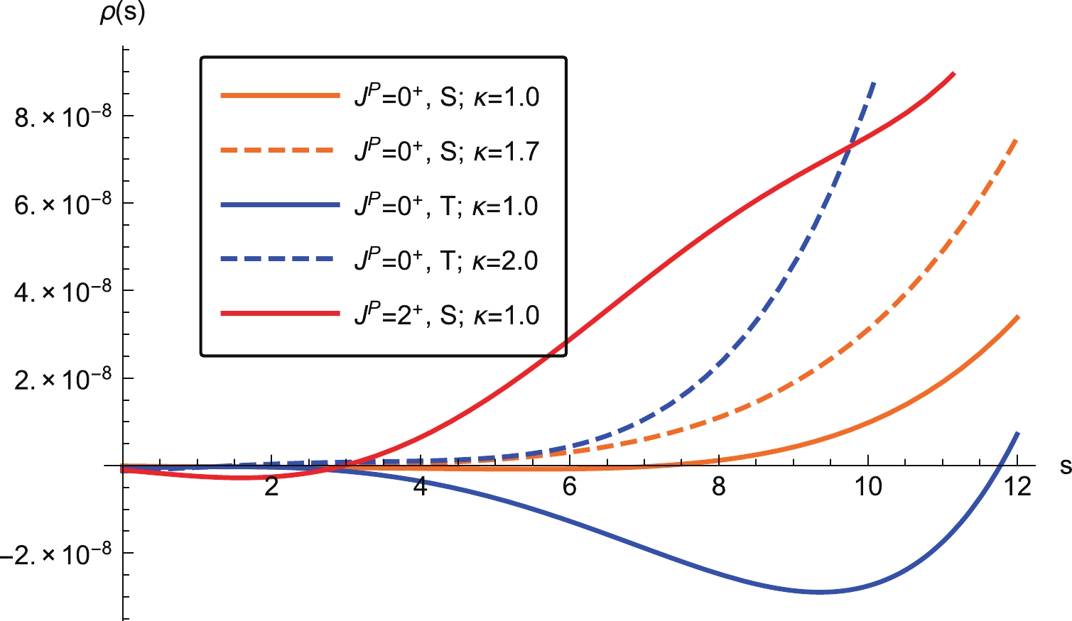

Figure 1.  (color online) Behaviors of the spectral densities for all channels. The solid lines represent the spectral densities for $\kappa=1$, whereas the dashed lines are the corresponding densities considering the effect of factorization assumption.

In Eq. (11), the hadron mass is extracted as a function of two free parameters: the Borel mass, $M_B$, and the continuum threshold, $s_0$. For the numerical analysis, we study the OPE convergence to determine the lower bound on Borel mass $M_B$, requiring the contributions from the dimension-16 condensates to be less than 5%. For the trace part (T) of the scalar channel, we list the two-point correlation function numerically as

in which we take $s_0\to\infty$. According to the above criteria, the lower bound on the Borel mass can be obtained as $M_B^2\geqslant 2.1$ GeV$^2$. Conversely, the upper bound on the Borel mass can be obtained by studying the pole contribution. Requiring the pole contribution to be larger than 10%, we find the upper bound on the Borel mass to be $M_B^2\leqslant 2.9$ GeV$^2$. Finally, the reasonable working region of the Borel mass is 2.1 GeV$^2$ $\leqslant M_B^2\leqslant 2.9$ GeV$^2$.

For continuum threshold $s_0$, an optimized choice is the value minimizing the variation of the hadron mass with the Borel mass. As shown in Fig. 2, we plot the variation of the extracted hadron mass with respect to continuum threshold $s_0$ for the scalar trace part with $J^P = 0^+$ (T). We determine the working region of the continuum threshold to be 13.8 GeV $^2$ $\leqslant s_0\leqslant 14.8$ GeV$^2$.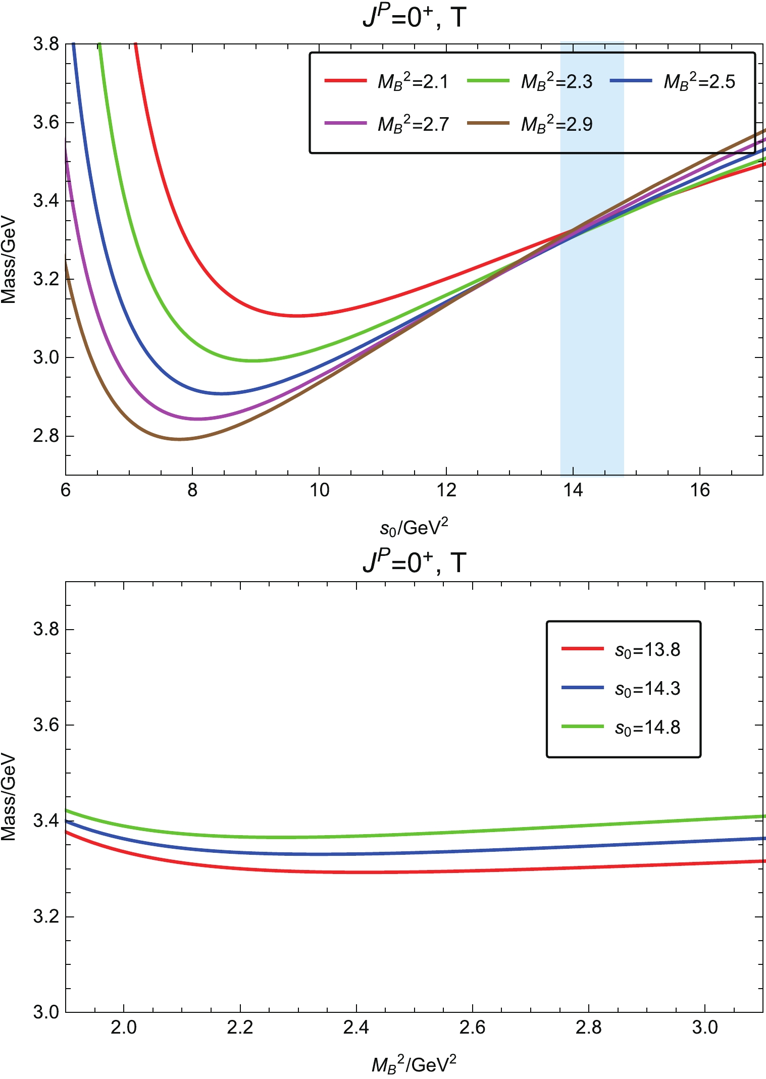

Figure 2.  (color online) Extracted hadron mass for the trace part (T) with $J^P=0^+$.

Within these parameter regions, we plot the Borel curves of the extracted hadron mass in Fig. 2. These Borel curves demonstrate good stability and give the mass prediction of the scalar $\Omega\Omega$ dibaryon with $J^P = 0^+$ (T) as

in which the errors come from the uncertainties of $M_B$, $s_0$, and various QCD parameters in Eq. (12). The corresponding coupling constant can be evaluated as

As indicated in Eq. (6), the traceless symmetric part (S) and cross term (TS) in the tensor correlation function $\Pi_{\mu\nu,\,\rho\sigma}(q^2)$ can also couple to the scalar $\Omega\Omega$ channel with $J^P = 0^+$. A similar analysis is performed for the traceless symmetric part of the scalar channel. The Borel curves are shown in Fig. 3, and the numerical results are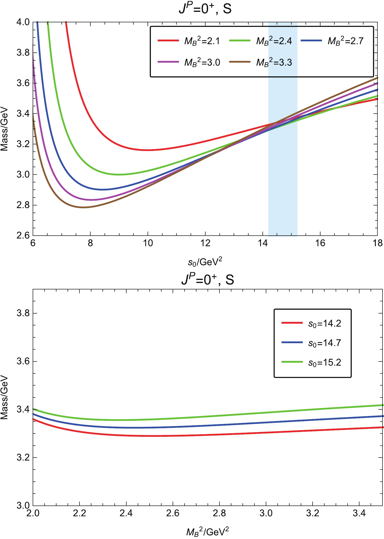

Figure 3.  (color online) Extracted hadron mass for the traceless symmetric part (S) with $J^P=0^+$.

We collect the numerical results for both the trace part and the traceless symmetric part in Table 1. In the case of the cross term (TS), the perturbative term in the OPE series is absent; hence, we will not use this invariant structure to study the scalar dibaryon.

	${\rm{mass}}/{\rm{GeV}}$	${\rm{coupling}}/10^{-4}\,{\rm{GeV}}^8$	pole contribution	$\kappa$	$s_0/{\rm{GeV}}^2$	$M_B^2/{\rm{GeV}}^2$
$(0^+, T)$	$3.33\pm 0.50$	$10.10\pm 5.44$	39%	$2.0$	$[13.8, 14.8]$	$[2.1, 2.9]$
$(0^+, S)$	$3.33\pm 0.52$	$6.25\pm 1.60$	43%	$1.7$	$[14.2, 15.2]$	$[2.1, 3.3]$
$(2^+, S)$	$3.15\pm 0.33$	$9.01\pm 6.60$	20%	$1.0$	$[14.6, 15.6]$	$[2.5, 3.0]$

Table 1.  Numerical results for the trace part (T), traceless symmetric part (S) with $J^P=0^+$, and tensor part with $J^P=2^+$.

Considering both the trace part and the traceless symmetric part, we obtain the mass and coupling constant for the scalar $\Omega\Omega$ dibaryon with $J^P = 0^+$

This obtained hadron mass is approximately 15 MeV below the threshold of $2m_{\Omega}\approx 3345$ MeV [42], suggesting the possibility of the existence of a loosely bound molecular state of the scalar $\Omega\Omega$ dibaryon. The central value of our prediction on the binding energy is in good agreement with the recent HAL QCD result [32], even though it is much smaller than the chiral SU(3) quark model calculation [30].

To investigate the tensor $\Omega\Omega$ dibaryon state, we use projector $P_{2S}^P$ in Eq. (6) to pick out the tensor invariant structure in $\Pi_{\mu\nu,\,\rho\sigma}(q^2)$. Using this invariant function, we perform a similar analysis to that performed for the scalar channels. As emphasized above, we use $\kappa = 1.0$ for the tensor spectral density in our analysis.

We find the parameter working regions to be 2.5 GeV$^2$ $\leqslant M_B^2 \leqslant 3.0$ GeV$^2$ and 14.6 GeV$^2$ $\leqslant s_0\leqslant 15.6$ GeV$^2$ for the Borel mass and continuum threshold, respectively. The mass curves depending on $s_0$ and $M_B^2$ for the tensor channel are accordingly plotted in Fig. 4. Obviously, the mass sum rules are reliable in the above parameter working regions. We obtain the mass for the tensor $\Omega\Omega$ dibaryon with $J^P = 2^+$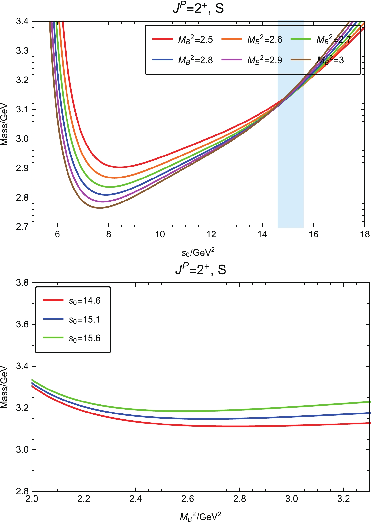

Figure 4.  (color online) Extracted hadron mass for the $J^P=2^+$ tensor channel.

and the coupling constant

The predicted dibaryon mass in Eq. (20) is also below the $2m_\Omega$ threshold, which is even lower than the mass of the scalar $\Omega\Omega$ dibaryon in Eq. (18). This result is different from the weakly repulsive interaction for the tensor $\Omega\Omega$ system obtained by the lattice QCD calculation with a pion mass of 390 MeV in Ref. [31].

In this work, we investigate the scalar and tensor $\Omega\Omega$ dibaryon states in $^1S_0$ and $^5S_2$ channels with $J^P = 0^+$ and $2^+$, respectively, in the framework of QCD sum rules. We construct a tensor $\Omega\Omega$ dibaryon interpolating current in a molecular picture by which the spectral densities and two-point correlation functions are calculated up to dimension sixteen condensates at the leading order of $\alpha_s$.

We use different projectors to pick out spin-0 and spin-2 invariant structures from the tensor correlation function and find that all the trace part (T), traceless symmetric part (S), and cross term (TS) couple to the $0^+$ dibaryon. However, the cross term is not considered for the $0^+$ dibaryon channel because of the absence of the perturbative term in its OPE series. Instead, both the trace part and traceless symmetric part are used to study the mass of the scalar $\Omega\Omega$ dibaryon. Accordingly, we make the reliable mass prediction for the scalar $\Omega\Omega$ dibaryon to be $m_{\Omega\Omega,\, 0^+} = (3.33\pm 0.51)\, {\rm{GeV}}$. This value is not opposed to the existence of a loosely bound scalar $\Omega\Omega$ dibaryon state. Our result supports the attractive interaction existing in the scalar $\Omega\Omega$ channel, with the small binding energy in agreement with the HAL QCD simulation [32]. For the tensor $\Omega\Omega$ system, our result provides a mass prediction near $m_{\Omega\Omega,\, 2^+} = (3.15\pm0.33)\, {\rm{GeV}}$, which is even lower than the scalar channel. Because of the large inherent uncertainty of the QCD sum rule approach, it is not easy to make an accurate prediction for the existence of the $\Omega\Omega$ bound states based on only the above calculations. More investigations using other phenomenological methods are needed in the future to study the masses, decays, and productions for these dibaryon states.

The $\Omega\Omega$ dibaryons, if they do exist, can only decay under the weak interaction because of their small masses. In such molecular systems, an $\Omega$ component in the $\Omega\Omega$ dibaryon can decay as a free particle, while another $\Omega$ acts as the spectator throughout the entire process. Therefore, the dominant decay modes for the scalar $\Omega\Omega$ dibaryon are $\Omega\Omega\to\Omega^-+\Lambda+K^-$, $\Omega\Omega\to\Omega^-+\Xi^0+\pi^-$, and $\Omega\Omega\to \Omega^-+\Xi^-+\pi^0$, whereas only the latter two processes exist for the tensor channel. Moreover, both the scalar and tensor $\Omega\Omega$ dibaryons may decay into the $\Xi\Xi K$ final states. Such exotic strangeness $S = -6$ and doubly-charged $\Omega\Omega$ dibaryon states may be produced and identified in heavy-ion collision experiments in the future, where the strangeness production can be enhanced by the large gluon density.

We thank Prof. Shi-Lin Zhu for useful discussions.

We calculate the spectral densities for the trace part (T), traceless symmetric part (S), cross term part (TS), and tensor part up to dimension-16 condensates and collect all of them as follows:

● For the trace part ($J^P = 0^+$, T),

● For the traceless symmetric part ($J^P = 0^+$, S),

● For the cross term part ($J^P = 0^+$, TS),

● For the tensor part ($J^P = 2^+$, S),