Bayesian inference on isospin splitting of nucleon effective mass from giant resonances in ²⁰⁸Pb

I. INTRODUCTION

• I. INTRODUCTION
• II. MODEL AND METHOD
•      A Nucleon effective mass in Skyrme energy density functional
•      B Nuclear giant resonances
•      C Bayesian analysis
• III. RESULTS AND DISCUSSIONS
• IV. CONCLUSIONS

The nucleon effective mass, which characterizes the momentum or energy dependence of a single nucleon potential in a nuclear medium, is crucial in nuclear physics and astrophysics [1-5]. While various types of nucleon effective masses have been defined in nonrelativistic and relativistic approaches [2-7], in this study, we focus on the total effective mass normally used in the nonrelativistic approach. In asymmetric nuclear matter, effective masses of neutrons and protons, i.e., $m_n^{\ast}$ and $m_p^{\ast}$, respectively, may be different owing to the momentum dependence of the symmetry potential. The difference $m_{n-p}^{\ast}\equiv m_{n}^{\ast}-m_p^{\ast}$ is the so-called isospin splitting of nucleon effective mass, which plays an important role in many physical phenomena and questions in nuclear physics, astrophysics, and cosmology [4, 5]. For example, $m_{n-p}^{\ast}$ affects the isospin dynamics in heavy-ion collisions [8-15], thermodynamic properties of asymmetric nuclear matter [16-18], and cooling of neutron stars [19].

Owing to the limited isospin asymmetry in normal nuclei, the accurate determination of $m_{n-p}^{\ast}$ is difficult. Even the sign of $m_{n-p}^{\ast}$ remains a debated issue. For example, $m_{n-p}^{\ast}> 0$ in neutron-rich matter at the nuclear saturation density $\rho_0 \approx 0.16$ fm^-3 is favored by optical model analyses of nucleon-nucleus scattering data [20, 21], Skyrme energy density functional (EDF) [22] and transport model [23] analyses of nuclear giant resonances, Brueckner-Hartree-Fock calculations [24-27], chiral effective theory [28-30], and an analysis of various constraints on the magnitude and density slope of symmetry energy [31]; in contrast, transport model analyses on single and/or double n/p ratio in heavy-ion collisions [32, 33] (see Ref. [34]) and an energy density functional study on nuclear electric dipole polarizability [35] lead to opposite conclusions.

Understanding these contradictive results and eventually determining the isospin splitting of nucleon effective mass require not only the improvement of both theoretical models/calculations and experimental measurements but also more sophisticated analysis approaches to quantifying the model uncertainties based on given experimental measurements. The latter is a quite general issue in nuclear theory: owing to the lack of a well-settled ab initio starting point, a considerable number of effective theories or models have been developed with parameters determined by fitting empirical knowledge or experimental data [36]. Over the past decade, various statistical approaches, e.g., covariance analysis [37, 38], Bayesian analysis [39-46], and bootstrap method [47, 48], were introduced in nuclear physics studies to quantify uncertainties and evaluate correlations of model parameters. Among them, the Bayesian inference method has been accepted as a powerful statistical approach and is extensively used in various areas of nuclear physics. For a recent review on Bayesian analysis and its application to nuclear structure study, please refer to Ref. [46].

In a previous study of ours [22], we extracted the isospin splitting of nucleon effective mass from the isovector giant dipole resonance (IVGDR) and isocalar giant quadrupole resonance (ISGQR) of ²⁰⁸Pb based on random phase approximation (RPA) calculations using a number of representative Skyrme interactions. However, some factors in the analysis, e.g., the choice of Skyrme interactions and the previously assumed linear relations $1/E_{\mathrm{GQR}}^2$-$m_{s,0}^{\ast}$, could affect the conclusions, and the statistical meaning of the obtained uncertainties are therefore unclear. In the present study, within the framework of Skyrme energy density functional theory and random phase approximation approach, we employed the Bayesian inference method to extract the isospin splitting of nucleon effective mass from the electric dipole polarizability [49, 50], the constrained energy in IVGDR [51], and the ISGQR peak energy [52] in ²⁰⁸Pb. The binding energy [53], charge radius [54], constrained energy of isocalar giant monopole resonance (ISGMR) [55], and neutron $3p_{1/2}-3p_{3/2}$ energy splitting [56] of ²⁰⁸Pb were also included in the analysis to guarantee that the energy density functional can always reasonably describe the ground state and collective excitation state of ²⁰⁸Pb. The isoscalar and isovector effective masses and the neutron-proton effective mass splitting at saturation density, together with the symmetry energy at the subsaturation density $\rho^{\ast} = 0.05\; \mathrm{fm}^{-3}$, were extracted from the Bayesian analysis.

The paper is organized as follows. In Sec. II, we introduce the theoretical models and statistical approaches used in this study. In the next section, we present the results for the uncertainties of model parameters, the isospin splitting of nucleon effective mass at $\rho_0$, and the symmetry energy at $\rho^{\ast} = 0.05\; \mathrm{fm}^{-3}$. Finally, we draw conclusions in Sec. IV.

II. MODEL AND METHOD

• I. INTRODUCTION
• II. MODEL AND METHOD
•      A Nucleon effective mass in Skyrme energy density functional
•      B Nuclear giant resonances
•      C Bayesian analysis
• III. RESULTS AND DISCUSSIONS
• IV. CONCLUSIONS

A Nucleon effective mass in Skyrme energy density functional

• I. INTRODUCTION
• II. MODEL AND METHOD
•      A Nucleon effective mass in Skyrme energy density functional
•      B Nuclear giant resonances
•      C Bayesian analysis
• III. RESULTS AND DISCUSSIONS
• IV. CONCLUSIONS

As in Ref. [22], we studied the nucleon effective mass within the standard Skyrme energy density functional based on the conventional Skyrme interaction:

Here, ${{\sigma}}_i$ is the Pauli spin operator, $P_{\sigma} = (1+{{\sigma}}_1\cdot{{\sigma}}_2)/2$ is the spin-exchange operator, ${{k}} = -{\rm i}({{\nabla}}_1-{{\nabla}}_2)/2$ is the relative momentum operator, and ${{k}}^{\prime}$ is the conjugate operator of ${{k}}$ acting on the left.

Within the framework of Skyrme energy density functional, the nine parameters $t_0- t_3$, $x_0- x_3$, and $\alpha$ of the Skyrme interaction can be expressed in terms of nine macroscopic quantities (pseudo-observables): the nuclear saturation density $\rho_0$, the energy per particle of symmetric nuclear matter $E_0(\rho_0)$, the incompressibility $K_0$, the isocalar effective mass $m_{s,0}^*$ at $\rho_0$, the isovector effective mass $m_{v,0}^*$ at $\rho_0$, the gradient coefficient $G_S$, the symmetry-gradient coefficient $G_{V}$, and the magnitude $E_{\mathrm{sym}}(\rho_0)$ and density slope L of the nuclear symmetry energy at $\rho_0$ [57-59]. The detailed analytical expressions can be found in Refs. [57, 58]. Given that these nine macroscopic quantities have clear physical meaning and available empirical ranges, we used them as model parameters in the Bayesian analysis. Consequently, our model has the following 10 parameters:

In terms of the Skyrme parameters $t_0\sim t_3$ and $x_0\sim x_3$, the nucleon effective mass in asymmetric nuclear matter with density $\rho$ and isospin asymmetry $\delta$ can be expressed as [60]

The well-known isocalar and isovector effective masses, i.e., $m_{s}^{\ast}$ and $m_v^{\ast}$, which are respectively defined as the proton (neutron) effective mass in symmetric nuclear matter and pure neutron (proton) matter, are then expressed as [60]

Once given $m_{s}^{\ast}$ and $m_v^{\ast}$, the isospin splitting of nucleon effective mass can be obtained as [61]

with the isospin splitting coefficients $\Delta m^*_{2n-1}(\rho)$ expressed as

In the following, we use $\Delta m_1^{\ast}$ to indicate the linear isospin splitting coefficient at the saturation density $\rho_0$.

B Nuclear giant resonances

• I. INTRODUCTION
• II. MODEL AND METHOD
•      A Nucleon effective mass in Skyrme energy density functional
•      B Nuclear giant resonances
•      C Bayesian analysis
• III. RESULTS AND DISCUSSIONS
• IV. CONCLUSIONS

Nuclear giant resonances are usually studied using the random phase approximation (RPA) approach [62]. For a given excitation operator $\hat{F}_{\rm JM}$, the strength function is calculated as

with $E_{\nu}$ denoting the energy of the RPA excitation state $|\nu\rangle$; the moments $m_k$ of strength function (sum rules) are usually evaluated as follows:

For the ISGMR, IVGDR, and ISGQR studied here, the excitation operators are defined as follows:

where Z, N, and A are proton, neutron, and mass number, respectively; $r_i$ is the nucleon's radial coordinate; $Y_{\text{1M}}(\hat{r_i})$ and $Y_{\text{2M}}(\hat{r_i})$ are the corresponding spherical harmonic functions.

Particularly, in linear response theory, the inverse energy weighted sum rule can also be extracted from the constrained Hartree-Fock (CHF) approach [63, 64]:

where $\vert\lambda\rangle$ is the ground-state for the nuclear system Hamilton $\mathcal{H}$ constrained by the field $\lambda \hat{F}_J$.

The energy of isoscalar giant monopole resonance (GMR), i.e., the breathing mode, is an important probe of the incompressibility in nuclear matter. It can be evaluated according to the constrained approximation [65] as

where the energy weighted sum rule $m_1$ of ISGMR is related to the ground-state rms radius $\langle r^2 \rangle$ by [66]

Therefore, we calculated $E_{\mathrm{GMR}}$ by using the CHF method for computational efficiency.

Concerning the isovector giant dipole resonance, we considered two observables, namely the electric dipole polarizability $\alpha_{\mathrm{D}}$ and the constrained energy $E_{\mathrm{GDR}}\equiv \sqrt{m_1/m_{-1}}$. Note that $\alpha_{\mathrm{D}}$ in ²⁰⁸Pb probes the symmetry energy at approximately $\rho_0/3$ [61] and is therefore sensitive to both the magnitude and density slope of the symmetry energy at saturation density [67]. It is related to the inverse energy-weighted sum rule in the IVGDR through

Meanwhile, the energy weighted sum rule $m_1$ of IVGDR is related to the isovector effective mass at saturation density $m_{v,0}^{\ast}$ via [22, 62]

where $\kappa$ is the well-known Thomas-Reiche-Kuhn sum rule enhancement. One then has approximately

which suggests that $E_{\mathrm{GDR}}$ is negatively correlated with respect to $m_{v,0}^{\ast}$.

It is well known that the excitation energy of isocalar giant quadruple resonance is sensitive to the isoscalar effective mass at saturation density. For example, in the harmonic oscillator model, the ISGQR energy is [52, 66]

with $\hbar \omega_0$ denoting the frequency of the harmonic oscillator. In the present study, we set $E_{\mathrm{GQR}}$ as the peak energy of the response function obtained from RPA calculations. To obtain a continuous response function, the discrete RPA results were smeared out with Lorentzian functions. The width of Lorentzian functions was set to be 3 MeV to reproduce an experimental width of $\sim3$ MeV for ISGQR in ²⁰⁸Pb.

C Bayesian analysis

• I. INTRODUCTION
• II. MODEL AND METHOD
•      A Nucleon effective mass in Skyrme energy density functional
•      B Nuclear giant resonances
•      C Bayesian analysis
• III. RESULTS AND DISCUSSIONS
• IV. CONCLUSIONS

Bayesian analysis has been widely accepted as a powerful statistical approach to quantifying the uncertainties and evaluating the correlations of model parameters as well as making predictions with a certain confidence level according to experimental measurements and empirical knowledge [39-46]. In this study, we employed the MADAI package [68] to conduct Bayesian analysis based on Gaussian process emulators. For further details on this statistical approach, please refer to, e.g., Ref. [40].

According to Bayes' theorem, the posterior probability distribution of model parameters ${{p}}$ (which we are seeking for), with given experimental measurements ${{\mathcal{O}}}^{\mathrm{exp}}$ for a set of observables ${{\mathcal{O}}}$ can be evaluated as

where $\mathcal{M}$ is the given model, $P({{p}})$ is the prior probability of model parameters ${{p}}$ before being confronted with the experimental measurements ${{\mathcal{O}}}^{\mathrm{exp}}$, and $P( \mathcal{M},{{\mathcal{O}}}^{\mathrm{exp}}|{{p}})$ denotes the likelihood or the conditional probability of observing ${{\mathcal{O}}}^{\mathrm{exp}}$with given model $\mathcal{M}$ predictions at ${{p}}$. The posterior univariate distribution of a single model parameter $p_i$ is given by

and the correlated bivariate distribution of two parameters $p_i$ and $p_j$ is given by

From the univariate distribution, the mean value of $p_i$ can be calculated as

The confidence interval of $p_i$ at a confidence level $1-\alpha$ is normally obtained as the interval between the $(50\alpha)^{\text{th}}$ and $(100-50\alpha)^{\text{th}}$ percentile of the posterior univariate distribution. Particularly, the median value $U_{p_i}$ of $p_i$ is defined as the $50^{\mathrm{th}}$ percentile, i.e.,

Concerning the prior distribution, we assumed that the ten parameters are uniformly distributed in the empirical ranges listed in Table 1. It can be concluded from Eq. (20) that the posterior distribution is determined by the combination of the prior distribution and the likelihood function, which depends on the experimental measurement for an observable. Therefore, the prior distribution is critical in the Bayesian analysis and can significantly affect the extracted constraints. Nevertheless, in the present study, owing to the relatively poor knowledge on $m_{s,0}^{\ast}$ and $m_{v,0}^{\ast}$ in the Skyrme EDF, we assumed large prior ranges for $m_{s,0}^{\ast}$ and $m_{v,0}^{\ast}$. Consequently, the constraints on nucleon effective masses were mainly due to the giant resonance observables. Narrowing the prior ranges for all the parameters by 20% slightly reduced the posterior uncertainties of the iospin splitting of nucleon effective mass by a small percentage.

Table 1

Table 1.  Prior ranges of the ten parameters used.

Quantity	lower limit	upper limit
$\rho_0 /\mathrm{fm}^{-3}$	0.155	0.165
$E_0 /\mathrm{MeV}$	−16.5	−15.5
$K_0 /\mathrm{MeV}$	210.0	250.0
$E_{\mathrm{sym} }(\rho_0) /\mathrm{MeV}$	29.0	35.0
$L /\mathrm{MeV}$	20.0	120.0
$G_S /(\mathrm{MeV}\cdot \mathrm{fm}^{5})$	110.0	170.0
$G_V / (\mathrm{MeV}\cdot \mathrm{fm}^{5})$	−70.0	70.0
$W_0 /(\mathrm{MeV}\cdot \mathrm{fm}^{5})$	110.0	140.0
$m_{s,0}^{\ast}/m$	0.7	1.0
$m_{v,0}^{\ast}/m$	0.6	0.9

DownLoad: CSV

Show Table

The likelihood function was set to be the commonly used Gaussian form

where $\mathcal{O}_i({{p}})$ is the model prediction for an observable at given points ${{p}}$, $\mathcal{O}^{\mathrm{exp}}_i$ is the corresponding experimental measurement, and $\sigma_i$ is the uncertainty or the width of likelihood function. For a given parameter set ${{p}}$, we calculated the following seven observables in ²⁰⁸Pb from Hartree-Fock, CHF, and RPA calculations: the electric dipole polarizability $\alpha_{\rm{D}}$ [49, 50], the IVGDR constrained energy $E_{\rm{GDR}}$ [51], the ISGQR peak energy $E_{\mathrm{GQR}}$ [52], the binding energy $E_B$ [53], the charge radius $r_{C}$ [54], the breathing mode energy $E_{\mathrm{GMR}}$ [55], and the neutron $3p_{1/2}-3p_{3/2}$ energy level splitting $\epsilon_{ls}$ [56]. The experimental values for these seven observables together with the assigned uncertainties are listed in Table 2. Regarding $\alpha_{\mathrm{D}}$ and $E_{\mathrm{GMR}}$, $\sigma_i$ were set to be their experimental uncertainties given in Refs. [49] and [55]; for proper determination of $E_B$, $r_C$, $\epsilon_{ls}$, and $E_{\mathrm{GDR}}$, we assigned them artificial $1\sigma$ errors of 0.5 MeV, 0.01 fm, 0.09 MeV, and 0.1 MeV, respectively; concerning the experimental value and uncertainty of $E_{\mathrm{GQR}}$, we used the weighted average of experimental measurements, i.e., $10.9\pm0.1$ MeV, reported in Ref. [52]. Note that decreasing the artificial errors of $E_B$, $r_C$, $\epsilon_{ls}$, and $E_{\mathrm{GDR}}$ by half slightly reduced the posterior uncertainty of $\Delta m_1^*$ by approximately 7% and did not affect the constraint on the symmetry energy at subsaturation density $\rho^* = 0.05\; \mathrm{fm}^{-3}$.

Table 2

Table 2.  Experimental values and uncertainties used for the binding energy $E_B$ [53], charge radius $r_C$ [54], breathing mode energy $E_{\mathrm{GMR}}$ [55], neutron $3p_{1/2}-3p_{3/2}$ energy level splitting $\epsilon_{ls}$ [56], electric dipole polarizability $\alpha_{\mathrm{D}}$ [49, 50], IVGDR constrained energy [51], and ISGQR peak energy [52] in ²⁰⁸Pb.

	value	$\sigma$
$E_B$/MeV	−1363.43	0.5
$r_C$/fm	5.5012	0.01
$E_{\mathrm{GMR}}$/MeV	13.5	0.1
$\epsilon_{ls}$/MeV	0.89	0.09
$\alpha_{\mathrm{D} }/\mathrm{fm}^3$	19.6	0.6
$E_{\mathrm{GDR}}$/MeV	13.46	0.1
$E_{\mathrm{GQR}}$/MeV	10.9	0.1

DownLoad: CSV

Show Table

According to the prior distribution and defined likelihood function, the Markov chain Monte Carlo (MCMC) process using Metropolis-Hastings algorithm was performed to evaluate the posterior distributions of model parameters. For the 10-dimensional parameter space in this study, a great deal of MCMC steps would be needed to extract posterior distributions. Thus, theoretical calculations for all the MCMC steps are infeasible. Instead, in this study, we first sampled a number of parameter sets in the designed parameter space, and trained Gaussian process (GP) emulators [69] using the model predictions with the sampled parameter sets. The obtained GPs provided fast interpolators and were used to evaluate the likelihood function in each MCMC step.

III. RESULTS AND DISCUSSIONS

• I. INTRODUCTION
• II. MODEL AND METHOD
•      A Nucleon effective mass in Skyrme energy density functional
•      B Nuclear giant resonances
•      C Bayesian analysis
• III. RESULTS AND DISCUSSIONS
• IV. CONCLUSIONS

We first generated 2500 parameter sets using the maximin Latin cube sampling method [70]. Twenty-four of them were located near the edge of the allowed parameter space and led to numerical instability in Hartree-Fock (HF) or RPA calculations. Therefore, we discarded these twenty-four parameter sets and used the remaining 2476 parameter sets in HF, CHF, and RPA calculations to obtain the training data for Gaussian emulators.

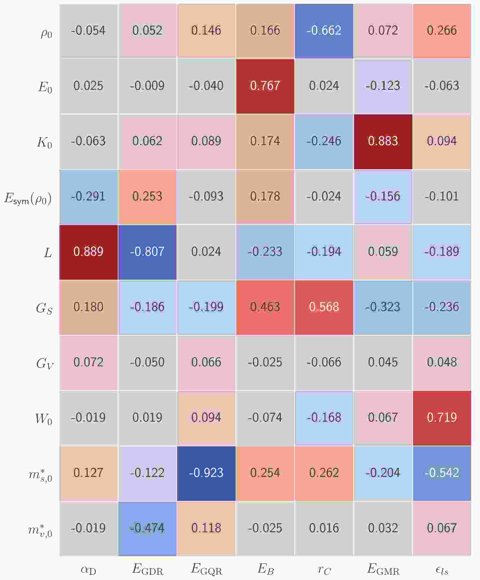
Results from these 2476 training points pointed out possible correlations between observables and model parameters. Fig. 1 shows the Pearson correlation coefficients among model parameters and the seven selected observables obtained from the training data. In Fig. 1, darker red indicates larger positive values, that is, stronger positive correlation, whereas darker blue indicates greater negative values, that is, stronger negative correlation. One can expect that parameters strongly correlated with the chosen observables are more likely to be constrained. Particularly, note that the correlations among observables in nuclear giant resonances and model parameters are clearly consistent with the empirical knowledge introduced in Section II B: $\alpha_{\mathrm{D}}$ is positively (negatively) correlated with L [$E_{\mathrm{sym}}(\rho_0)$] because it is mostly sensitive to the symmetry energy at $\rho^{\ast} = 0.05\; \mathrm{fm}^{-3}$ [61]; $E_{\mathrm{GDR}}$ is negatively correlated with both $m_{v,0}^{\ast}$ and L but positively with $E_{\mathrm{sym}}(\rho_0)$, which can be understood from Eq. (18) and the dependence of $\alpha_{\mathrm{D}}$ on L and $E_{\mathrm{sym}}(\rho_0)$; $E_{\mathrm{GQR}}$ presents a strong negative correlation with $m_{s,0}^{\ast}$ [see Eq. (19)]; $E_{\mathrm{GMR}}$ is mostly sensitive to the incompressibility, denoted as $K_0$. Meanwhile, $G_V$ is weakly correlated with all observables; therefore, it could not be well constrained in the present analysis.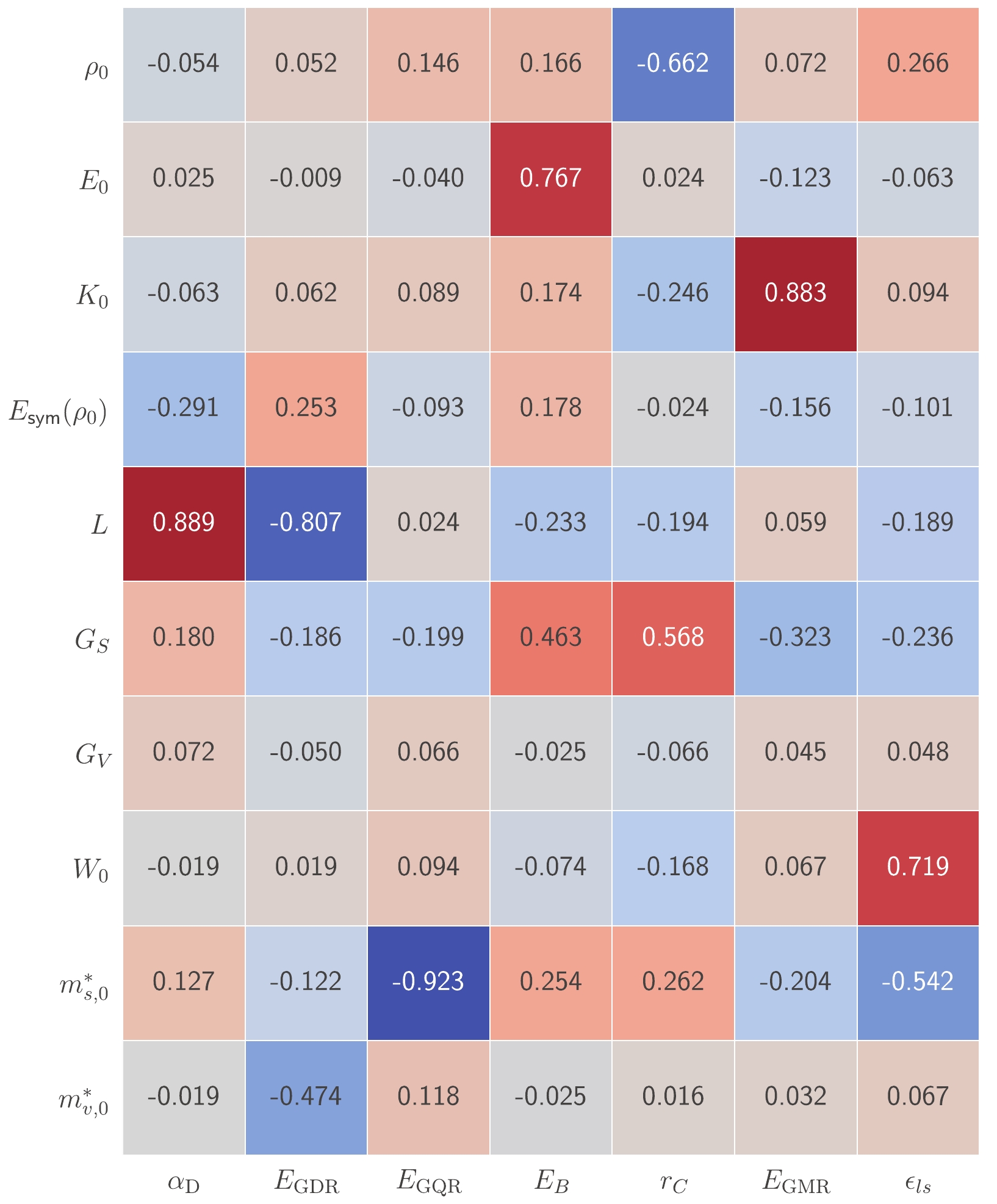

Figure 1

Figure 1.  (color online) Visualization of the Pearson correlation coefficients among model parameters and observables from the training data. The numerical values of correlation coefficients are annotated and color-coded: darker red indicates greater positive values and darker blue indicates greater negative values.

DownLoad: Full-Size Img PowerPoint

Based on the training data, Gaussian process emulators were tuned to quickly predict the model output for the MCMC process. With the help of GPs, we first ran $10^6$ burn-in MCMC steps to allow the chain to reach equilibrium, and then generated $10^7$ points in the parameter space via MCMC sampling. The posterior distributions of model parameters were then extracted from the $10^7$ samples; they are shown in Fig. 2. The lower-left panels show bivariate scatter histograms of the MCMC samples; the diagonal ones present the univariate posterior distribution of the model parameters; the solid, dashed, and dotted lines in the upper-right panels enclose 68.3%, 90%, and 95.4% confidence regions, respectively. Fig. 2 intuitively presents the uncertainties and correlations of the model parameters imposed by the experimental measurements for the chosen observables. Remarkably, $K_0$, $m_{s,0}^{\ast}$, and $m_{v,0}^{\ast}$ are well constrained by the giant monopole, dipole, and quadruple resonances, respectively. Another interesting feature is the strong positive correlation between $E_{\mathrm{sym}}(\rho_0)$ and L, which can be understood by the fact that $\alpha_{\mathrm{D}}$ is positively correlated with L but negatively correlated with $E_{\mathrm{sym}}(\rho_0)$ (see Fig. 1). Similarly, the $E_B$ datum leads to a negative $E_0$-$G_S$ correlation, whereas the $r_C$ datum results in a positive $\rho_0$-$G_S$ correlation. Therefore, the combination of $E_B$ and $r_C$ leads to a negative $\rho_0$-$E_0$ correlation.

Figure 2

Figure 2.  (color online) Univariate and bivariate posterior distributions of the ten model parameters. The solid, dashed, and dotted lines in the upper-right panels enclose 68.3%, 90%, and 95.4% confidence regions, respectively; the diagonal plots show Gaussian kernel density estimations of the posterior marginal distribution for the respective parameters; the lower-left panels show scatter histograms of MCMC samples. The ranges of variations of the ten parameters are the prior ranges listed in Table 1.

DownLoad: Full-Size Img PowerPoint

To quantify the posterior distribution from Bayesian analysis, we listed in Table 3 the statistical quantities estimated from the MCMC samples, including the mean value, median value, and confidence intervals at 68.3%, 90%, and 95.4% confidence levels. The best value, i.e., the parameter set that gives the largest likelihood function, was also listed for reference. In particular, we obtained $m_{s,0}^{\ast}/m =$$0.87_{-0.03}^{+0.02}$ and $m_{v,0}^{\ast}/m = 0.78_{-0.03}^{+0.03}$ at 68% confidence level, and $m_{s,0}^{\ast}/m = 0.87_{-0.04}^{+0.04}$ and $m_{v,0}^{\ast}/m = 0.78_{-0.05}^{+0.06}$ at 90% confidence level. These results are consistent with $m_{s,0}^{\ast} =$$0.91\pm0.05$ and $m_{v,0}^{\ast}/m = 0.8\pm0.03$ extracted from the GDR and GQR in Ref. [22] using the conventional method. Note that, compared with a previous study of ours [22] in which a conventional analysis was carried out based only on 50 representative Skyrme EDFs, in the present study, we extracted the posterior distributions of model parameters from a very large number of parameter sets from MCMC sampling. Therefore, the uncertainties of model parameters were better evaluated, and the constraints obtained in the present study should be more reliable. The 90% confidence interval obtained for $m_{v,0}^{\ast}$ is also in very good agreement with the result of $0.79_{-0.06}^{+0.06}$ from a recent Bayesian analysis of giant dipole resonance in ²⁰⁸Pb [45]. Note that, compared with the present study, the Bayesian analysis in Ref. [45] employed the same GDR data, but the MCMC process was based on fully self-consistent RPA calculations. Therefore, the consistence between the two results further confirms the reliability of Gaussian emulators as a fast surrogate of real model calculations.

Table 3

Table 3.  Best value, mean, median, and confidence intervals of the model parameters from MCMC sampling.

	best	mean	median	68.3% C.I.	90% C.I.	95.4% C.I.
$\rho_0/\text{fm}^{-3}$	0.1597	0.1612	0.1613	$0.1589\sim0.1635$	$0.1577\sim0.1644$	$0.1570\sim0.1647$
$E_0/\text{MeV}$	−16.04	−16.10	−16.10	$-16.34\sim-15.87$	$-16.44\sim-15.78$	$-16.47\sim-15.74$
$K_0/\text{MeV}$	224.6	223.5	223.4	$219.4\sim227.6$	$216.9\sim230.3$	$215.6\sim231.8$
$E_{\text{sym} }(\rho_0)/\text{MeV}$	34.4	32.7	33.0	$30.9\sim34.4$	$29.9\sim34.8$	$29.5\sim34.9$
$L(\rho_0)/\text{MeV}$	48.8	40.3	40.4	$27.9\sim51.9$	$22.8\sim58.1$	$21.4\sim61.1$
$G_S/(\text{MeV}\cdot \text{fm}^5)$	125.7	135.5	135.1	$118.2\sim152.5$	$112.7\sim160.3$	$111.2\sim163.5$
$G_V/ (\text{MeV}\cdot \text{fm}^5)$	65.0	−1.6	−3.1	$-50.9\sim49.5$	$-64.1\sim63.9$	$-67.3\sim67.3$
$W_0/(\text{MeV}\cdot \text{fm}^5)$	111.6	118.4	117.0	$112.0\sim125.1$	$110.6\sim131.4$	$110.3\sim134.7$
$m_{s,0}^*/m$	0.88	0.87	0.87	$0.84\sim0.89$	$0.83\sim0.91$	$0.82\sim0.92$
$m_{v,0}^*/m$	0.78	0.78	0.78	$0.75\sim0.81$	$0.73\sim0.84$	$0.72\sim0.85$

DownLoad: CSV

Show Table

Fig. 3 further shows the posterior bivariate and univariate distributions of the symmetry energy at $\rho^{\ast} = 0.05\; \mathrm{fm}^{-3}$ and the linear isospin splitting coefficient $\Delta m_1^{\ast}$ at $\rho_0$. Given the approximate relations $E_{\mathrm{sym}}(\rho^{\ast}) \propto 1/\alpha_{\mathrm{D}}$ and $E_{\mathrm{GDR}}^2\propto (\alpha_{\mathrm{D}}m_{v,0}^{\ast})^{-1}$, the GDR data lead to positive correlation between $E_{\mathrm{sym}}(\rho^{\ast})$ and $m_{v,0}^{\ast}$. Therefore, Fig. 3 exhibits a negative $E_{\mathrm{sym}}(\rho^{\ast})$-$\Delta m_1$ correlation [see Eq. (7)]. The confidence intervals of $E_{\mathrm{sym}}(\rho^{\ast})$ and $\Delta m^*_{1}$ can be extracted from their univariate distributions shown in Figs. 3(b) and (c). Specifically, we obtained $E_{\mathrm{sym}}(\rho^{\ast}) = 16.7_{-0.8}^{+0.8}\; \mathrm{MeV}$ and $\Delta m_1^{\ast} = 0.20_{-0.09}^{+0.09}$ at 68.3% confidence level, and $E_{\mathrm{sym}}(\rho^{\ast}) = 16.7_{-1.3}^{+1.3}\; \mathrm{MeV}$ and $\Delta m_1^{\ast} = 0.20_{-0.14}^{+0.15}$ at 90% confidence level. For the higher order terms, we found, for example, that $\Delta m_3^{\ast}$ is less than 0.01 at 90% confidence level and therefore can be neglected.

Figure 3

Figure 3.  (color online) Posterior bivariate (a) and univariate [(b) and (c)] distributions of $E_{\mathrm{sym}}(\rho^{\ast})$ at $\rho^{\ast} = 0.05\; \mathrm{fm}^{-3}$, and linear isospin splitting coefficient $\Delta m_1^{\ast}$ at $\rho_0$. The shaded regions in window (a) indicate the 68.3%, 90%, and 95.4% confidence regions.

DownLoad: Full-Size Img PowerPoint

Within the uncertainties, the present constraint on $\Delta m_1^{\ast}$ is consistent with the constraints $m_{n-p}^{\ast}/m = (0.32\pm$$0.15)\delta$ [21] and $m_{n-p}^{\ast}/m = (0.41\pm0.15)\delta$ [20] extracted from a global optical model analysis of nucleon-nucleus scattering data, and also agrees with $\Delta m_1^{\ast} = 0.27$ obtained by analyzing various constraints on the magnitude and density slope of the symmetry energy [31]. It is also consistent with the constraints from analyses of isovector GDR and isocalar GQR with RPA calculations using Skyrme interactions [22] and the transport model using an improved isospin- and momentum-dependent interaction [23]. In addition, the present constraint $E_{\mathrm{sym}}(\rho^*) = 16.7^{+1.3}_{-1.3}$ MeV is consistent with the result $15.91 \pm 0.99$ MeV obtained in Ref. [61], in which the used experimental value of $\alpha_{\mathrm{D}}$ in ²⁰⁸Pb contains a non-negligible amount of contamination caused by quasideuteron excitations [55]. Subtracting the contribution of the quasideuteron effect will slightly enhance $E_{\mathrm{sym}}(\rho^*)$, thereby improving the agreement with the results reported herein .

To end this section, we present the limitations of this study. We only focused on nuclear giant resonances in ²⁰⁸Pb. However, $m_{v,0}^{\ast}$ from the GDR of ²⁰⁸Pb is not consistent with the GDR in ¹⁶O [71]. Describing the giant resonances simultaneously in light and heavy nuclei is still a challenge. Concerning the ambiguities in determining nucleon effective masses from nuclear giant resonances, please refer to Ref. [5]. It is also worth mentioning that owing to the simple quadratic momentum dependence of the single-nucleon potential in Skyrme energy density functional, the nucleon effective mass is momentum independent and only has a simple density dependence [see Eq. (3)], which is not the case in microscopic many body theories, such as the chiral effective theory [29, 30]. The extended Skyrme pseudopotential [72-74] with higher order momentum-dependent terms may help to address the issues on isospin splitting of nucleon effective mass.

IV. CONCLUSIONS

• I. INTRODUCTION
• II. MODEL AND METHOD
•      A Nucleon effective mass in Skyrme energy density functional
•      B Nuclear giant resonances
•      C Bayesian analysis
• III. RESULTS AND DISCUSSIONS
• IV. CONCLUSIONS

Within the framework of Skyrme energy density functional and random phase approximation, we conducted Bayesian analysis for data on the ground and collective excitation states of ²⁰⁸Pb to extract information on the nucleon effective mass and its isospin splitting. Our results indicate that the isoscalar effective mass $m^*_{s,0}/m$ exhibits a particularly strong correlation with the peak energy of isocalar giant quadrupole resonance, and the isovector effective mass $m^*_{v,0}/m$ is correlated with the constrained energy of isovector giant dipole resonance. By including the constrained energy of the isoscalar monopole resonance, the peak energy of isocalar giant quadrupole resonance, the electric dipole polarizability, and the constrained energy of the isovector giant dipole resonance in the analysis, we constrained the isocalar and isovector effective masses and the isospin splitting of nucleon effective mass at saturation density as $m_{s,0}^{\ast}/m =$$0.87^{+0.04}_{-0.04}$, $m_{v,0}^{\ast}/m = 0.78^{+0.06}_{-0.05}$, and $m_{n-p}^{\ast}/m = (0.20_{-0.14}^{+0.15})\delta$, respectively, at 90% confidence level. For a 68.3% ($1\sigma$) confidence level, the constraints become $m^*_{s,0}/m =$$0.87^{+0.02}_{-0.03}$, $m^*_{v,0}/m = 0.78^{+0.03}_{-0.03}$, and $m_{n-p}^{\ast}/m =$$(0.20_{-0.08}^{+0.09})\delta$. In addition, the symmetry energy at the subsaturation density $\rho^{\ast} = 0.05\; \mathrm{fm}^{-3}$ was constrained as $E_{\mathrm{sym}}(\rho^{\ast}) =$$16.7_{-0.8}^{+0.8}\; \mathrm{MeV}$ at 68.3% confidence level and $E_{\mathrm{sym}}(\rho^{\ast}) =$$16.7_{-1.3}^{+1.3}\; \mathrm{MeV}$ at 90% confidence level.

References