Research on the phase space of three- and four-body final states processes

The internal structure and interaction mechanism of microscopic particles is one of the main issues in the field of particle physics. However, due to the extremely short reaction time, the intermediate states of reaction processes can not be measured directly so far. Nevertheless, the distributions of final states, which can reflect the internal structure as well as the interaction mechanism, are measurable. Through these distributions, physicists are able to explore the nature of the various particles and their internal structures. For instance, in 1911, Ernest Rutherford revealed the internal structure of the atom by analyzing the angular distribution of outgoing particles in the well-known gold foil experiment. Therefore, the differential cross-section and the differential decay width play an important role in studying particle physics.

From the Review of Particle Physics (RPP) [1], the differential cross-section for the $2\to n$ scattering process and the differential decay width of a particle into n bodies can be written as follows, respectively:

where $q_i$ and $m_i(i=1,2)$ are the four-momentum and mass of i-th initial particle in the scattering process, respectively, and m is the mass of the parent particle in the decay process. ${\cal{M}}$, which depends on the dynamic mechanisms, is the Lorentz invariant amplitude and ${\rm{d}}\Phi_n$ named as phase space is a purely kinematic factor which is conventionally defined in the following Lorentz-invariant form:

where P is the summation of the four-momenta of all initial states, and $p_i=(E_i, {\boldsymbol{p}}_i)$ is the four-momentum of the i-th particle in the final states. The phase space makes a bridge between the theoretical calculation for ${\cal{M}}$ and the experimental observation for ${\rm{d}}\sigma$ or ${\rm{d}}\Gamma$. The computation of the phase space is of great significance for experimental physicists to analyze distribution data and extract theoretical variables.

One of the most important tasks for particle physicists is to extract the resonance from the invariant mass spectrum of the final states. Generally, besides the invariant amplitude ${\cal{M}}$, the phase space factor also plays an important role in ${\rm{d}}\sigma$ and ${\rm{d}}\Gamma$ in the invariant mass spectrum. Therefore, it is necessary to express the phase space factor in terms of the various invariant mass variables. For example, in the chapter of Kinematics in the RPP, the three-body phase space is expressed in two forms. One contains one invariant mass variable and the other two independent invariant masses which can be visualized by the well-known Dalitz plot. There have been some work on the phase space of n-body final states with $n>3$. Some systematic methods have been introduced in textbooks and articles, for example, Refs. [2–6]. All of these works provide various formulas to calculate three-, four- and n-body phase space distributions and integrations. Recently, in Ref. [7], a new systematic graphic method to decompose an arbitrary n-body phase space has been introduced.

On the experimental side, more and more new particles have been discovered from three- and four-body final states. If the invariant mass variables are properly chosen, the resonance can be extracted much more efficiently. Otherwise, the signal is not obvious and sometimes may even be buried in the background. Therefore, in this paper, we focus on the three- and four-body final states and present the expressions of ${\rm{d}}\Phi_3$ and ${\rm{d}}\Phi_4$ directly in terms of all possible sets of invariant mass variables, using a new formulation, which can serve as a handbook which may be convenient as well as helpful for experimental data analysis.

For n-body final states, there are $3n$ kinematic variables but only $3n-4$ of these are independent because of the law of energy–momentum conservation. Therefore, there are 8 independent kinematic variables (IKVs) for four-body final states. Particularly, if the system is rotation-invariant, such as a decay process of a non-polarized parent particle, three kinematic variables describing the absolute direction of the three-momenta of the final particles can be trivially integrated out. Even so, there are still 5 IKVs for four-body final states. In this paper, all cases for choosing IKVs within invariant mass variables are listed. Then the phase space factor is calculated for each case and furthermore, the four-momenta of the four final states are expressed as functions of IKVs. Once this is complete, the amplitude ${\cal{M}}$ of any interaction mechanism can be expressed quite straightforwardly.

This paper is organized as follows. After the introduction, the notation of this paper is defined in Section II. In Sections III and IV, formulae of the phase spaces of three- and four-body final states are enumerated, respectively. Then by using the formulae given in Section III, two possible mechanisms are distinguished for the reaction $e + p\to e+J/\psi+p$ at the Electron–Ion collider at China (EicC), which will be helpful to search $P_c$ resonance states. The related results are shown in Section V. Furthermore, we also give an example of a four-body case in Section VI. Finally, a brief summary is given in Section VII.

In this section, the notation used in this paper is introduced. The main task of this paper is to present all possible phase space factors in terms of different IKVs for three- and four-body final states. The key problem is how to find all sets of IKVs. In principle, IKVs can be divided into two parts: angular variables and the others which can be expressed as functions of several invariant mass variables, such as energies of particles. As discussed above, since the invariant mass spectrum plays an important role in extracting resonances, invariant mass and angular variables are chosen as the IKVs in this paper for further application.

There are two rules which are useful for classifying different sets of IKVs. Firstly, the number of invariant mass variables appearing in the set of IKVs is counted for the preliminary classification. For example, in the three-body final states, there are only three cases: two, one, and zero invariant mass variables in the set of IKVs. Secondly, we consider the different patterns of the set of IKVs but do not distinguish the order of particles. For example, if only two invariant mass variables are in the set of IKVs for the three-body final states, there are three choices as $(m_{12},\,m_{13})$, $(m_{12},\,m_{23})$, and $(m_{23},\,m_{13})$, which are all equivalent. By following the above two rules, there are only three different sets of IKVs in the three-body final states as shown in the next section. However, with regard to the four-body system, it is much more complicated and a new concept of distribution number (DN) will be introduced in detail in Section IV.

On the other hand, all the angular variables can be distinguished in three classes: three Euler angles for the whole reaction system, the polar angles in the sub-system, and various angles between the three-momenta of a certain two particles. Firstly, Euler angles $\alpha,\beta,\gamma$ describe the absolute direction in the fixed frame $Op_xp_yp_z$ or equivalently $Oxyz$. Euler angles here are defined in the y-convention. Assuming that at the beginning, the direction of ${\boldsymbol{p}}_{\bf{1}}$ is along ${{\boldsymbol{e_z}}}$ and ${\boldsymbol{p}}_{\bf{2}}$ lies in the $p_zOp_x$ plane with ${\boldsymbol{p}}_{\bf{2}}\cdot{{\boldsymbol{e_x}}}>0$ and rotating the configuration of momenta around the axis of ${{\boldsymbol{e_z}}}$, ${{\boldsymbol{e_y}}}$ and ${\boldsymbol{p}}_{\bf{1}}$ in succession by α, β and γ respectively, one can obtain the direction of the momenta of the final states. The overall effect of the successive rotations defined above can be described by the matrix as

Secondly, when it comes to the rest frame of the composite particle $i_1i_2...i_m$ with three-momentum ${\boldsymbol{p}}={\boldsymbol{p}}_{{\boldsymbol{i}}_{\bf{1}}}+{\boldsymbol{p}}_{{\boldsymbol{i}}_{\bf{2}}}+ ... +{\boldsymbol{p_{i_m}}}$, its coordinate axes $O p_x^\star p_y^\star p_z^\star$ are built according to the following procedure. Firstly, the $p_z^\star$ axis is chosen to be along the opposite direction to ${\boldsymbol{p}}$. Secondly, the $p_y^\star$ axis is defined by ${\boldsymbol{e}}_y^\star = {\boldsymbol{e}}_z \times {\boldsymbol{e}}_z^\star$. Thirdly, the $p_x^\star$ axis is naturally determined since $Op_x^\star p_y^\star p_z^\star$ is right-handed. Then, the polar angle of the particle in the coordinates $O p_x^\star p_y^\star p_z^\star$ in this paper can be defined unambiguously.

After all IKVs are fixed, the phase space can be expressed as

where $(m_a,\,m_b,\,\cdots)$ and $(\alpha_1, \,\alpha_2 ,\,\cdots)$ indicate invariant mass and angular variables, respectively. The value of A, which is the phase space factor with the $(m_a,\,m_b,\,\cdots, \, \alpha_1, \alpha_2 ,\,\cdots)$, needs to be derived. Writing down the amplitude ${\cal{M}}$ as a function of IKVs is also helpful. Since ${\cal{M}}$ is actually a function of the three-momenta of final states, it can be obtained quite straightforwardly once the three-momenta can be expressed exactly in terms of IKVs. Therefore, another task of this paper is to provide explicit formulae with the IKVs. Such expressions can be quite complicated, so several intermediate variables will be used for the sake of simplification.

In summary, all cases of IKVs with the invariant mass and angular variables for three- and four-body systems will be listed. Not only the phase space factor A defined in Eq. (5) but also the explicit expressions of the three-momenta of final states are to be given.

There are three distinct sets of IKVs for three-body final states, which contain two, one, and zero invariant mass variables, respectively. In Tables 1–3, the IKVs, the phase space factor A defined in Eq. (5) and the three-momenta of the final states are listed for these three sets. The three-momentum of the third particle can be obtained by $-{\boldsymbol{p}}_1-{\boldsymbol{p}}_2$ and hence will not be shown in the tables. For the last set, shown in Table 3, there are no invariant mass variables and $\theta_{ij}$ is the angle between the three-momenta of the i-th and the j-th particles. Furthermore, ${\left| {{\boldsymbol{p_i}}} \right|}$ satisfies an equation as shown in the last row of Table 3. Though the analytical solution exists, the explicit expression is so complicated that we will not show it there.

IKVs	$m_{13}^2,m_{23}^2,\alpha,\cos\beta,\gamma$
A	$\dfrac{1}{8\left(2\pi\right)^9 4 m^2}$
${\boldsymbol{p}}_{\bf{1,\,2}}$	$\left( \begin{array}{*{20}{c}}{p_{1x}}\\{p_{1y}}\\{p_{1z}}\end{array} \right) = {\cal{R}} \left( {\begin{array}{*{20}{c}}0\\0\\{\left| {{{\boldsymbol{p}}_{\bf{1}}}} \right|}\end{array}} \right), \left( \begin{array}{l}{p_{2x}}\\{p_{2y}}\\{p_{2z}}\end{array} \right) = {\cal{R}} \left( {\begin{array}{*{20}{c}}{\left| {{{\boldsymbol{p}}_{\bf{2}}}} \right|\sin \theta }\\0\\{\left| {{{\boldsymbol{p}}_{\bf{2}}}} \right|\cos \theta }\end{array}} \right)$
	$\begin{array}{l} \;\;\left|{\boldsymbol{p}}_{\bf{1}}\right| =\dfrac{\lambda^{\frac{1}{2}}\left(m^{2}, m_{1}^{2}, m_{23}^{2}\right)}{2 m} \\ \;\; \left|{\boldsymbol{p}}_{\bf{2}}\right| =\dfrac{\lambda^{\frac{1}{2}}\left(m^{2}, m_{2}^{2}, m_{13}^{2}\right)}{2 m} \\ \cos \theta =\dfrac{2 E_{1} E_{2}-\left(m^{2}+m_{3}^{2}-m_{13}^{2}-m_{23}^{2}\right)}{2\left|{\boldsymbol{p}}_{\bf{1}}\right|\left|{\boldsymbol{p}}_{\bf{2}}\right|} \end{array}$

Table 1.  Set of IKVs containing two invariant mass variables. A is the phase space factor and here ${\rm{d}}\Phi_3 =$$A {\rm{d}} m_{13}^2 {\rm{d}} m_{23}^2 {\rm{d}}\alpha {\rm{d}}(\cos\beta) {\rm{d}}\gamma$ which is consistent with Eq. (5). In the last row, expressions for some intermediate variables defined to simplify the expressions of the three-momenta are given. The Källén triangle function $\lambda(x,y,z)$ is applied here as $\lambda(a^2,b^2,c^2)=(a^2-(b+c)^2)(a^2-(b-c)^2)$. The distribution under these IKVs is known as the Dalitz plot and its domain is given in the Kinematics chapter of Review of Particle Physics (RPP) [1].

IKVs	α, cosβ, γ, θ12, θ13
A	$\dfrac{\left|{\boldsymbol{p}}_{\bf{1}}\right|^{2}\left|{\boldsymbol{p}}_{\bf{2}}\right|^{2} \sin ^{2} \theta_{12}}{8(2 \pi)^{9}\left(E_{2} E_{3} \sin ^{2} \theta_{13}+E_{1} E_{3} \sin ^{2}\left(\theta_{12}+\theta_{13}\right)+E_{1} E_{2} \sin ^{2} \theta_{12}\right)}$
${\boldsymbol{p}}_{\bf{1,\;2}}$	$\left(\begin{array}{l}p_{1 x} \\ p_{1 y} \\ p_{1 z}\end{array}\right)={\cal{R}}\left(\begin{array}{c}0 \\ 0 \\ \left|{\boldsymbol{p}}_{1}\right|\end{array}\right),\left(\begin{array}{l}p_{2 x} \\ p_{2 y} \\ p_{2 z}\end{array}\right)={\cal{R}}\left(\begin{array}{c}\left|{\boldsymbol{p}}_{\bf{2}}\right| \sin \theta_{12} \\ 0 \\ \left|{\boldsymbol{p}}_{\bf{2}}\right| \cos \theta_{12}\end{array}\right)$
	$\begin{array}{c}\left| { {\boldsymbol{p} }_{\bf{1} } } \right| = \dfrac{\sin\theta_{13} }{\sin\theta_{12} }\left| { {\boldsymbol{p} }_{\bf{3} } } \right|\\\left| { {\boldsymbol{p} }_{\bf{2} } } \right| = -\dfrac{\sin\left(\theta_{12}+\theta_{13}\right)}{\sin\theta_{12} }\left| { {\boldsymbol{p} }_{\bf{3} } } \right|\\ {\rm{where} }\;\sqrt{\left| { {\boldsymbol{p} }_{\bf{1} } } \right|^2 + m_1^2} + \sqrt{\left| { {\boldsymbol{p} }_{\bf{2} } } \right|^2+m_2^2} + \sqrt{\left| { {\boldsymbol{p} }_{\bf{3} } } \right|^2 + m_3^2} = m\end{array}$

Table 3.  Set of IKVs not containing any invariant mass variables. A is the phase space factor and here ${\rm{d}}\Phi_3 = A {\rm{d}}\alpha{\rm{d}}(\cos\beta){\rm{d}}\gamma{\rm{d}}\theta_{12}{\rm{d}}\theta_{23}$ which is consistent with Eq. (5). The domain of the IKVs is $0 \le \alpha\le2\pi$, $-1\le\cos\beta\le1$, $0\le\gamma\le2\pi$, $0\le\theta_{12}\le\pi$, and $\pi - \theta_{12}\le\theta_{13}\le\pi$.

IKVs	$m_{12},\Omega_3=(\cos\theta_3,\phi_3),\Omega_1^\star=(\cos\theta_1^\star,\phi_1^\star)$
A	$\frac{\left|{\boldsymbol{p}_{\bf 1}^{\bf\star} } \right|\left|{ {\boldsymbol{p} }_{\bf{3} } }\right|}{\left(2\pi\right)^9 8m}$
${\boldsymbol{p}}_{\bf{1,\;2}}$	$\begin{array} {l} p_{1x} =\left|{\boldsymbol{p}_{\bf 1}^{\bf\star} }\right|\left(h\cos\phi_3-\sin\phi_3 k\right) + s_1\sin\theta_3 \cos\phi_3 \\ p_{1y} =\left|{\boldsymbol{p}_{\bf 1}^{\bf\star} }\right|\left(h\sin\phi_3+\cos\phi_3k\right) + s_1\sin\theta_3 \sin\phi_3 \\ p_{1z} =-\left|{\boldsymbol{p}_{\bf 1}^{\bf\star} }\right|\sin\theta_3\sin\theta_1^{\star}\cos\phi_1^{\star} +s_1\cos\theta_3 \\ p_{2x} =\left|{\boldsymbol{p}_{\bf 1}^{\bf\star} }\right|\left(-h\cos\phi_3+\sin\phi_3 k\right) +s_2\sin\theta_3\cos\phi_3 \\ p_{2y} =\left|{\boldsymbol{p}_{\bf 1}^{\bf\star} }\right|\left(-h\sin\phi_3-\cos\phi_3k\right) +s_2 \sin\theta_3\sin\phi_3 \\ p_{2z} =\left|{\boldsymbol{p}_{\bf 1}^{\bf\star} }\right|\sin\theta_3\sin\theta_1^{\star}\cos\phi_1^{\star} +s_2\cos\theta_3 \end{array}$
	$\begin{array}{l} \;\;h =\cos\theta_3\sin\theta_1^{\star}\cos\phi_1^{\star}, \\ \;\;k =\sin\theta_1^{\star}\sin\phi_1^{\star} \\ \;s_1 =-\gamma\beta\sqrt{m_1^2+\left|{\boldsymbol{p}_{\bf 1}^{\bf\star} }\right|^2}+\gamma\left|{\boldsymbol{p}_{\bf 1}^{\bf\star} }\right|\cos\theta_1^{\star} \\ \;s_2 =-\gamma\beta\sqrt{m_2^2+\left|{\boldsymbol{p}_{\bf 1}^{\bf\star} }\right|^2}-\gamma\left|{\boldsymbol{p}_{\bf 1}^{\bf\star} }\right|\cos\theta_1^{\star} \\ \left|{\boldsymbol{p}_{\bf 1}^{\bf\star} }\right| =\frac{\lambda^\frac{1}{2}\left(m^2_{12},m^2_1,m^2_2\right)}{2m_{12} } \\ \left|{ {\boldsymbol{p} }_{\bf{3} } }\right| =\frac{\lambda^\frac{1}{2}\left(m^2,m^2_{12},m^2_3\right)}{2m} \\ \; \gamma\beta =\sqrt{\gamma^2 -1 }=\frac{\left|{ {\boldsymbol{p} }_{\bf{3} } }\right|}{m_{12} } \end{array}$

Table 2.  Set of IKVs containing one invariant mass variable. $\Omega_3=(\cos\theta_3,\phi_3)$ and $\Omega_1^\star=(\cos\theta_1^\star,\phi_1^\star)$ are the solid angles of particle 3 in the rest frame of mass and particle 1 in the rest frame of composite particle 1-2, respectively. A is the phase space factor and here ${\rm{d}}\Phi_3 = A {\rm{d}} m_{12} {\rm{d}} \Omega_3 {\rm{d}}\Omega^\star_1$ which is consistent with Eq. (5). In the last row, expressions for some intermediate parameters defined to simplify the expressions of the three-momenta are given. The domain of the IKVs is $m_1 + m_2 \le m_{12} \le m-m_3$, $-1\le \cos\theta_3,\cos\theta_1^* \le 1$, and $0\le \phi_3,\phi_1^* \le 2\pi$.

For the four-body final states, there are six and four invariant masses variables for systems with two ($m_{ij},i<j$) and three ($m_{ijk},i<j<k$) particles respectively. However, only five of these are independent because of the following five equations,

Therefore, up to 5 invariant masses can be chosen as IKVs.

In principle, there are $\sum_{i=1}^5 C^i_{10} = 462$ ($C^a_b\equiv b!/ (a!(b-a)!)$ is the combination number) different sets of the invariant masses. However, many of them are equivalent. In order to classify all possible unique sets, a new concept of distribution number (DN) denoted by $(n;m;abcd)$ is introduced here. Numbers in the bracket have the following meanings: n denotes the number of invariant masses and obviously satisfies the restriction $0\leq n \leq 5$; abcd denotes the times that the particle index appears in the subscripts with $a\ge b\ge c\ge d$; m denotes the summation $a+b+c+d$. For instance, for the set $\{m_{12}^2, m_{23}^2, m_{123}^2, {\rm{some\;angles}}\}$, $n=3$, $m=7$ and $abcd=3220$. Here $a=3$ for particle index 2 appears three times in the subscripts of three invariant mass variables, and $b=2$, $c=2$ and $d=0$ are for particle 1, 3 and 4, respectively. Because of the restriction of $a\ge b\ge c\ge d$, cases that only differ by the order of the particle indices will correspond to the same DN. For example, the sets $(m_{23}, m_{24}, m_{12}, m_{34}, m_{123})$ and $(m_{12}, m_{13}, m_{14}, m_{23}, m_{124})$ both correspond to DN = (5;11;4322), which means they can be transformed into each other by changing the particle indexes from (1234) to (2341). Therefore, the number of inequivalent sets of the invariant mass reduces from 462 to about 30. Typically, one DN may contains 2 different sets of IKVs. Fortunately, this only happens with DN = (4;9;3321) and (3;7;2221). Furthermore, some cases corresponding to different DNs are of the same kinematic structure because of Eqs. (12) – (16). For instance, if any $m_{ijk}$ is in the set containing five invariant masses, then it can be easily transformed into the set containing five $m_{ij}$ whose DN = (5;10;3322). Table 4 shows such conversions and a representative of each case is picked. In the end, 22 distinct cases survived.

Others	Representative	Example (ij is short for $m_{ij}$)
$(5;m;abcd)$	$(5;11;4322)$	$12,13,14,23,24\rightarrow 12,13,14,23,124$
$(4;9;3222)$	$(4;8;3221)$	$12,13,34,124\rightarrow 12,13,23,34$
$(4;9;3321)$	$(4;10;4321)$	$12,13,23,124\rightarrow 12,13,123,124$
	$(4;8;3221)$	$12,13,24,123\rightarrow 12,13,23,24$
$(4;10;3331)$	$(4;8;3221)$	$12,13,123,234\rightarrow 12,13,14,23$
$(4;11;3332)$	$(4;11;4322)$	$12,124,134,234 \rightarrow 12,124,123,134$
$(3;6;2220)$	$(3;7;3220)$	$12,14,24\rightarrow 12,14,124$
$(3;7;2221)$	$(3;6;3111)$	$12,13,234\rightarrow 12,13,14$
$(3;8;2222)$	$(3;7;2222)$	$12,134,234 \rightarrow 12,34,234$

Table 4.  Cases in the "others" column can be easily transformed into the case in the "Representative" column. There are two distinct cases with DN = (4;9;3321) as well as (3;7;2221), where the particle corresponding to $d=1$ can appear in $m_{ij}$ or $m_{ijk}$.

In our notation, if ${\left| {{\boldsymbol{p_i}}} \right|}$ and $\theta_{ij}$ for each particle are all known, general expressions for components of three-momenta in terms of Euler angles can be calculated as

where ${\cal{R}}$ is defined in Eq. (4), and $A_g$ is defined as

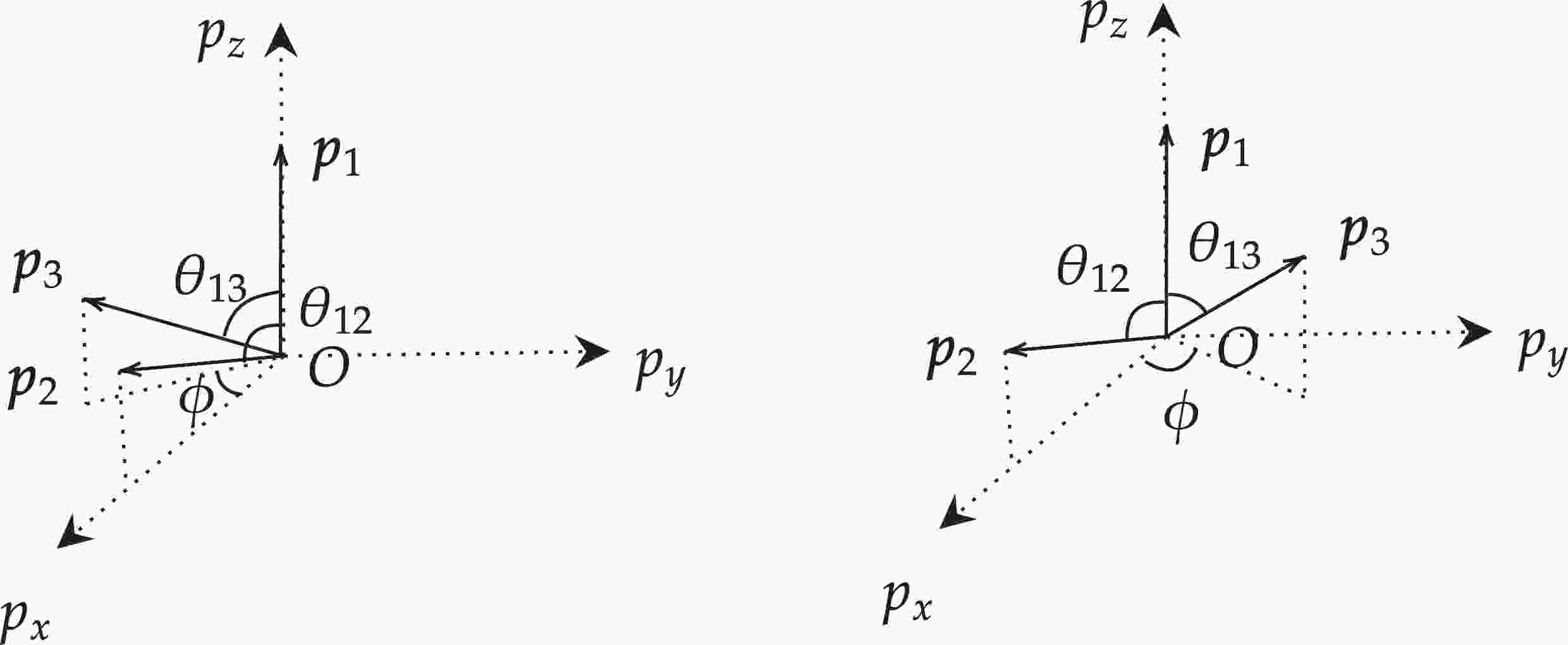
It is clear that we only need six variables, including ${\left| {\boldsymbol{p}}_{\bf{1}} \right|}$, ${\left| {\boldsymbol{p}}_{\bf{2}} \right|}$, ${\left| {\boldsymbol{p}}_{\bf{3}} \right|}$, $\theta_{12}$, $\theta_{23}$ and $\theta_{13}$, to compute all three-momenta of the final states. Note that there are two choices with different sign for $p_{3y}$. These corresponds to the two allowed patterns if just $\theta_{ij}$ and ${\left| {{\boldsymbol{p_i}}} \right|}$ are fixed, as shown in Fig. 1 where Euler angles have been chosen as $(\alpha,\beta,\gamma)= (0,0,0)$. Actually, the two configurations in Fig. 1 are indistinguishable with respect to the IKVs we have chosen. To avoid this arbitrariness, some more variables denoting the sign of $({\boldsymbol{p}}_1\times{\boldsymbol{p}}_2)\cdot{\boldsymbol{p}}_3$ are needed. However, this is unnecessary because the phase space factors A for these two configurations are exactly the same. Thus, one set of IKVs will give at least two sets of three-momenta for the final states, and then the amplitudes of these two three-momenta could be different. We should rewrite Eq. (5) as follows:

Figure 1.  Two patterns are allowed if just $\theta_{ij}$ and ${\left| {{\boldsymbol{p_i}}} \right|}$ are fixed. For the left plot, $\left({\boldsymbol{p}}_{\bf{1}}\times{\boldsymbol{p}}_{\bf{2}}\right)\cdot{\boldsymbol{p}}_{\bf{3}}$ is negative while for the right plot it is positive. Euler angles here have been chosen as $(\alpha,\beta,\gamma)=(0,0,0)$. ${\boldsymbol{p}}_{\bf{4}}=-({\boldsymbol{p}}_{\bf{1}}+{\boldsymbol{p}}_{\bf{2}}+{\boldsymbol{p}}_{\bf{3}})$ is not shown here. The two configurations can be transformed by the mirror reflection with respect to the ${\boldsymbol{p}}_{\bf{1}} O {\boldsymbol{p}}_{\bf{2}}$ plane.

where ${\cal{M}}^\pm$ are for the amplitudes with different sign of $p_{3y}$.

Furthermore, the six variables ${\left| {\boldsymbol{p}}_{\bf{1}} \right|}$, ${\left| {\boldsymbol{p}}_{\bf{2}} \right|}$, ${\left| {\boldsymbol{p}}_{\bf{3}} \right|}$, $\theta_{12}$, $\theta_{23}$ and $\theta_{13}$ can be computed by the three energies $E_{1,\,2,\,3}$ and three invariant masses $m_{12},\,m_{13},\,m_{23}$ as

Therefore, it is found that if the three energies $E_{1,\,2,\,3}$ and three invariant masses $m_{12},\,m_{13},\,m_{23}$ are given, all components of the three-momenta of the final states can be computed. In the last subsection, the relationship between these six physical quantities and the IKVs will be given.

Also, for DN = (3;6;3111) and (2;5;2111), there are two possible solutions for the $E_{2}$. In these two sets, $m_{12}$, $\cos\theta_{12}$ and $E_1$ can be fixed by IKVs. Then, $E_2$ can be solved from Eqs. (17) and (18),

Clearly, there are two possible solutions for $E_2$, labeled as $E^+_2$ and $E^-_2$, for which can be found explicit expressions in Tables 13 and 23. In those cases, the phase space factor should be redefined as

To complete the integration of the phase space, the domains of the IKVs are also needed. The domain of Euler angles are trivial, namely $0\leq\alpha\leq2\pi$, $0\leq\beta\leq\pi$, and $0\leq\gamma\leq2\pi$. As for the other IKVs, things become much more complicated. Among the cases given in this paper, some cases with four or five invariant masses chosen as IKVs are relatively simple since the calculation can be reduced to the three-body final states. Two examples are given here and similar discussion can be found in Ref. [3]. For the set $\left(m_{124}^2,m_{12}^2,m_{14}^2,m_{13}^2,m_{23}^2\right)$, one can complete the integration as

where

with

As another example, for the set $\left(m_{12}^2,m_{23}^2,m_{24}^2, m_{234}^2, \cos\theta_3^*\right)$, one can complete the integration as

where

with

However, it is found that the explicit domain functions of the IKVs here would become much complicated if the order of the IKVs changed. For example, it is really not easy to obtain the explicit domain functions of $m^2_{23}$ if only $m^2_{124}$ is fixed. For the other sets of IKVs, especially those that cannot be reduced into three-body final states, the domain cannot be obtained without tedious calculation. Fortunately, in the numerical calculation, we do not need such explicit domain functions of each IKV, and here another numerical method is introduced as follows. It is more practical to do the integration under the following restrictions that completely determine the boundary of the phase space. The rough ranges of the angles except Euler angles are,

The invariant mass variables are supposed to satisfy the following restrictions at least:

where $m_{kl}\geq m_{jk} \geq m_{jl}$ is assumed. Then, to obtain the exact range of variables, we are supposed to check step by step whether the values of some physical quantities expressed by the IKVs are physical or not. Firstly, the energy and the mass of any particle should satisfy

Secondly, another natural restriction on the angle between two final particles $\theta_{ij}$ is

Thirdly, the factor $A_g$ in the expression of $p_{3y}$ in Eq. (13) should satisfy the following restriction to ensure the reality of $p_{3y}$,:

For all IKVs listed in this paper for the four-body final states, the restrictions above are sufficient to control the integration ranges of IKVs. In the numerical calculation, one can first sample within the rough region of Eqs. (41)–(44) for the IKVs and then only sum the contributions of the samples which satisfy the physical conditions of Eqs. (45)–(47). Typically, it is worth noting that the variables in the restrictions can be easily calculated from the three momenta of the final states, which are explicitly expressed by IKVs.

In this section, the formulae for all cases of IKVs for four-body final states are listed in Tables 5–26. In each table, the expressions for three energies $E_{1,\,2,\,3}$ and three invariant masses $m_{12,\,13,\,23}$ are shown as discussed before. Furthermore, some other intermediate variables which are defined to simplify the expressions of $E_{1,\,2,\,3}$ and $m_{12,\,13,\,23}$ are given in the last rows of the corresponding tables. Euler angles are not included in the IKVs since they are supposed to appear in all cases. For some cases with DN$=(2;m;abcd)$, an equation is given in the last row of the corresponding table. Though an analytical solution exists, the expression is so complicated that it will not be given. For those cases, $\theta_{i(jk)}$ denotes the angle between ${{\boldsymbol{p_i}}}$ and ${{\boldsymbol{p_j}}} + {{\boldsymbol{p_k}}}$ and $E_{ij}$ is short for $E_i + E_j$.

IKVsDN=(5;11;4322)	$m_{12}^2$,$m_{13}^2$,$m_{14}^2$,$m_{23}^2$,$m_{124}^2$
A	$\dfrac{A_g}{\left(2\pi\right)^{12}2^9m^3{\left| {\boldsymbol{p}}_{\bf{1}} \right|}{\left| {\boldsymbol{p}}_{\bf{2}} \right|}{\left| {\boldsymbol{p}}_{\bf{3}} \right|}}$
E1, 2, 3 and m12, 13, 23	$\begin{array}{l} E_1 = \dfrac{1}{2m}\left(m_{12}^2 + m_{13}^2 + m_{14}^2 - \sum\limits_{i=1}^4 m_i^2\right) \\ E_2 = \dfrac{1}{2m}\left(m_{23}^2 + m_{124}^2 - m_{14}^2 - m_3^2 \right) \\ E_3 = \dfrac{1}{2m}\left(m^2 - m_{3}^2 - m_{124}^2 \right) \\ \qquad m_{12,\,13,\,23} {\rm{\;are\;IKVs\;directly} } \end{array}$

Table 5.  Set of IKVs containing five invariant mass variables. The corresponding DN is (5;11;4322). A is the phase space factor and here ${\rm{d}}\Phi_4 = A {\rm{d}}\alpha{\rm{d}}(\cos\beta){\rm{d}}\gamma{\rm{d}} m^2_{12}{\rm{d}} m^2_{13}\, {\rm{d}} m^2_{14} {\rm{d}} m^2_{23}$${\rm{d}} m_{124}^2$ which is consistent with Eq. (16).

IKVsDN=(4;8;3221)	$m_{12}^2$,$m_{13}^2$,$m_{14}^2$,$m_{34}^2$,$\cos\theta_3^\star$
A	$\dfrac{A_g \gamma_{\rm{L} } \beta_{\rm{L} }\left|{\boldsymbol{p}_{\bf 3}^{\bf\star} }\right|}{\left(2\pi\right)^{12}2^8m^2\left|{ {\boldsymbol{p} }_{\bf{1} } }\right|\left|{ {\boldsymbol{p} }_{\bf{2} } }\right|\left|{ {\boldsymbol{p} }_{\bf{3} } }\right|}$
E1, 2, 3 and m12, 13, 23	$\begin{array}{l}\;\;{ {E_1} = \dfrac{1}{ {2m} }\left( {m_{12}^2 + m_{13}^2 + m_{14}^2 - \displaystyle\sum\limits_{i = 1}^4 {m_i^2} } \right)}\\\;\;{ {E_2} = \dfrac{1}{ {2m} }\left( { {m^2} - m_{13}^2 - m_{14}^2 - m_{34}^2 + \displaystyle\sum\limits_{i = 1}^4 {m_i^2} } \right)}\\\;\;{ {E_3} = {\gamma _{\rm{L} } }\sqrt { { {\left| {\boldsymbol{p}_{\bf 3}^{\bf\star} } \right|}^2} + m_3^2} - {\gamma _{\rm{L} } }{\beta _{\rm{L} } }\left| { {\boldsymbol{p} }_{\bf{3} }^ \star } \right|\cos \theta _3^ \star }\\{m_{23}^2 = 2m{E_3} - \displaystyle\sum\limits_{i = 1}^4 {m_i^2} - m_{13}^2 - m_{34}^2}\\\;\;{ {m_{12,23} }{\;\rm{are} }\;{\rm{IKVs} }\;{\rm{directly} } }\end{array}$
	$\begin{array}{l} \gamma_{\rm{L} } \beta_{\rm{L} } = \sqrt{ \gamma_{\rm{L} }^2 -1 } = \dfrac{1}{2mm_{34} } \lambda^\frac{1}{2} \left(m^2,m^2_{12},m^2_{34}\right) \\ \, \, \left|{\boldsymbol{p}_{\bf 3}^{\bf\star} }\right| = \dfrac{1}{2m_{34} } \lambda^\frac{1}{2} \left(m^2_{34},m^2_3,m^2_4\right) \end{array}$

Table 6.  Set of IKVs containing four invariant mass variables with corresponding DN (4;8;3221). A is the phase space factor and here ${\rm{d}}\Phi_4 = A {\rm{d}}\alpha {\rm{d}}(\cos\beta) {\rm{d}}\gamma \,{\rm{d}} m^2_{12}\, {\rm{d}} m^2_{13}\, {\rm{d}} m^2_{14}\, {\rm{d}} m^2_{34}$${\rm{d}} (\cos\theta_3^\star)$ which is consistent with Eq. (16). Quantities with superscripts $\star$ are defined in the rest frame of the composite particle 3-4

IKVsDN=(4;8;2222)	$m_{12}^2$,$m_{13}^2$,$m_{24}^2$,$m_{34}^2$,$\cos\theta_1^\star$
A	$\dfrac{A_g \gamma_{\rm{L} } \beta_{\rm{L} }\left|{\boldsymbol{p}_{\bf 1}^{\bf\star} }\right|}{\left(2\pi\right)^{12}2^8m^2\left|{\boldsymbol{p}_{\bf 1} }\right|\left|{ {\boldsymbol{p} }_{\bf{2} } }\right|\left|{\boldsymbol{p}_{\bf 3} }\right|}$
E1, 2, 3 and m12, 13, 23	$\begin{array}{*{20}{c} } E_1 = \gamma_{\rm{L} }\sqrt{\left|{\boldsymbol{p}_{\bf 1}^{\bf\star} }\right|^2+m_1^2} - \gamma_{\rm{L} } \beta_{\rm{L} }\left|{\boldsymbol{p}_{\bf 1}^{\bf\star} }\right|\cos\theta_1^\star \\ E_2 = \gamma_{\rm{L} }\sqrt{\left|{\boldsymbol{p}_{\bf 1}^{\bf\star} }\right|^2+m_2^2} + \gamma_{\rm{L} } \beta_{\rm{L} }\left|{\boldsymbol{p}_{\bf 1}^{\bf\star} }\right|\cos\theta_1^\star \\ E_3 = \sqrt{\dfrac{\lambda\left(m^2,m^2_{13},m^2_{24}\right)}{4m^2}+m_{13}^2} - E_1 \\ m_{23}^2 = 2mE_2 - \displaystyle\sum\limits_{i=1}^4 m_i^2 - m_{12}^2 - m_{24}^2 \\ m_{12,23}\;{\rm{are\; IKVs\; directly} } \end{array}$
	$\begin{array}{l} \gamma_{\rm{L} } \beta_{\rm{L} } = \sqrt{ \gamma_{\rm{L} }^2-1} =\dfrac{1}{2mm_{12} } \lambda^\frac{1}{2} \left(m^2,m^2_{12},m^2_{34}\right) \\ \,\,|{\boldsymbol{p}_{\bf 1}^{\bf\star} }| = \dfrac{1}{2m_{12} }\lambda^{\frac{1}{2} }\left(m^2_{12},m_1^2,m_2^2 \right) \end{array}$

Table 7.  Set of IKVs containing four invariant mass variables with corresponding DN (4;8;2222). A is the phase space factor and here ${\rm{d}}\Phi_4 = A {\rm{d}}\alpha {\rm{d}}(\cos\beta) {\rm{d}}\gamma \,{\rm{d}} m^2_{12}\, {\rm{d}} m^2_{13}\, {\rm{d}} m^2_{24}\, {\rm{d}} m^2_{34}$${\rm{d}} (\cos\theta_1^\star)$ which is consistent with Eq. (16). Quantities with superscripts $\star$ are defined in the rest frame of the composite particle 1-2.

IKVsDN=(4;9;4221)	$m_{12}^2$,$m_{23}^2$,$m_{24}^2$,$m_{234}^2$,$\cos\theta_3^\star$
A	$\dfrac{A_g \gamma_{\rm{L} } \beta_{\rm{L} }\left|{\boldsymbol{p}_{\bf 3}^{\bf\star} }\right|}{\left(2\pi\right)^{12}2^8m^2\left|{ {\boldsymbol{p} }_{\bf{1} } }\right|\left|{ {\boldsymbol{p} }_{\bf{2} } }\right|\left|{ {\boldsymbol{p} }_{\bf{3} } }\right|}$
E1, 2, 3 and m12, 13, 23	$\begin{array}{l} \;\;E_1 = \dfrac{1}{2m} \left(m^2 + m_1^2 - m_{234}^2\right) \\ \;\;E_2 = \dfrac{1}{2m}\left(m_{12}^2 + m_{23}^2 + m_{24}^2 - \sum\limits_{i=1}^4 m_i^2\right) \\ \;\;E_3 = \gamma_{\rm{L} }\sqrt{\left|{\boldsymbol{p}_{\bf 3}^{\bf\star} } \right|^2+m_3^2} - \gamma_{\rm{L} } \beta_{\rm{L} }\left|{\boldsymbol{p}_{\bf 3}^{\bf\star} }\right|\cos\theta_3^\star \\ m_{13}^2 = 2m\left(E_1+E_2+E_3\right) -m^2 + \displaystyle\sum\limits_{i=1}^4 m_i^2 - m_{12}^2 - m_{23}^2 \\ \;\;\; m_{12,23}\;{\rm{are\; IKVs\; directly} } \end{array}$
	$\begin{array}{l} \gamma_{\rm{L} } \beta_{\rm{L} } = \sqrt{ \gamma_{\rm{L} }^2 - 1} = \dfrac{1}{2mm_{234} }\lambda^\frac{1}{2}\left(m^2,m^2_1,m^2_{234}\right) \\ \left|{\boldsymbol{p}_{\bf 3}^{\bf\star} }\right| = \dfrac{1}{2m_{234} }\lambda^\frac{1}{2}\left(m^2_{234},m^2_{24},m^2_3\right) \end{array}$

Table 8.  Set of IKVs containing four invariant mass variables with corresponding DN is $(4;9;4221)$. A is the phase space factor and here ${\rm{d}}\Phi_4 = A {\rm{d}}\alpha {\rm{d}}(\cos\beta) {\rm{d}}\gamma \,{\rm{d}} m^2_{12}\, {\rm{d}} m^2_{23}\, {\rm{d}} m^2_{24}\, {\rm{d}} m^2_{234}$${\rm{d}} (\cos\theta_3^\star)$ which is consistent with Eq. (16). Quantities with superscripts $\star$ are defined in the rest frame of the composite particle 2-3-4.

IKVsDN=(4;10;4222)	$m_{12}^2$,$m_{13}^2$,$m_{124}^2$,$m_{134}^2$,$\cos\theta_4^\star$
A	$\dfrac{A_g \gamma_{\rm{L} } \beta_{\rm{L} }\left|{\boldsymbol{p}_{\bf 4}^{\bf\star} }\right|}{\left(2\pi\right)^{12}2^8m^2\left|{ {\boldsymbol{p} }_{\bf{1} } }\right|\left|{ {\boldsymbol{p} }_{\bf{2} } }\right|\left|{ {\boldsymbol{p} }_{\bf{3} } }\right|}$
E1, 2, 3 and m12, 13, 23	$\begin{array}{l} E_1 = m - \left(E_2 + E_3 + E_4\right) \\ \;\;E_2 = \dfrac{1}{2m}\left(m^2 + m_2^2 - m_{134}^2\right) \\ \;\;E_3 = \dfrac{1}{2m}\left(m^2 + m_3^2 - m_{124}^2\right) \\ \;\;\;m_{23}^2 = m^2 + \displaystyle\sum\limits_{i=1}^4 m_i^2 - m_{12}^2 - m_{13}^2 - 2mE_4 \\ \;\;\;\;m_{12,13}\;{\rm{are\; IKVs\; directly}} \end{array}$
	$\begin{array}{l} \gamma_{\rm{L} } \beta_{\rm{L} } = \sqrt{ \gamma_{\rm{L} }^2 -1 } = \dfrac{1}{2mm_{124} } \lambda^\frac{1}{2} \left(m^2,m^2_{3},m^2_{124}\right) \\ \; \left|{\boldsymbol{p}_{\bf 4}^{\bf\star} }\right| = \dfrac{1}{2m_{124} } \lambda^\frac{1}{2} \left(m^2_{124},m^2_{12},m^2_{4}\right) \\ \;\;E_4 = \gamma_{\rm{L} }\sqrt{\left|{\boldsymbol{p}_{\bf 4}^{\bf\star} }\right|^2+m_4^2} - \gamma_{\rm{L} } \beta_{\rm{L} }\left|{\boldsymbol{p}_{\bf 4}^{\bf\star} }\right|\cos\theta_4^\star \end{array}$

Table 9.  Set of IKVs contains four invariant mass variables with corresponding DN $(4;10;4222)$. A is the phase space factor and here it is ${\rm{d}}\Phi_4 = A {\rm{d}}\alpha {\rm{d}}(\cos\beta) {\rm{d}}\gamma \,{\rm{d}} m^2_{12}\, {\rm{d}} m^2_{13}\, {\rm{d}} m^2_{124}\,$${\rm{d}} m^2_{134} {\rm{d}} (\cos\theta_4^\star)$ which is consistent with Eq. (16). Quantities with superscripts $\star$ are defined in the rest frame of the composite particle 1-2-4.

IKVsDN=(4;10;4321)	$m_{12}^2$,$m_{13}^2$,$m_{123}^2$,$m_{124}^2$,$\cos\theta_2^\star$
A	$\dfrac{A_g \gamma_{\rm{L} } \beta_{\rm{L} }\left|{\boldsymbol{p}_{\bf2}^{\star}}\right|}{\left(2\pi\right)^{12}2^8m^2\left|{ \boldsymbol{p}_{\bf 1}}\right|\left|{ {\boldsymbol{p} }_{\bf{2} } }\right|\left|{ {\boldsymbol{p} }_{\bf{3} } }\right|}$
E1, 2, 3 and m12, 13, 23	$\begin{array}{l} \;\; E_1 = \dfrac{1}{2m}\left(m_{123}^2 + m_{124}^2 -m_3^2 - m_4^2 - 2mE_2\right) \\ \;\; E_2 = \gamma_{\rm{L} }\sqrt{\left|{\boldsymbol{p}_{\bf2}^{\star}}\right|^2+m_2^2} - \gamma_{\rm{L} } \beta_{\rm{L} }\left|{\boldsymbol{p}_{\bf2}^{\star}}\right|\cos\theta_2^\star \\ \;\; E_3 = \dfrac{1}{2m} \left(m^2 + m_3^2 - m_{124}^2\right) \\ m_{23}^2 = m_1^2 + m_2^2 + m_3^2 + m_{123}^2 -m_{12}^2 - m_{13}^2 \\ \;\;\; m_{12,13}\;{\rm{are\; IKVs\; directly} } \end{array}$
	$\begin{array}{l} \gamma_{\rm{L} } \beta_{\rm{L} } = \sqrt{ \gamma_{\rm{L} }^2 - 1}= \dfrac{1}{2mm_{123} } \lambda^\frac{1}{2} \left(m^2,m^2_{123},m^2_{4}\right) \\ \;\; \left|{\boldsymbol{p}_{\bf2}^{\star}}\right| = \dfrac{1}{2m_{123} }\lambda^\frac{1}{2}\left(m^2_{123},m^2_{13},m^2_2\right) \end{array}$

Table 10.  Set of IKVs containing four invariant mass variables with corresponding DN (4;10;4321). A is the phase space factor and here ${\rm{d}}\Phi_4 = A {\rm{d}}\alpha {\rm{d}}(\cos\beta) {\rm{d}}\gamma \,{\rm{d}} m^2_{12}\, {\rm{d}} m^2_{13}\, {\rm{d}} m^2_{123}\,$${\rm{d}} m^2_{124} {\rm{d}} (\cos\theta_2^\star)$ which is consistent with Eq. (16). Quantities with superscripts $\star$ are defined in the rest frame of the composite particle 1-2-3.

IKVsDN=(4;10;3322)	$m_{12}^2$,$m_{34}^2$,$m_{234}^2$,$m_{124}^2$,$\cos\theta_{13}$
A	$\dfrac{A_g}{\left(2\pi\right)^{12}2^8m^3\left|{{\boldsymbol{p}}_{\bf{2}}}\right|}$
E1, 2, 3 and m12, 13, 23	$\begin{array}{l} \;\;E_1 = \dfrac{1}{2m}\left(m^2 + m_1^2 - m_{234}^2\right) \\ \;\;E_2 = \sqrt{\dfrac{\lambda\left(m^2,m^2_{12},m^2_{34}\right)}{4m^2} + m_{12}^2} - E_1 \\ \;\;E_3 = \dfrac{1}{2m}\left(m^2 + m_3^2 - m_{124}^2\right) \\ m_{13}^2 = m_1^2 + m_3^2 + 2E_1E_3 - 2\left|{\boldsymbol{p} }_{\bf{1} }\right|\left|{ {\boldsymbol{p} }_{\bf{3} } }\right|\cos\theta_{13} \\ \;\;\;\;m_{23}^2 = m_1^2 + m_2^2 + m_4^2 - m_{13}^2 - m_{34}^2 + m_{124}^2 \\ m_{12}\;{\rm{is \;IKV\; directly} } \end{array}$

Table 11.  Set of IKVs containing four invariant mass variables with corresponding DN $(4;10;3322)$. A is the phase space factor and here ${\rm{d}}\Phi_4 = A {\rm{d}}\alpha {\rm{d}}(\cos\beta) {\rm{d}}\gamma \,{\rm{d}} m^2_{12}\, {\rm{d}} m^2_{34}\, {\rm{d}} m^2_{234}\, {\rm{d}} m^2_{124}$${\rm{d}} (\cos\theta_{13})$ which is consistent with Eq. (16).

IKVsDN=(4;11;4322)	$m_{12}^2$,$m_{124}^2$,$m_{123}^2$,$m_{134}^2$,$\cos\theta_{13}$
A	$\dfrac{A_g}{\left(2\pi\right)^{12}2^8m^3\left|{{\boldsymbol{p}}_{\bf{2}}}\right|}$
E1, 2, 3 and m12, 13, 23	$\begin{array}{l} \;\;E_1 = \dfrac{1}{2m} \left(m_{123}^2 + m_{124}^2 + m_{134}^2 -m_2^2 - m_3^2 - m_4^2 -m^2\right) \\ \;\;E_2 = \dfrac{1}{2m} \left(m^2 + m_2^2 - m_{134}^2\right) \\ \;\;E_3 = \dfrac{1}{2m} \left(m^2 + m_3^2 - m_{124}^2\right) \\ m_{13}^2 = m_1^2 + m_3^2 + 2E_1E_3 - 2\left|{\boldsymbol{p}}_{\bf{1}}\right|\left|{{\boldsymbol{p}}_{\bf{3}}}\right|\cos\theta_{13} \\ m_{23}^2 = m_{123}^2 + m_1^2 + m_2^2 + m_3^2 - m_{12}^2 - m_{13}^2 \\ \;\;\;\;m_{12}\;{\rm{is\; IKV\; directly} } \end{array}$

Table 12.  Set of IKVs containing four invariant mass variables with corresponding DN (4;11;4322). A is the phase space factor and here ${\rm{d}}\Phi_4 = A {\rm{d}}\alpha {\rm{d}}(\cos\beta) {\rm{d}}\gamma \,{\rm{d}} m^2_{12}\, {\rm{d}} m^2_{124}\,$${\rm{d}} m^2_{123}\, {\rm{d}} m^2_{134} {\rm{d}} (\cos\theta_{13})$ which is consistent with Eq. (16).

IKVsDN=(3;6;3111)	$m_{12}^2$,$m_{13}^2$,$m_{14}^2$,$\cos\theta_{12}$,$\cos\theta_3^\star$
A	$\dfrac{A_g \gamma_{\rm{L} } \beta_{\rm{L} }\left|{\boldsymbol{p}_{\bf 3}^{\star}}\right|\left|{ {\boldsymbol{p} }_{\bf{2} } }\right|}{\left(2\pi\right)^{12}2^7m\left|{ {\boldsymbol{p} }_{\bf{3} } }\right|\left|{E_1\left|{ {\boldsymbol{p} }_{\bf{2} } }\right|-E_2\left|{ {\boldsymbol{p} }_{\bf{1} } }\right|\cos\theta_{12} }\right|}$
E1, 2, 3 and m12, 13, 23	$\begin{array}{l} \;\;E_1 = \dfrac{1}{2m}\left(m_{12}^2 + m_{13}^2 + m_{14}^2 - \displaystyle\sum\limits_{j=1}^4 m_j^2\right) \\ \;\;E_2 = \sqrt{\left|{\boldsymbol{p} }_{\bf{2} }\right|^2 + m_2^2} \\ \;\; E_3 = \gamma_{\rm{L} }\sqrt{\left|{\boldsymbol{p}_{\bf 3}^{\star}}\right|^2+m_3^2} - \gamma_{\rm{L} } \beta_{\rm{L} }\left|{\boldsymbol{p}_{\bf 3}^{\star}}\right|\cos\theta_3^\star \\ m_{23}^2 = 2m\left(E_1+E_2+E_3\right) -m^2 + \displaystyle\sum\limits_{j=1}^4 m_j^2 - m_{12}^2 - m_{13}^2 \\ \;\;\;\; m_{12,13}\;{\rm{are\; IKVs\; directly} } \end{array}$
	$\begin{array}{l} \;\;\;\;\Delta = \lambda\left(m^2_{12},m^2_1,m^2_2\right) - 4\left|{\boldsymbol{p} }_{\bf{1} }\right|^2m_2^2\sin^2\theta_{12} \\ m_{134} = \sqrt{m^2 + m_2^2 -2mE_2} \\ \gamma_{\rm{L} } \beta_{\rm{L} } = \sqrt{ \gamma_{\rm{L} }^2 -1 }=\dfrac{\left|{\boldsymbol{p} }_{\bf{2} }\right|}{m_{134} } \\ \;\; \left|{\boldsymbol{p}_{\bf 3}^{\star}}\right| = \dfrac{1}{2m_{134} }\lambda^\frac{1}{2}\left(m^2_{134},m^2_{14},m^2_3\right) \\ \;\; \left|{\boldsymbol{p} }_{\bf{2} }\right| = \dfrac{\left|{\boldsymbol{p} }_{\bf{1} }\right|\cos\theta_{12}\left(m_{12}^2-m_1^2-m_2^2\right) \pm E_1\sqrt{\Delta} }{2\left(\left|{\boldsymbol{p} }_{\bf{1} }\right|^2\sin^2\theta_{12}+m_1^2\right)} \end{array}$

Table 13.  Set of IKVs containing three invariant mass variables with corresponding DN (3;6;3111). A is the phase space factor and here ${\rm{d}}\Phi_4 =A {\rm{d}}\alpha {\rm{d}}(\cos\beta) {\rm{d}}\gamma \,{\rm{d}} m^2_{12}\, {\rm{d}} m^2_{13}\, {\rm{d}} m^2_{14} {\rm{d}}(\cos\theta_{12})$${\rm{d}} (\cos\theta_3^\star)$ which is consistent with Eq. (20). Quantities with superscripts $\star$ are defined in the rest frame of the composite particle 1-3-4. To be precise, when $m_{12}^2 > m_1^2 +$$m_2^2 + 2E_1m_2$, only the positive sign in the expression of $\left|{{\boldsymbol{p}}_{\bf{2}}}\right|$ are allowed, while when $m_1^2 + m_2^2 + 2m_2\sqrt{\left|{\boldsymbol{p}}_{\bf{1}}\right|^2\sin^2\theta_{12}+m_1^2}<m_{12}^2<m_1^2+$$m_2^2+2E_1m_2$ and $\theta_{12}<\pi/2$, both signs are allowed.

IKVsDN=(3;6;2211)	$m_{12}^2$,$m_{13}^2$,$m_{24}^2$,$\cos\theta_2^\prime$,$\cos\theta_1^\star$
A	$\dfrac{A_g\left|{\boldsymbol{p}_{\bf 1}^{\star} }\right|\left|{{ {\boldsymbol p} }_{\bf{2} } ^{\prime} }\right|\lambda\left(m^2,m^2_{13},m^2_{24}\right)}{\left(2\pi\right)^{12}2^9m^3m_{13}m_{24}\left|{ {\boldsymbol{p} }_{\bf{1} } }\right|\left|{ {\boldsymbol{p} }_{\bf{2} } }\right|\left|{ {\boldsymbol{p} }_{\bf{3} } }\right|}$
E1, 2, 3 and m12, 13, 23	$\begin{array}{l} \;\;E_1 = \gamma_{\rm{L} }\sqrt{\left|{\boldsymbol{p}_{\bf 1}^{\star} }\right|^2+m_1^2} - \gamma_{\rm{L} } \beta_{\rm{L} }\left|{\boldsymbol{p}_{\bf 1}^{\star} }\right|\cos\theta_1^\star \\ \;\;E_2 = \gamma_{\rm{L} }^\prime\sqrt{\left|{{ {\boldsymbol p} }_{\bf{2} } ^{\prime} }\right|^2+m_2^2} - \gamma_{\rm{L} }^\prime \beta_{\rm{L} }^\prime\left|{{ {\boldsymbol p} }_{\bf{2} }^{\prime} }\right|\cos\theta_2^\prime \\ \;\;E_3 = \gamma_{\rm{L} }\sqrt{\left|{\boldsymbol{p}_{\bf 1}^{\star} }\right|^2+m_3^2} + \gamma_{\rm{L} } \beta_{\rm{L} }\left|{\boldsymbol{p}_{\bf 1}^{\star} }\right|\cos\theta_1^\star \\ m_{23}^2 = 2mE_2 + \displaystyle\sum\limits_{i=1}^4 m_i^2 - m_{12}^2 -m_{24}^2 \\ \;\;\;\;m_{12,13}\;{\rm{are\; IKVs\; directly} } \end{array}$
	$\begin{array}{l} \;\;\left|{\boldsymbol{p}_{\bf 1}^{\star} }\right| = \dfrac{1}{2m_{13} }\lambda^\frac{1}{2}\left(m^2_{13},m^2_1,m^2_3\right) \\ \;\;\left|{{ {\boldsymbol p} }_{\bf{2} }^{\prime} }\right| = \dfrac{1}{2m_{24} }\lambda^\frac{1}{2}\left(m^2_{24},m^2_2,m^2_4\right) \\ \gamma_{\rm{L} } \beta_{\rm{L} } = \sqrt{ \gamma_{\rm{L} }^2 -1}= \dfrac{1}{2mm_{13} }\lambda^\frac{1}{2}\left(m^2,m^2_{13},m^2_{24}\right) \\ \gamma_{\rm{L} }^\prime \beta_{\rm{L} }^\prime = \sqrt{ { \gamma_{\rm{L} }^\prime}^2-1}= \dfrac{1}{2mm_{24} }\lambda^\frac{1}{2}\left(m^2,m^2_{13},m^2_{24}\right) \end{array}$

Table 14.  Set of IKVs containing three invariant mass variables with corresponding DN (3;6;2211). A is the phase space factor and here ${\rm{d}}\Phi_4 =A {\rm{d}}\alpha {\rm{d}}(\cos\beta) {\rm{d}}\gamma \,{\rm{d}} m^2_{12}\, {\rm{d}} m^2_{13}\, {\rm{d}} m^2_{24} {\rm{d}}(\cos\theta_2^\prime)$${\rm{d}} (\cos\theta_1^\star)$ which is consistent with Eq. (16). Quantities with superscripts $\star$ and $\prime$ are defined in the rest frame of the composite particle 1-3 and particle 2-4, respectively.

IKVsDN=(3;7;3220)	$m_{12}^2$,$m_{13}^2$,$m_{123}^2$,$\cos\theta_2^\star$,$\cos\theta_3^\star$
A	$\dfrac{A_g\left|{\boldsymbol{p}_{\bf 2}^{\star} }\right|\left|{\boldsymbol{p}_{\bf 3}^{\star} }\right|\lambda\left(m^2,m^2_{123},m^2_4\right)}{\left(2\pi\right)^{12}2^9m^3m_{123}^2\left|{ {\boldsymbol{p} }_{\bf{1} } }\right|\left|{ {\boldsymbol{p} }_{\bf{2} } }\right|\left|{ {\boldsymbol{p} }_{\bf{3} } }\right|}$
E1, 2, 3 and m12, 13, 23	$\begin{array}{l} \;\;E_1 = \dfrac{1}{2m}\left(m^2 + m_{123}^2 -m_4^2\right) -2mE_2 - 2mE_3 \\ \;\;E_2 = \gamma_{\rm{L} }\sqrt{\left|{\boldsymbol{p}_{\bf 2}^{\star} }\right|^2+m_2^2} - \gamma_{\rm{L} } \beta_{\rm{L} }\left|{\boldsymbol{p}_{\bf 2}^{\star} }\right|\cos\theta_2^\star \\ \;\;E_3 = \gamma_{\rm{L} }\sqrt{\left|{\boldsymbol{p}_{\bf 3}^{\star} }\right|^2+m_3^2} - \gamma_{\rm{L} } \beta_{\rm{L} }\left|{\boldsymbol{p}_{\bf 3}^{\star} }\right|\cos\theta_3^\star \\ \;\;\;\; m_{23}^2 = m_{123}^2 + m_1^2 + m_2^2 + m_3^2 - m_{12}^2 -m_{13}^2 \\ \;\;\;\;m_{12,13}\;{\rm{are\; IKVs\; directly} } \end{array}$
	$\begin{array}{l} \;\; \left|{\boldsymbol{p}_{\bf 2}^{\star} }\right| = \dfrac{1}{2m_{123} }\lambda^\frac{1}{2}\left(m^2_{123},m^2_{13},m^2_2\right) \\ \;\; \left|{\boldsymbol{p}_{\bf 3}^{\star} }\right| = \dfrac{1}{2m_{123} }\lambda^\frac{1}{2}\left(m^2_{123},m^2_{12},m^2_3\right) \\ \gamma_{\rm{L} } \beta_{\rm{L} } = \sqrt{ \gamma_{\rm{L} }^2 -1 } = \dfrac{1}{2mm_{123} }\lambda^\frac{1}{2}\left(m^2,m^2_{123},m^2_4\right) \end{array}$

Table 15.  Set of IKVs containing three invariant mass variables with corresponding DN (3;7;3220). A is the phase space factor and here ${\rm{d}}\Phi_4 =A {\rm{d}}\alpha {\rm{d}}(\cos\beta) {\rm{d}}\gamma \,{\rm{d}} m^2_{12}\, {\rm{d}} m^2_{13}\, {\rm{d}} m^2_{123} {\rm{d}}(\cos\theta_2^\star)$${\rm{d}} (\cos\theta_3^\star)$ which is consistent with Eq. (16). Quantities with superscripts $\star$ are defined in the rest frame of the composite particle 1-2-3.

IKVsDN=(3;7;3211)	$m_{12}^2$,$m_{24}^2$,$m_{234}^2$,$\cos\theta_2^\prime$,$\cos\theta_3^\star$
A	$\dfrac{A_g \gamma_{\rm{L} } \beta_{\rm{L} } \gamma_{\rm{L} }^\prime \beta_{\rm{L} }^\prime\left|{\boldsymbol{p}_{\bf 3}^{\star} }\right|\left|{{\boldsymbol {p} }_{\bf{2} }^{\prime} }\right|}{\left(2\pi\right)^{12}2^7m\left|{ {\boldsymbol{p} }_{\bf{1} } }\right|\left|{ {\boldsymbol{p} }_{\bf{2} } }\right|\left|{ {\boldsymbol{p} }_{\bf{3} } }\right|}$
E1, 2, 3 and m12, 13, 23	$\begin{array}{l} \;\;E_1 = \dfrac{1}{2m} \left(m^2 + m_1^2 - m_{234}^2\right) \\ \;\;E_2 = \gamma_{\rm{L} }^\prime\sqrt{\left|{\boldsymbol{p}_{\bf 2}^{\prime} }\right|^2 +m_2^2} -\gamma_{\rm{L} }^\prime \beta_{\rm{L} }^\prime \left|{\boldsymbol p}_2^\prime \right|\cos\theta_2^\prime \\ \;\;E_3 = \gamma_{\rm{L} }\sqrt{\left|{\boldsymbol{p}_{\bf 3}^{\star} }\right|^2+m_3^2} - \gamma_{\rm{L} } \beta_{\rm{L} }\left|{\boldsymbol{p}_{\bf 3}^{\star} }\right|\cos\theta_3^\star \\ m_{13}^2 = 2m\left(E_1 + E_3\right) + m_{24}^2 - m^2 \\ m_{23}^2 = 2mE_2 + \displaystyle\sum\limits_{i=1}^4 m_i^2 - m_{12}^2 - m_{24}^2 \\ \;\;\;\;m_{12}\;{\rm{is\; IKV\; directly} } \end{array}$
	$\begin{array}{l} \;\;\left|{\boldsymbol{p}_{\bf 3}^{\star} }\right| = \dfrac{1}{2m_{234} }\lambda^\frac{1}{2}\left(m^2_{234},m^2_{24},m^2_3\right) \\ \;\;\left|{{ {\boldsymbol p} }_{\bf{2} }^{\prime} }\right| = \dfrac{1}{2m_{24} }\lambda^\frac{1}{2}\left(m^2_{24},m^2_{2},m^2_4\right) \\ \gamma_{\rm{L} }^\prime \beta_{\rm{L} }^\prime = \sqrt{ { \gamma_{\rm{L} }^\prime}^2 - 1}= \sqrt{\Big(\dfrac{m-E_1-E_3}{m_{24} }\Big)^2-1} \\ \gamma_{\rm{L} } \beta_{\rm{L} } = \sqrt{ \gamma_{\rm{L} }^2 -1 } =\dfrac{1}{2mm_{234} }\lambda^\frac{1}{2}\left(m,m_{234},m_1\right) \end{array}$

Table 16.  Set of IKVs containing three invariant mass variables with corresponding DN (3;7;3221). A is the phase space factor and here ${\rm{d}}\Phi_4 = A {\rm{d}}\alpha {\rm{d}}(\cos\beta) {\rm{d}}\gamma \,{\rm{d}} m^2_{12}\, {\rm{d}} m^2_{24}\, {\rm{d}} m^2_{234} {\rm{d}}(\cos\theta_2^\prime)$${\rm{d}}(\cos\theta_3^\star)$ which is consistent with Eq. (16). Quantities with superscripts $\star$ and $\prime$ are defined in the rest frame of the composite particle 2-3-4 and particle 2-4, respectively.

IKVsDN=(3;7;2221)	$m_{13}^2$,$m_{24}^2$,$m_{234}^2$,$\cos\theta_2^\star$,$\cos\theta_{12}$
A	$\dfrac{A_g\left|{\boldsymbol{p}_{\bf 2}^{\star}}\right|\lambda^{\frac{1}{2} }\left(m^2,m^2_{13},m^2_{24}\right)}{\left(2\pi\right)^{12}2^8m^3m_{24}\left|{ {\boldsymbol{p} }_{\bf{3} } }\right|}$
E1, 2, 3 and m12, 13, 23	$\begin{array}{l} \;\;E_1 = \dfrac{1}{2m} \left(m^2 + m_1^2 - m_{234}^2\right) \\ \;\;E_2 = \gamma_{\rm{L} }\sqrt{\left|{\boldsymbol{p}_{\bf 2}^{\star}}\right|^2+m_2^2} - \gamma_{\rm{L} } \beta_{\rm{L} }\left|{\boldsymbol{p}_{\bf 2}^{\star}}\right|\cos\theta_2^\star \\ \;\;E_3 = \sqrt{\dfrac{\lambda\left(m^2,m^2_{13},m^2_{24}\right)}{4m^2}+m_{13}^2} - E_1 \\ m_{12}^2 = m_1^2 + m_2^2 + 2E_1E_2 - 2\left|{\boldsymbol{p} }_{\bf{1} }\right|\left|{\boldsymbol{p} }_{\bf{2} }\right|\cos\theta_{12} \\ m_{23}^2 = m^2 + \displaystyle\sum\limits_{i=1}^4 m_i^2 -m_{12}^2 - m_{13}^2 - 2mE_4 \\ \;\;\;\;m_{12}\;{\rm{is\; IKV\; directly} } \end{array}$
	$\begin{array}{l} \gamma_{\rm{L} } \beta_{\rm{L} } = \sqrt{ \gamma_{\rm{L} }^2-1}= \dfrac{1}{2mm_{24} }\lambda^\frac{1}{2}\left(m^2,m^2_{13},m^2_{24}\right) \\ \;\left|{\boldsymbol{p}_{\bf 2}^{\star}}\right| = \dfrac{1}{2m_{24} }\lambda^\frac{1}{2}\left(m^2_{24},m^2_2,m^2_4\right) \\ \;\;E_4 = \gamma_{\rm{L} }\sqrt{\left|{\boldsymbol{p}_{\bf 2}^{\star}}\right|^2+m_4^2} + \gamma_{\rm{L} } \beta_{\rm{L} }\left|{\boldsymbol{p}_{\bf 2}^{\star}}\right|\cos\theta_2^\star \end{array}$

Table 17.  et of IKVs containing three invariant mass variables with corresponding DN (3;7;2221). A is the phase space factor and here ${\rm{d}}\Phi_4 = A {\rm{d}}\alpha {\rm{d}}(\cos\beta) {\rm{d}}\gamma \,{\rm{d}} m^2_{13}\, {\rm{d}} m^2_{24}\, {\rm{d}} m^2_{234} {\rm{d}}(\cos\theta_2^\star)$${\rm{d}}(\cos\theta_{12})$ which is consistent with Eq. (16). Quantities with superscripts $\star$ are defined in the rest frame of the composite particle 2-4.

IKVsDN=(3;8;3221)	$m_{13}^2$,$m_{134}^2$,$m_{234}^2$,$\cos\theta_4^\star$,$\cos\theta_{12}$
A	$\dfrac{A_g\left|{\boldsymbol{p}_{\bf 4}^{\star}}\right|\lambda^{\frac{1}{2} }\left(m^2,m^2_{2},m^2_{134}\right)}{\left(2\pi\right)^{12}2^8m^3m_{134}\left|{ {\boldsymbol{p} }_{\bf{3} } }\right|}$
E1, 2, 3 and m12, 13, 23	$\begin{array}{l} \;\;\;E_1 = \dfrac{1}{2m} \left(m^2 + m_1^2 - m_{234}^2\right) \\ \;\;\;E_2 = \dfrac{1}{2m} \left(m^2 + m_2^2 - m_{134}^2\right) \\ \;\;\;E_3 = m- E_1 - E_2 - E_3 \\ m_{12}^2 = m_1^2 + m_2^2 + 2E_1E_2 - 2\left|{\boldsymbol{p}}_{\bf{1}}\right|\left|{\boldsymbol{p}}_{\bf{2}}\right|\cos\theta_{12} \\ m_{23}^2 = m^2 + \displaystyle\sum\limits_{i=1}^4 m_i^2 -m_{12}^2 - m_{13}^2 - 2mE_4 \\ \;\;\;\;m_{13}\;{\rm{is\; IKV\; directly}} \end{array}$
	$\begin{array}{l} \gamma_{\rm{L} } \beta_{\rm{L} } = \sqrt{ \gamma_{\rm{L} }^2 -1 } = \dfrac{1}{2mm_{134} }\lambda^\frac{1}{2}\left(m^2,m^2_{134},m^2_{2}\right) \\ \;\left|{\boldsymbol{p}_{\bf 4}^{\star}}\right| = \dfrac{1}{2m_{134} }\lambda^\frac{1}{2}\left(m^2_{134},m^2_{13},m^2_4\right) \\ \;\;E_4 = \gamma_{\rm{L} }\sqrt{\left|{\boldsymbol{p}_{\bf 4}^{\star}}\right|^2+m_4^2} - \gamma_{\rm{L} } \beta_{\rm{L} }\left|{\boldsymbol{p}_{\bf 4}^{\star}}\right|\cos\theta_4^\star \end{array}$

Table 18.  Set of IKVs containing three invariant mass variables with corresponding DN (3;8;3221). A is the phase space factor and here ${\rm{d}}\Phi_4 = A {\rm{d}}\alpha {\rm{d}}(\cos\beta) {\rm{d}}\gamma \,{\rm{d}} m^2_{13}\, {\rm{d}} m^2_{134}\, {\rm{d}} m^2_{234} {\rm{d}}(\cos\theta_4^\star)$${\rm{d}}(\cos\theta_{12})$ which is consistent with Eq. (16) Quantities with superscripts $\star$ are defined in the rest frame of the composite particle 1-3-4.

IKVsDN=(3;8;3311)	$m_{12}^2$,$m_{123}^2$,$m_{124}^2$,$\cos\theta_1^\star$,$\cos\theta_{13}$
A	$\dfrac{A_g \gamma_{\rm{L} } \beta_{\rm{L} }\left|{\boldsymbol{p}_{\bf 1}^{\star}}\right|}{\left(2\pi\right)^{12}2^7m^2\left|{ {\boldsymbol{p} }_{\bf{2} } }\right|}$
E1, 2, 3 and m12, 13, 23	$\begin{array}{l} \;\;E_1 = \gamma_{\rm{L} }\sqrt{\left|{\boldsymbol{p}_{\bf 1}^{\star}}\right|^2+m_1^2} - \gamma_{\rm{L} } \beta_{\rm{L} }\left|{\boldsymbol{p}_{\bf 1}^{\star}}\right|\cos\theta_1^\star \\ \;\;E_2 = \gamma_{\rm{L} }\sqrt{\left|{\boldsymbol{p}_{\bf 1}^{\star}}\right|^2+m_2^2} + \gamma_{\rm{L} } \beta_{\rm{L} }\left|{\boldsymbol{p}_{\bf 1}^{\star}}\right|\cos\theta_1^\star \\ \;\;E_3 = \dfrac{1}{2m} \left(m^2 + m_3^2 - m_{124}^2\right) \\ m_{13}^2 = m_1^2 + m_3^2 + 2E_1E_3 - 2\left|{\boldsymbol{p} }_{\bf{1} }\right|\left|{ {\boldsymbol{p} }_{\bf{3} } }\right|\cos\theta_{13} \\ m_{23}^2 = m^2 + \displaystyle\sum\limits_{i=1}^4 m_i^2 -m_{12}^2 - m_{13}^2 - 2mE_4 \\ \;\;\;\; m_{12}\;{\rm{is\; IKV\; directly} } \end{array}$
	$\begin{array}{*{20}{c} } \gamma_{\rm{L} } \beta_{\rm{L} } = \sqrt{ \gamma_{\rm{L} }^2 -1 }= \sqrt{\dfrac{\left(m_{123}^2 + m_{124}^2 - m_3^2 - m_4^2\right)^2}{4m^2m^2_{12} }-1} \\ \;\;\; E_4 = \dfrac{1}{2m}\left(m^2 + m_4^2 - m_{123}^2\right) \\ \left|{\boldsymbol{p}_{\bf 1}^{\star}}\right| = \dfrac{1}{2m_{12} }\lambda^\frac{1}{2}\left(m^2_{12},m^2_{1},m^2_2\right) \end{array}$

Table 19.  Set of IKVs containing three invariant mass variables with corresponding DN (3;8;3311). A is the phase space factor and here ${\rm{d}}\Phi_4 = A {\rm{d}}\alpha {\rm{d}}(\cos\beta) {\rm{d}}\gamma \,{\rm{d}} m^2_{12}\, {\rm{d}} m^2_{123}\, {\rm{d}} m^2_{124} {\rm{d}}(\cos\theta_1^\star)$${\rm{d}}(\cos\theta_{13})$ which is consistent with Eq. (16). Quantities with superscripts $\star$ are defined in the rest frame of the composite particle 1-2.

IKVsDN=(3;9;3222)	$m_{124}^2$,$m_{134}^2$,$m_{234}^2$,$\cos\theta_{12}$,$\cos\theta_{13}$
A	$\dfrac{A_g\left|{{\boldsymbol{p}}_{\bf{1}}}\right|}{\left(2\pi\right)^{12}2^7m^3}$
E1, 2, 3 and m12, 13, 23	$\begin{array}{l} \;\;E_1 = \dfrac{1}{2m}\left(m^2 + m_1^2 - m_{234}^2\right) \\ \;\;E_2 = \dfrac{1}{2m}\left(m^2 + m_2^2 - m_{134}^2\right) \\ \;\;E_3 = \dfrac{1}{2m}\left(m^2 + m_3^2 - m_{124}^2\right) \\ m_{12}^2 = m_1^2 + m_2^2 + 2E_1E_2 - 2\left|{\boldsymbol{p}}_{\bf{1}}\right|\left|{\boldsymbol{p}}_{\bf{2}}\right|\cos\theta_{12} \\ m_{13}^2 = m_1^2 + m_3^2 + 2E_1E_3 - 2\left|{\boldsymbol{p}}_{\bf{1}}\right|\left|{{\boldsymbol{p}}_{\bf{3}}}\right|\cos\theta_{13} \\ m_{23}^2 = -m^2 + \displaystyle\sum\limits_{i=1}^4 m_i^2 -m_{12}^2 - m_{13}^2 + 2m \left( E_1+E_2+E_3 \right) \end{array}$

Table 20.  Set of IKVs containing three invariant mass variables with corresponding DN (3;9;3222). A is the phase space factor and here ${\rm{d}}\Phi_4 = A {\rm{d}}\alpha {\rm{d}}(\cos\beta) {\rm{d}}\gamma \,{\rm{d}} m^2_{124}\, {\rm{d}} m^2_{134}\, {\rm{d}} m^2_{234} {\rm{d}}(\cos\theta_{12})$${\rm{d}}(\cos\theta_{13})$ which is consistent with Eq. (5). $\theta_{12}$ and $\theta_{13}$ denote the angles between three-momenta of particle 1 and particle 2 and between particle 1 and particle 3, respectively.

IKVsDN=(2;4;1111)	$m_{13}^2$,$m_{24}^2$,$\cos\theta_1^\star$,$\cos\theta_{12}$,$\cos\theta_{13}$
A	$\dfrac{A_g \gamma_{\rm{L} } \beta_{\rm{L} }\left|{\boldsymbol{p}_{\bf 1}^{\star}}\right|}{\left(2\pi\right)^{12}2^7m^2\left|{ {\boldsymbol{p} }_{\bf{2} } }\right|}$
E1, 2, 3 and m12, 13, 23	$\begin{array}{l} \;\;E_1 = \gamma_{\rm{L} }^\star\sqrt{\left|{\boldsymbol{p}_{\bf 1}^{\star}}\right|^2+m_1^2}- \gamma_{\rm{L} }^\star \beta_{\rm{L} }^\star\left|{\boldsymbol{p}_{\bf 1}^{\star}}\right|\cos\theta_1^\star \\ \;\;E_2 = \gamma_{\rm{L} }^\prime\sqrt{\left|{{ {\boldsymbol p} }_{\bf{2} }^{\prime}}\right|^2+m_2^2} - \gamma_{\rm{L} }^\prime \beta_{\rm{L} }^\prime\left|{{ {\boldsymbol p} }_{\bf{2} }^{\prime}}\right|\cos\theta_2^\prime \\ \;\;E_3 = \gamma_{\rm{L} }^\star\sqrt{\left|{\boldsymbol{p}_{\bf 1}^{\star}}\right|^2+m_3^2}+ \gamma_{\rm{L} }^\star \beta_{\rm{L} }^\star\left|{\boldsymbol{p}_{\bf 1}^{\star}}\right|\cos\theta_1^\star \\ m_{12}^2 = m_1^2 + m_2^2 + 2E_1E_2 - 2\left|{\boldsymbol{p} }_{\bf{1} }\right|\left|{\boldsymbol{p} }_{\bf{2} }\right|\cos\theta_{12} \\ m_{23}^2 = m^2 + \displaystyle\sum\limits_{i=1}^4 m_i^2 -m_{12}^2 - m_{13}^2 - 2mE_4 \end{array}$
	$\begin{array}{l} \gamma_{\rm{L} } \beta_{\rm{L} } = \sqrt{ \gamma_{\rm{L} }^2 -1 }= \dfrac{1}{2mm_{13} }\lambda^\frac{1}{2}\left(m^2,m^2_{13},m^2_{24}\right) \\ \gamma_{\rm{L} }^\prime \beta_{\rm{L} }^\prime = \sqrt{ { \gamma_{\rm{L} }^\prime}^2 -1 }= \dfrac{1}{2mm_{24} }\lambda^\frac{1}{2}\left(m^2,m^2_{13},m^2_{24}\right) \\ \;\left|{\boldsymbol{p}_{\bf 1}^{\star} }\right| = \dfrac{1}{2m_{13} }\lambda^\frac{1}{2}\left(m^2_{13},m^2_1,m^2_3\right) \\ \;\left|{ { {\boldsymbol p} }_{\bf{2} }^{\prime} }\right| = \dfrac{1}{2m_{24} }\lambda^\frac{1}{2}\left(m^2_{24},m^2_2,m^2_4\right) \\ \;\;\;E_4 = \gamma_{\rm{L} }^\prime\sqrt{\left|{ {\boldsymbol p} }_{\bf{2} }^{\prime} \right|^2+m_4^2} + \gamma_{\rm{L} }^\prime \beta_{\rm{L} }^\prime\left|{ {\boldsymbol p} }_{\bf{2} }^{\prime} \right|\cos\theta_2^\prime \end{array}$

Table 21.  Set of IKVs containing two invariant mass variables with corresponding DN (2;4;1111). A is the phase space factor and here ${\rm{d}}\Phi_4 = A {\rm{d}}\alpha {\rm{d}}(\cos\beta) {\rm{d}}\gamma \,{\rm{d}} m^2_{13}\, {\rm{d}} m^2_{24} {\rm{d}}(\cos\theta_1^\star) {\rm{d}}(\cos\theta_{12}$${\rm{d}} \cos\theta_{13})$ which is consistent with Eq. (16). Quantities with superscripts $\star$ and $\prime$ are defined in the rest frame of the composite particle 1-3 and particle 2-4, respectively.

IKVsDN=(2;4;2110)	$m_{12}^2$,$m_{13}^2$,$\cos\theta_1^\star$,$\theta_{34}$,$\theta_{4(12)}$
A	$\begin{aligned} & \dfrac{A_g\left|{\boldsymbol{p}_{\bf 1}^{\star} }\right|\left|{ {\boldsymbol{p} }_{\bf{4} } }\right|\left|{ {\boldsymbol{p} }_{\bf{1} }+{\boldsymbol{p} }_{\bf{2} } }\right|}{\left(2\pi\right)^{12}2^6m_{12}\left|{ {\boldsymbol{p} }_{\bf{1} } }\right|\left|{ {\boldsymbol{p} }_{\bf{2} } }\right|} \\ &\times \dfrac{\left|{ {\boldsymbol{p} }_{\bf{3} } }\right|\left|{\boldsymbol{p} }_{\bf{4} }\right|\sin^2\theta_{34} }{\left(E_4E_{12}\sin^2\theta_{4(12)} + E_3E_{12}\sin^2(\theta_{34} + \theta_{4(12)}) + E_3E_4\sin^2\theta_{34}\right)} \end{aligned}$
E1, 2, 3 and m12, 13, 23	$\begin{array}{*{20}{c} } E_1 = \gamma_{\rm{L} }\sqrt{\left|{\boldsymbol{p}_{\bf 1}^{\star} }\right|^2+m_1^2}- \gamma_{\rm{L} } \beta_{\rm{L} }\left|{\boldsymbol{p}_{\bf 1}^{\star} }\right|\cos\theta_1^\star \\ E_2 = \gamma_{\rm{L} }\sqrt{\left|{\boldsymbol{p}_{\bf 1}^{\star} }\right|^2+m_1^2}+ \gamma_{\rm{L} } \beta_{\rm{L} }\left|{\boldsymbol{p}_{\bf 1}^{\star} }\right|\cos\theta_1^\star \\ E_3 = \sqrt{\dfrac{\sin^2\theta_{4(12)} }{\sin^2\theta_{34} }\left|{\boldsymbol{p} }_{\bf{1} }+{\boldsymbol{p} }_{\bf{2} }\right|^2 + m_3^2} \\ m_{23}^2 = -m^2 + \displaystyle\sum\limits_{i=1}^4 m_i^2 - m_{12}^2 - m_{13}^2 + 2m\left(E_1 + E_2+E_3\right) \\ m_{12,13}\;{\rm{are\; IKVs\; directly} } \end{array}$
	$\begin{array}{*{20}{c} } \gamma_{\rm{L} } \beta_{\rm{L} } = \sqrt{ \gamma_{\rm{L} }^2 -1}= \dfrac{\left|{\boldsymbol{p} }_{\bf{1} }+{\boldsymbol{p} }_{\bf{2} }\right|}{m_{12} } \\ \left|{\boldsymbol{p}_{\bf 1}^{\star}}\right| = \dfrac{1}{2m_{12} } \lambda^\frac{1}{2} \left(m^2_{12},m^2_1,m^2_2\right) \\ \left|{\boldsymbol{p} }_{\bf{1} }+{\boldsymbol{p} }_{\bf{2} }\right| \text{is solved from equation,} \\ \sqrt{\dfrac{\sin^2\theta_{4(12)} }{\sin^2\theta_{34} }\left|{\boldsymbol{p} }_{\bf{1} }+{\boldsymbol{p} }_{\bf{2} }\right|^2 + m_3^2} + \sqrt{\dfrac{\sin\left(\theta_{34}+\theta_{4(12)}\right)^2}{\sin^2\theta_{34} }\left|{\boldsymbol{p} }_{\bf{1} }+{\boldsymbol{p} }_{\bf{2} }\right|^2+m_4^2} \\+ \sqrt{\left|{\boldsymbol{p} }_{\bf{1} }+{\boldsymbol{p} }_{\bf{2} }\right|^2 + m_{12}^2} = m \end{array}$

Table 22.  Set of IKVs containing two invariant mass variables with corresponding DN $(2;4;2110)$. A is the phase space factor and here ${\rm{d}}\Phi_4= A {\rm{d}}\alpha {\rm{d}}(\cos\beta) {\rm{d}}\gamma \,{\rm{d}} m^2_{12}\, {\rm{d}} m^2_{13} {\rm{d}}(\cos\theta_1^\star) {\rm{d}}\theta_{34}$${\rm{d}}\theta_{4(12)}$ which is consistent with Eq. (16). Quantities with superscripts $\star$ are defined in the rest frame of the composite particle 1-2.

IKVsDN=(2;5;2111)	$m_{12}^2$,$m_{234}^2$,$\cos\theta_3^\star$,$\cos\theta_{12}$,$\cos\theta_{13}$
A	$\dfrac{A_g \gamma_{\rm{L} } \beta_{\rm{L} }\left|{\boldsymbol{p}_{\bf 3}^{\star}}\right|\left|{ {\boldsymbol{p} }_{\bf{2} } }\right|\left|{ {\boldsymbol{p} }_{\bf{1} } }\right|}{\left(2\pi\right)^{12}2^6m\left|{E_1\left|{ {\boldsymbol{p} }_{\bf{2} } }\right|-E_2\left|{ {\boldsymbol{p} }_{\bf{1} } }\right|\cos\theta_{12} }\right|}$
E1, 2, 3 and m12, 13, 23	$\begin{array}{l} \quad E_1 = \dfrac{1}{2m}\left(m^2 + m_1^2 - m_{234}^2\right) \\ \quad E_2 = \sqrt{\left(\dfrac{\left|{\boldsymbol{p} }_{\bf{1} }\right|\cos\theta_{12}\left(m_{12}^2-m_1^2-m_2^2\right) \pm E_1\sqrt{\Delta} }{2\left(\left|{\boldsymbol{p} }_{\bf{1} }\right|^2\sin^2\theta_{12}+m_1^2\right)}\right)^2 + m_2^2} \\ \quad E_3 = \gamma_{\rm{L} }\sqrt{\left|{\boldsymbol{p}_{\bf 3}^{\star} }\right|^2+m_3^2} - \gamma_{\rm{L} } \beta_{\rm{L} }\left|{\boldsymbol{p}_{\bf 3}^{\star} }\right|\cos\theta_3^\star \\ m_{13}^2 = m_1^2 + m_3^2 + 2E_1E_3 - 2\left|{\boldsymbol{p} }_{\bf{1} }\right|\left|{ {\boldsymbol{p} }_{\bf{3} } }\right|\cos\theta_{13} \\ m_{23}^2 = -m^2 + \displaystyle\sum\limits_{i=1}^4 m_i^2 -m_{12}^2 - m_{13}^2 + 2m\left(E_1+E_2+E_3\right) \\ \qquad m_{12}\;{\rm{is\; IKV\; directly} } \end{array}$
	$\begin{array}{l} \;\;\;\Delta = \lambda\left(m^2_{12},m^2_1,m^2_2\right) - 4\left|{\boldsymbol{p} }_{\bf{1} }\right|^2m_2^2\sin^2\theta_{12} \\ \;\;m_{34}^2 = m^2 + m_{12}^2 - 2m\left(E_1+E_2\right) \\ \gamma_{\rm{L} } \beta_{\rm{L} } = \sqrt{ \gamma_{\rm{L} }^2 -1 }= \sqrt{\Big(\dfrac{m-E_1-E_2}{m_{34} }\Big)^2 - 1} \\ \;\left|{\boldsymbol{p}_{\bf 3}^{\star}}\right| = \dfrac{1}{2m_{34} }\lambda^\frac{1}{2}\left(m^2_{34},m^2_{4},m^2_3\right) \end{array}$

Table 23.  Set of IKVs containing two invariant mass variables with corresponding DN (2;5;2111). A is the phase space factor and here ${\rm{d}}\Phi_4 = A {\rm{d}}\alpha {\rm{d}}(\cos\beta) {\rm{d}}\gamma \,{\rm{d}} m^2_{12}\, {\rm{d}} m^2_{234} {\rm{d}}(\cos\theta_3^\star) {\rm{d}}\theta_{12}$${\rm{d}}\theta_{13}$ which is consistent with Eq. (20). Quantities with superscripts $\star$ are defined in the rest frame of the composite particle 3-4. To be precise, when $m_{12}^2 > m_1^2 + m_2^2 + 2E_1m_2$, only the positive sign in the expression of $\left|{{\boldsymbol{p}}_{\bf{2}}}\right|$ are allowed, while when $m_1^2 + m_2^2 + 2m_2\sqrt{\left|{\boldsymbol{p}}_{\bf{1}}\right|^2\sin^2\theta_{12}+m_1^2}<m_{12}^2<m_1^2+m_2^2+2E_1m_2$ and $\theta_{12}<\pi/2$, both signs are allowed.

IKVsDN=(2;6;2211)	$m_{134}^2$,$m_{234}^2$,$\cos\theta_3^\star$,$\cos\theta_{12}$,$\cos\theta_{13}$
A	$\frac{A_g \gamma_{\rm{L} } \beta_{\rm{L} }\left|{\boldsymbol{p}_{\bf 3}^{\star}}\right|\left|{ {\boldsymbol{p} }_{\bf{1} } }\right|}{\left(2\pi\right)^{12}2^6m^2}$
E1, 2, 3 and m12, 13, 23	$\begin{array}{*{20}{c} } E_1 = \dfrac{1}{2m}\left(m^2+m_1^2-m_{234}^2\right) \\ E_2 = \dfrac{1}{2m}\left(m^2+m_2^2-m_{134}^2\right) \\ E_3 = \gamma_{\rm{L} }\sqrt{\left|{\boldsymbol{p}_{\bf 3}^{\star}}\right|^2+m_3^2}- \gamma_{\rm{L} } \beta_{\rm{L} }\left|{\boldsymbol{p}_{\bf 3}^{\star}}\right|\cos\theta_3^\star \\ m_{12}^2 = m_1^2 + m_2^2 + 2E_1E_2 - 2\left|{\boldsymbol{p} }_{\bf{1} }\right|\left|{\boldsymbol{p} }_{\bf{2} }\right|\cos\theta_{1,2} \\m_{13}^2 = m_1^2+m_3^2+2E_1E_3-2\left|{\boldsymbol{p} }_{\bf{1} }\right|\left|{ {\boldsymbol{p} }_{\bf{3} } }\right|\cos\theta_{1,3} \\ m_{23}^2 = m^2 + \displaystyle\sum\limits_{i=1}^4 m_i^2 -m_{12}^2 - m_{13}^2 -2mE_4 \end{array}$
	$\begin{array}{l} m_{34}^2 = m_{134}^2 + m_{234}^2 + m_{12}^2 - m_1^2 - m_2^2 - m^2 \\ \gamma_{\rm{L} } \beta_{\rm{L} } = \sqrt{ \gamma_{\rm{L} }^2 - 1} = \sqrt{\dfrac{ \left(m_{234}^2 + m_{134}^2 -m_1^2 - m_2^2\right)^2}{4m^2m^2_{34} }-1} \\ \left|{\boldsymbol{p}_{\bf 3}^{\star}}\right| = \dfrac{1}{2m_{34} }\lambda^\frac{1}{2}\left(m^2_{34},m^2_3,m^2_4\right) \\ E_4 = \gamma_{L}\sqrt{\left|{\boldsymbol{p}_{\bf 3}^{\star}}\right|^2+m_4^2}+ \gamma_{\rm{L} } \beta_{\rm{L} }\left|{\boldsymbol{p}_{\bf 3}^{\star}}\right|\cos\theta_3^\star \end{array}$

Table 24.  Set of IKVs containing two invariant mass variables with corresponding DN (2;6;2211). A is the phase space factor and here ${\rm{d}}\Phi_4 = A {\rm{d}}\alpha {\rm{d}}(\cos\beta) {\rm{d}}\gamma \,{\rm{d}} m^2_{134}\, {\rm{d}} m^2_{234} {\rm{d}}(\cos\theta_3^\star) {\rm{d}}\theta_{12}$${\rm{d}}\theta_{13}$ which is consistent with Eq. (16). Quantities with superscripts $\star$ are defined in the rest frame of the composite particle 3-4.

IKVsDN=(1;2;1100)	$m_{12}^2$,$\cos\theta_{1}^\star$,$\cos\theta_{13}$,$\theta_{34}$,$\theta_{4(12)}$
A	$\begin{aligned} & \dfrac{A_g\left|{ {\boldsymbol{p} }_{\bf{1} }+{\boldsymbol{p} }_{\bf{2} } }\right|\left|{\boldsymbol{p}_{\bf 1}^{\star} }\right|\left|{ {\boldsymbol{p} }_{\bf{3} } }\right|^2\left|{\boldsymbol{p} }_{\bf{4} }\right|^2}{\left(2\pi\right)^{12}2^5m_{12}\left|{ {\boldsymbol{p} }_{\bf{2} } }\right|} \\ & \times\dfrac{\sin^2\theta_{34} }{\left(E_4E_{12}\sin^2\theta_{4(12)} + E_3E_{12}\sin^2(\theta_{34}+\theta_{4(12)})+E_3E_4\sin^2\theta_{34}\right)} \end{aligned}$
E1, 2, 3 and m12, 13, 23	$\begin{array}{*{20}{c} } E_1 = \gamma_{\rm{L} }\sqrt{\left|{\boldsymbol{p}_{\bf 1}^{\star} }\right|^2+m_1^2}- \gamma_{\rm{L} } \beta_{\rm{L} }\left|{\boldsymbol{p}_{\bf 1}^{\star} }\right|\cos\theta_1^\star \\ E_2 = \gamma_{\rm{L} }\sqrt{\left|{\boldsymbol{p}_{\bf 1}^{\star} }\right|^2+m_2^2}+ \gamma_{\rm{L} } \beta_{\rm{L} }\left|{\boldsymbol{p}_{\bf 1}^{\star} }\right|\cos\theta_1^\star \\ E_3 = \sqrt{\dfrac{\sin^2\theta_{4(12)} }{\sin^2\theta_{34} }\left|{\boldsymbol{p} }_{\bf{1} }+{\boldsymbol{p} }_{\bf{2} }\right|^2 + m_3^2} \\ m_{13}^2 = m_1^2+m_3^2+2E_1E_3-2\left|{\boldsymbol{p} }_{\bf{1} }\right|\left|{ {\boldsymbol{p} }_{\bf{3} } }\right|\cos\theta_{13} \\ m_{23}^2 = m^2 + \displaystyle\sum\limits_{i=1}^4 m_i^2 -m_{12}^2 - m_{13}^2 -2mE_4 \\ m_{12}\;{\rm{is\; IKV\; directly} } \end{array}$
	$\begin{array}{*{20}{c} } \gamma_{\rm{L} } \beta_{\rm{L} } = \sqrt{ \gamma_{\rm{L} }^2 -1 }= \frac{\left|{\boldsymbol{p} }_{\bf{1} }+{\boldsymbol{p} }_{\bf{2} }\right|}{m_{12} } \\ \left|{\boldsymbol{p}_{\bf 1}^{\star}}\right| = \dfrac{1}{2m_{12} } \lambda^\frac{1}{2} \left(m^2_{12},m^2_1,m^2_2\right) \\ \left|{\boldsymbol{p} }_{\bf{1} }+{\boldsymbol{p} }_{\bf{2} }\right| \text{is solved from equation} \\ \sqrt{\dfrac{\sin^2\theta_{4(12)} }{\sin^2\theta_{34} }\left|{\boldsymbol{p} }_{\bf{1} }+{\boldsymbol{p} }_{\bf{2} }\right|^2 + m_3^2} + \sqrt{\dfrac{\sin^2\left(\theta_{34}+\theta_{4(12)}\right)}{\sin^2\theta_{34} }\left|{\boldsymbol{p} }_{\bf{1} }+{\boldsymbol{p} }_{\bf{2} }\right|^2+m_4^2} \\+ \sqrt{\left|{\boldsymbol{p} }_{\bf{1} }+{\boldsymbol{p} }_{\bf{2} }\right|^2 + m_{12}^2} = m \end{array}$

Table 25.  Set of IKVs containing one invariant mass variable with corresponding DN (1;2;1100). A is the phase space factor and here ${\rm{d}}\Phi_4 = A {\rm{d}}\alpha {\rm{d}}(\cos\beta) {\rm{d}}\gamma \,{\rm{d}} m^2_{12} {\rm{d}}(\cos\theta_1^\star) {\rm{d}}(\cos\theta_{13}) {\rm{d}}\theta_{34}$${\rm{d}}\theta_{4(12)}$ which is consistent with Eq. (16). Quantities with superscripts $\star$ are defined in the rest frame of the composite particle 1-2.

IKVsDN=(1;3;1110)	$m_{234}^2$,$\cos\theta_{3}^\star$,$\cos\theta_{12}$,$\theta_{13}$,$\theta_{2(34)}$
A	$\dfrac{A_g\left|{ {\boldsymbol{p} }_{\bf{3} }+{\boldsymbol{p} }_{\bf{4} } }\right|\left|{\boldsymbol{p}_{\bf 3}^{\star}}\right|\left|{ {\boldsymbol{p} }_{\bf{1} } }\right|^2\left|{ {\boldsymbol{p} }_{\bf{2} } }\right|\sin^2\theta_{12} }{\left(2\pi\right)^{12}2^5mm_{34}E_2\sin^2\theta_{2(34)} }$
E1, 2, 3 and m12, 13, 23	$\begin{array}{l} E_1 = \dfrac{1}{2m} \left(m^2 + m_1^2 - m_{234}^2\right) \\ E_2 = \sqrt{\left|{\boldsymbol{p} }_{\bf{2} }\right|^2 + m_2^2} \\ E_3 = \gamma_{\rm{L} }\sqrt{\left|{\boldsymbol{p}_{\bf 3}^{\star}}\right|^2+m_3^2}- \gamma_{\rm{L} } \beta_{\rm{L} }\left|{\boldsymbol{p}_{\bf 3}^{\star}}\right|\cos\theta_3^\star \\ m_{12}^2 = m_1^2 + m_2^2 + 2E_1E_2 - 2\left|{\boldsymbol{p} }_{\bf{1} }\right|\left|{\boldsymbol{p} }_{\bf{2} }\right|\cos\theta_{12} \\ m_{13}^2 = m_1^2+m_3^2+2E_1E_3-2\left|{\boldsymbol{p} }_{\bf{1} }\right|\left|{ {\boldsymbol{p} }_{\bf{3} } }\right|\cos\theta_{13} \\ m_{23}^2 = m^2 + \displaystyle\sum\limits_{i=1}^4 m_i^2 -m_{12}^2 - m_{13}^2 -2mE_4 \end{array}$
	$\begin{array}{*{20}{c} } \gamma_{\rm{L} } \beta_{\rm{L} } = \sqrt{ \gamma_{\rm{L} }^2 -1 }=\dfrac{\left|{\boldsymbol{p} }_{\bf{3} }+{\boldsymbol{p} }_{\bf{4} }\right|}{m_{34} } \\ m_{34}^2 = m^2 + m_{12}^2 - 2m\left(E_1+E_2\right) \\ \left|{\boldsymbol{p}_{\bf 3}^{\star}}\right| = \dfrac{1}{2m_{34} }\lambda^\frac{1}{2}\left(m^2_{34},m^2_{3},m^2_4\right) \\ \left|{\boldsymbol{p} }_{\bf{3} }+{\boldsymbol{p} }_{\bf{4} }\right| \text{is solved from equation,} \\ \sqrt{\dfrac{\sin^2\theta_{2(34)} }{\sin^2\theta_{12} }\left|{\boldsymbol{p} }_{\bf{3} }+{\boldsymbol{p} }_{\bf{4} }\right|^2 + m_{1}^2} \\ + \sqrt{\dfrac{\sin^2\left(\theta_{2(34)}+\theta_{12}\right)}{\sin^2\theta_{2(34)} }\dfrac{\sin^2\theta_{2(34)} }{\sin^2\theta_{12} }\left|{\boldsymbol{p} }_{\bf{3} }+{\boldsymbol{p} }_{\bf{4} }\right|^2+m_2^2} + \sqrt{\left|{\boldsymbol{p} }_{\bf{3} }+{\boldsymbol{p} }_{\bf{4} }\right|^2 + m_{34}^2} = m \end{array}$

Table 26.  Set of IKVs containing one invariant mass variable with corresponding DN (1;3;1110). A is the phase space factor and here ${\rm{d}}\Phi_4 = A {\rm{d}}\alpha {\rm{d}}(\cos\beta) {\rm{d}}\gamma \,{\rm{d}} m^2_{234} {\rm{d}}(\cos\theta_1^\star) {\rm{d}}(\cos\theta_{12}) {\rm{d}}\theta_{13}$${\rm{d}}\theta_{2(34)}$ which is consistent with Eq. (16). Quantities with superscripts $\star$ are defined in the rest frame of the composite particle 3-4.

In these tables, the phase space factors and the three-momenta of the final states are shown explicitly. Then, once we have the formulae of amplitudes, the differential cross-section and differential decay can be calculated by using Eq. (1) and Eq. (2), respectively.

The Monte-Carlo method has been widely used in the numerical calculation of n-body final states process. However, once the extremely sharp peak structure appears in the amplitude, the efficiency of the Monte-Carlo method decreases, since significance of the sample points is required to guarantee the precision. Nevertheless, the explicit formulae listed here will avoid this problem. For example, if the photon is an intermediate state and the invariant mass can be very close to zero, there will be a sharp structure because of the photon's propagator. At that time, the Monte-Carlo method needs to be improved, such as the adaptive Monte-Carlo method. But if we use the exact equations shown here, the usual numerical method is sufficient to finish the calculation. Here we give an example to show how to distinguish the signal of $P_c$ states and the background of Permeron exchange in the reaction of $e+p\to e+J/\psi+p$. With formulae given in this paper and Eqs. (1) and (3), one can calculate ${\rm{d}}\sigma$ straightforwardly.

There are three $P_c$ states identified by analyzing the $J/\psi-p$ invariant mass distributions of the decay process $\Lambda^*_c\to K J/\psi p$ measured by the LHCb Collaboration in 2019 [8]. However, these pentaquark resonance signals have so far only been observed at LHCb. Thus, it is of great importance to confirm the pentaquark resonance with other experiments. These $P_c$ states can also be investigated using the electromagnetic production of $J/\psi$ from the nucleon, such as $e+p \to e+J/\psi + p$ as studied in Ref. [9]. As shown in Ref. [10], the GlueX Collaboration did not find evidence for the $P_c$ states, although the statistics were not very high as they only collected around 500 events for $J/\psi$ in the whole phase space. As discussed in Ref. [11], because of the large background of the Pomeron exchange mechanism, the pure signal of $P_c$ states can only be clear around the forward angle of outgoing $J/\psi$. On the other hand, in Ref. [12], the ratio of the signal to background would increase significantly with a proper kinematic cut for the $e+p \to e+J/\psi + p$ reaction. Furthermore, the EicC has a higher signal over background ratio than that of JLab12. Here, as an example of application of the formulae given in this paper, an analysis of the $e+p \to e+J/\psi + p$ reaction at the energy of the EicC experiment is performed below. Because it is a collision process with a three-body final state, there are at least four IKVs. After integrating one variable, a three-dimension distribution plot will be shown to distinguish the background and pentaquark states.

There are two main mechanisms for the process $e + p \to e + J/\psi + p$, namely Pomeron-exchange and $P_c$ resonance, which are shown in Fig. 2(a) and (b), respectively.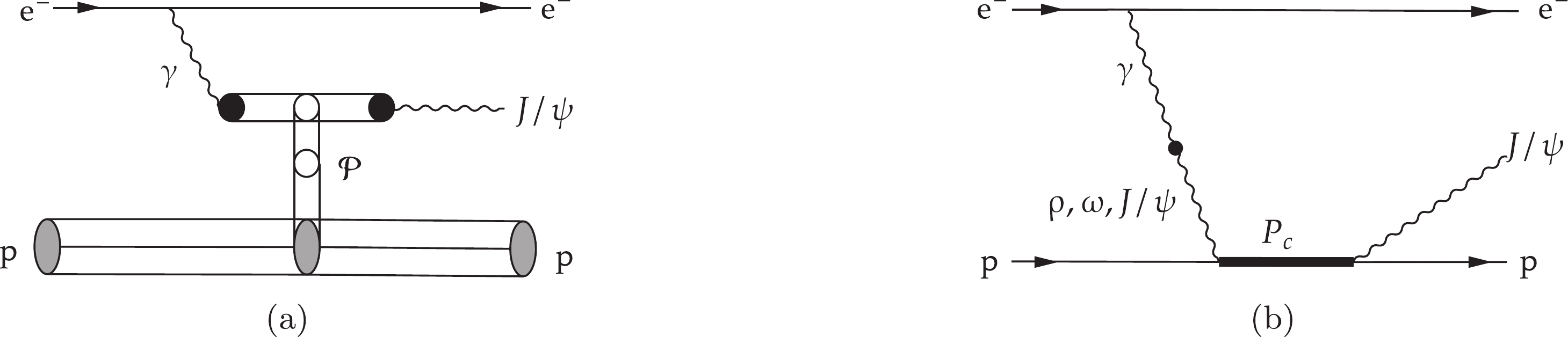

Figure 2.  Mechanisms of the interaction $e+p\rightarrow e +J/\psi+p$ for (a) background channel and (b) signal channel.

The amplitude ${\cal{M}}$ of the process $e+p\to e+J/\psi +p$ can be written as

where ${\cal{M}}^\mu_{R_1}$ and ${\cal{M}}^\nu_{R_2}$ denote the amplitudes of subprocess $e\rightarrow e\gamma$ and $\gamma p\rightarrow pJ/\psi$, respectively. ${\cal{M}}^\mu_{R_1}$ can be obtained straightforwardly from quantum electrodynamic theory:

where $u_e$ is the spinor of the electron, $k(k^\prime)$is the four-momentum and $\lambda$ is the z-component of the spin, with unprimed variables for the incoming electron and primed variables for the outgoing electron. ${\cal{M}}^\nu_{R_2}$ includes two parts corresponding to the different mechanisms:

where $p, p', q, q'$ are the four-momenta of the initial proton, final proton, intermediate proton, and $J/\psi$, respectively; and $m_s, m'_s, \lambda'_{J/\psi}$ are the z-component of spin of the initial proton, final proton and$J/\psi$, respectively. In addition, $u_p$ and $\epsilon^\mu$ denote the spinor and polarization vector of the proton and $J/\psi$, respectively. The two terms ${\cal{M}}^{\mu \nu}_{\mathbb{P}}$ and ${\cal{M}}^{\mu \nu}_{P_c}$ are the amplitudes for the $\gamma + p \to J/\psi + p$ by Pomeron exchange and the $P_c$ resonances, respectively.

The Pomeron exchange diagram is regarded as the background channel. The detailed derivation of ${\cal{M}}^{\mu\nu}_\mathbb{P}$ can be found in Ref. [11]. Here we just list the resulting definitions:

where $G_{\mathbb{P}}$ is the propagator of the Pomeron with $\alpha^\prime_p= 1/S_0=0.25$ GeV^-2 and $\alpha_0=1.25$. $\beta_{u/d/c}$ is the coupling between the Pomeron and the quark in the hadron, with $\beta_{u/d}=2.07$ GeV^-1 and $\beta_{c}=0.84$ GeV^-1. The form factors $F_{J/\psi}$ and $F_N$ are for the interaction of Pomeron with $J/\psi$ and N respectively, where $\mu_0=1.1$ GeV and $t=(p-p^\prime)^2$ is in unit of GeV².

For the signal channel, the amplitude ${\cal{M}}^{\mu \nu}_{P_c}$ is given by the assumption that the spin of $P_c$ is 1/2 with negative parity.

where $\tilde{g}^{\mu\nu} = g^{\mu\nu} - \dfrac{(p+q)^\nu (p+q)^\nu}{(p+q)^2}$, $r^\mu =p ^\mu-q^\mu$, $\tilde{\gamma}^\nu = \gamma_{\mu}\tilde{g}^{\mu\nu}$, $\tilde{r}^\nu = r_\mu\tilde{g}^{\mu\nu}$. $F_V(q^2)$ is the off-shell form factor for the intermediate vector,

where cut-off $\Lambda_V$ is an undetermined parameter as discussed in Ref. [11]. For simplification, this factor will be dealt with as a constant, since the main contribution will be around $q^2\sim 0$ GeV² because of the photon propagator. Here the aim is to find out the kinematic range for largest signal of $P_c$ states, thus we neglect the interference between the above two mechanisms and the overall constant factors are just taken as 1 for simplification.

The amplitudes can be calculated from the equations above, then the proper set of IKVs is chosen for the best phase space range of the signal of $P_c$ states. For a three-body final state, there are three sets of IKVs for $e+p\rightarrow e+J/\psi+p$ as shown in Tables 1–3. To make the regions minimally overlap between the two mechanisms, variables ${\rm{d}} m^2_{pJ\psi}$,${\rm{d}} m^2_{eJ/\psi}$, ${\rm{d}}\alpha$,${\rm{d}}(\cos\beta)$, and ${\rm{d}}\gamma$ are the most appropriate choices and the z-axis of coordinate frame is along the direction of initial proton. Typically, the indexes of the final state proton, electron, and $J/\psi$ are set as particle 1, 2, and 3, respectively, then the physical meaning of the Euler angles can be clear and the IKVs are set the same as those in Table 1. It is worth mentioning that β can be recognized as the angle between the initial and final protons. Furthermore, because of the axial symmetry for the scattering process, ${\rm{d}}\alpha$ can be trivially integrated out and one can obtain the factor $2\pi$. On the other hand, ${\rm{d}}\gamma$ will be integrated through the Gaussian quadrature method for the case here, because it's hard to measure directly. The remaining kinematic variables are $m^2_{pJ/\psi}$, $m^2_{eJ/\psi}$, $\cos\beta$ and the phase space is now three-dimensional. The distribution of $|{\cal{M}}_{ep\rightarrow eVp}|^2{\rm{d}}\Phi_{4}/{\rm{d}} m^2_{pJ/\psi}{\rm{d}} m^2_{eJ/\psi}{\rm{d}} \cos\beta$ is straightforwardly computed as a three-dimensional plot with variables $m^2_{pJ/\psi}$, $m^2_{eJ/\psi}$, and $\cos\beta$.

In order to show significant phase space range for two mechanisms, three-dimensional distribution plots are shown in Fig. 3 with the center-of-mass energy being 18 GeV, which will be available at EicC in the future. Red and green scatters stand for signal channel and background channel, respectively. The density of scatter in the neighborhood of a point in the phase space indicates the order of magnitude of the differential cross section at that point. Actually, since there is a huge magnitude difference in the differential cross sections for different ranges, we only draw the main contribution component and leave the other blank. Clearly, $P_c$ signals are mainly enhanced on the boundary between two invariant mass variables. It is easy to understand that the signal events will concentrate around the mass of the $P_c$ state because of its narrow width. On the other hand, the background signals concentrate in the range of $\beta \sim 0$ and decrease quickly for larger β. This results from the exponential term in ${\cal{M}}_{\mathbb{P}}^{\mu\nu}$. Then by this diagram, we find that the best kinematic interval for extracting the pentaquark signal for the process $e+p\rightarrow e+J/\psi+p$ requires the following conditions. The energy of the outgoing electron should be larger than 8 GeV, as calculated from the limitation of invariant mass of the $J/\psi p$ system. The scattering angle of the proton should be between 11° and 55° to avoid background interference. The directions of the outgoing proton and outgoing electron are almost anti-parallel because the main contributions are from the edge of the Dalitz plot of $m^2_{pJ/\psi}$ and $m^2_{eJ/\psi}$.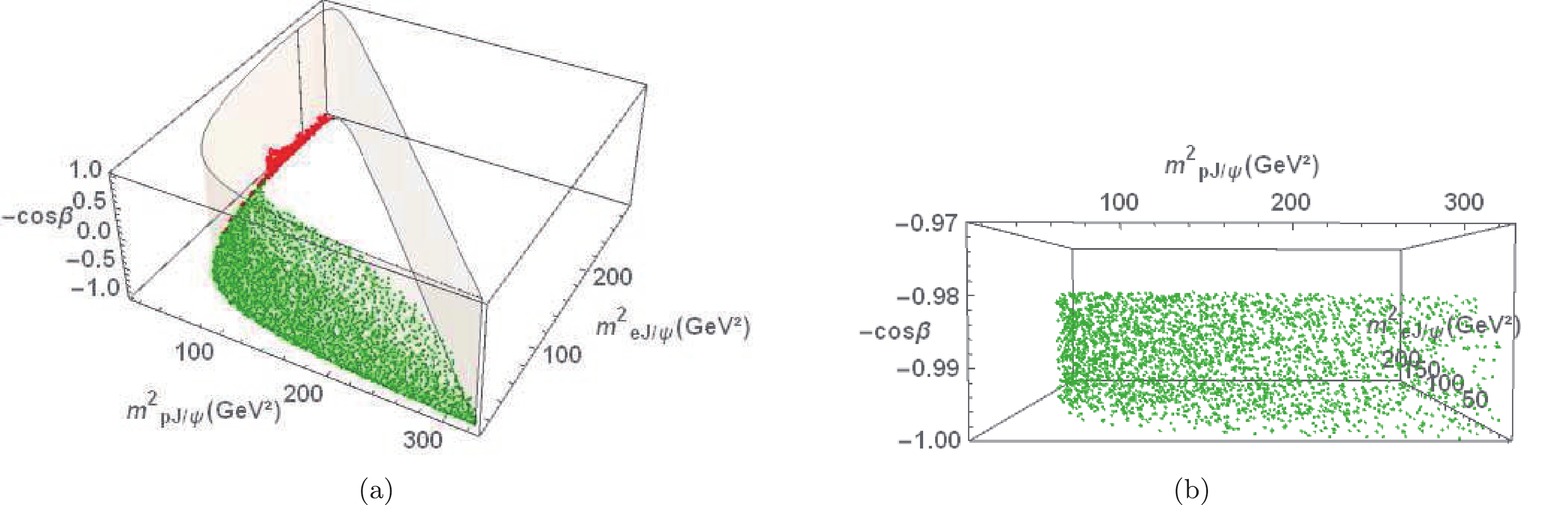

Figure 3.  (color online) Distributions of two channels with the center-of-mass energy being 18 GeV. The density of scatter in the neighborhood of a point in the phase space indicates the order of magnitude of the differential cross section at that point. Regions with no scatter mean that cross sections in that region are at least $10^4$ times smaller than the maximum. (a) Distribution of two channels where red scatter stands for the signal channel while green scatter stands for the background channel. (b) Distribution of background channel in a detailed scale of $-\cos\beta$.

In the previous three-body case, we found that the resonant peak will be buried in the huge background. It is necessary to find a typical kinematic region to isolate the resonance. For the four-body case, there are many more possible choices of IKVs than in the three-body case. Thus, it is important to choose a proper set of variables for extracting the information of a typical resonance.

As mentioned before, the invariant mass spectrum is usually useful for extracting the mass and width of the resonance, however, in some cases the resonance peak is not directly seen in the invariant mass spectrum for a reaction with several different mechanisms. To illustrate, we provide a toy model for $J/\psi \to \eta\pi^+\pi^-\phi$ reaction here. Since the aim is just to show the importance of choosing proper kinematic variables, we simply assume that the Feynman diagrams for the reaction are just the three tree diagrams shown in Fig. 4. For each diagram, there are two resonances. To avoid overcomplicated amplitudes, we use Breit–Winger propagators of each resonance for the amplitude of each diagram,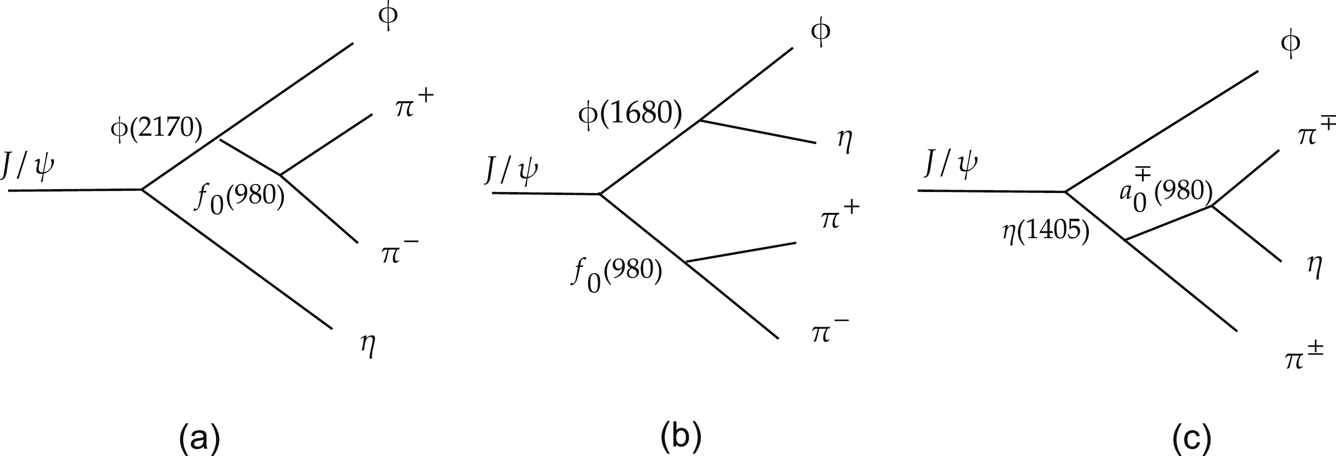

Figure 4.  Three tree diagrams of reaction $J/\psi \to \eta\pi^+\pi^-\phi$.

where $p_R$, $m_R$, and $\Gamma_R$ are the four-momentum, mass, and width of the resonance R. The mass and width parameters are listed in Table 27, which are roughly consistent with the values in the RPP. The additional factor ${1}/{2}$ is used to weaken the contribution of the first diagram.

R	$\phi(2170)$	$\phi(1680)$	$f_0(980)$	$a^\pm_0(980)$	$\eta(1405)$
mass	2157	1680	980	980	1405
width	100	100	70	70	100

Table 27.  Parameters used in Eq. (53), with unit MeV.

Furthermore, we recognize Fig. 4(a) as the signal channel and the other two mechanisms are both background. The task is to find a proper way to show the explicit peak of $\phi(2170)$. Since in this amplitude the variables are all invariant masses, the IKVs shown in Table 5 are the most convenient choices. Here, $\pi^+$, $\pi^-$, η, and ϕ are recognized as particle 1, 2, 3, and 4, respectively. Various Dalitz plots are shown in Fig. 5. From these Daliz plots, it is clear that the background channels will interfere with the peak structure of $\phi(2170)$. Indeed, from Fig. 6, it is found that the typical peak of $\phi(2170)$ resonance is buried in the distribution ${\rm{d}} N/{\rm{d}} m^2_{\phi\pi\pi}$, shown in Fig. 6 by the black solid line. On the other hand, from Fig. 5(b) and (c) one can easily find that a cut of $m^2_{\eta\pi^\pm}$ is necessary for a clean peak of $\phi(2170)$. Therefore, with a cut $m^2_{\eta\pi^\pm}>1.25$ GeV², a clear peak can be found, as shown in Fig. 6 by the dashed line. This is a very simple example to show the importance of finding a proper kinematic region to extract information about the resonance. In a more realistic case, things are much more complicated since the amplitudes can be dependent on various angles by including the high partial wave contributions. At that time, we believe that this set of IKVs including five invariant masses may not the best choice to search the proper kinematic region; other IKV sets should be useful.

Figure 5.  Daliz plots of invariant mass squared of $\phi\pi^+\pi^-$ vs invariant mass squared of $\pi^+\pi^-$, $\eta\pi^+$, $\eta\pi^-$ and $\phi\pi^+$ for reaction $J/\psi \to \eta\pi^+\pi^-\phi$.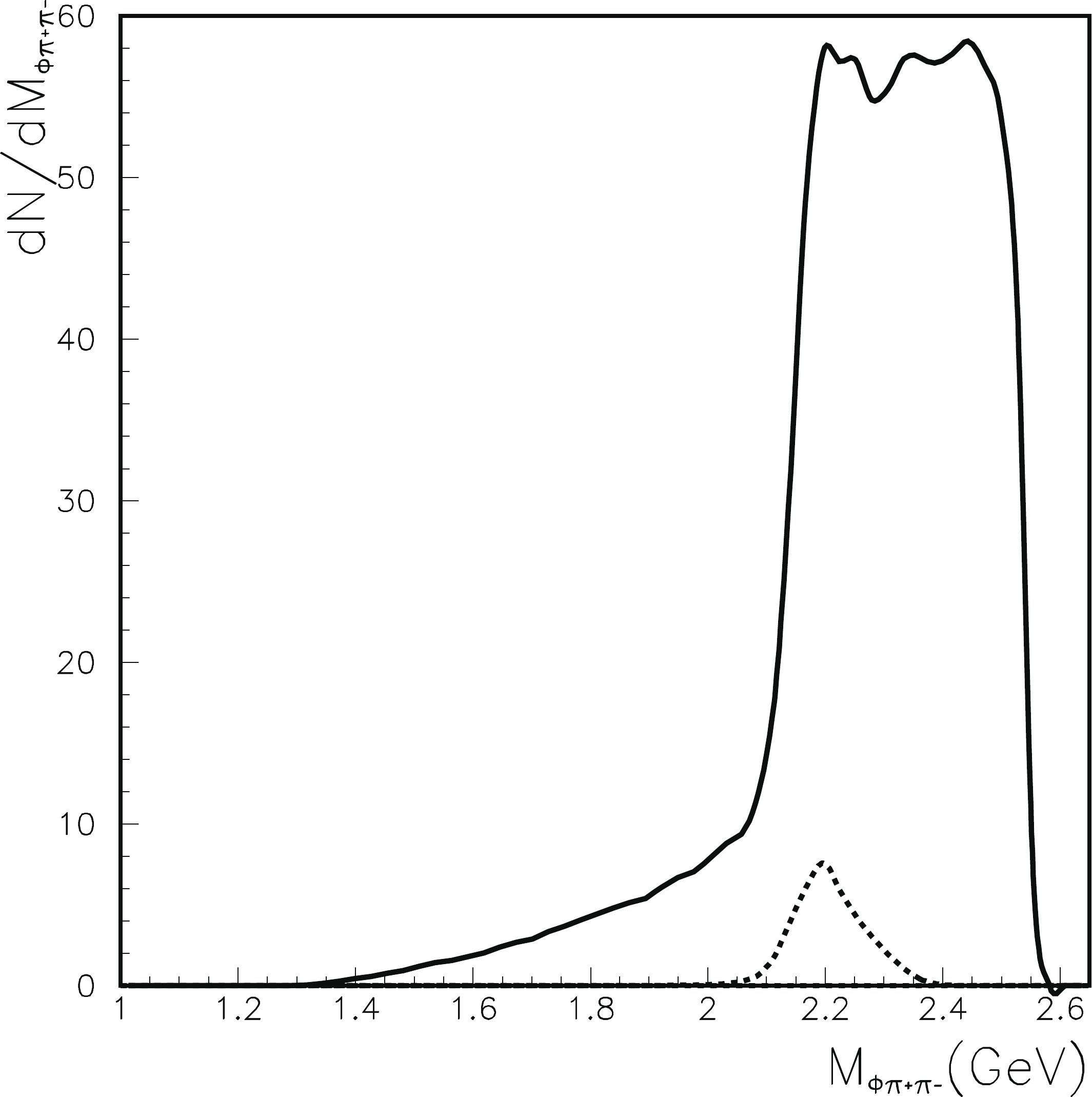

Figure 6.  Invariant mass spectrum of $\phi\pi^+\pi^-$ for reaction $J/\psi \to \eta\pi^+\pi^-\phi$. ${\rm d} N/{\rm d} m_\phi\pi^+\pi^-$ is normalized to the 1000 events of this process. The solid line is the distribution with all contributions and the dashed line has a cut $m^2_{\eta\pi^\pm}>1.25$ GeV².

In this paper, all unique sets of kinematic variables containing a certain number of invariant masses are enumerated and classified for three- and four-body final states. Expressions of phase space factor as well as four-momenta for each case are explicitly shown. The formulae given in this paper are especially useful for extracting the structure of resonances. As an example of application, we calculate the process $e+p\to e+J/\psi+p$ and find out the region of phase space where the signal and background each reach their maxima, which will help experimental physicists to search for $P_c$ signal economically and effectively. Therefore, the formulae in this paper should be useful for the further research on three- and four-body final state processes. Moreover, the method provided in this paper can also be used for any n-body final state processes. Furthermore, the method developed here can be used in the case that the intermediate particle is on shell. Typically, if this happens in the tree diagram, such intermediate particles can be cut for the final state of the former process and the initial state of the continue process. Then the whole process can be divided into two processes, where three- and four-body phase spaces are also applied for each, as discussed in Ref. [13]. If this happens in the loop integral, the loop momentum can be recognized as a phase space integration momentum. So our phase space integration method can also be used in the on-shell loop integration. This may combine with some useful techniques such as sector-decomposition [13].

The authors would like to thank Hao-Jie Jing, Feng-Kun Guo, Yan-Ping Huang, and Bing-Song Zou for helpful discussions.