The cross-section for the ${{\boldsymbol\gamma e}^{\bf -} {\bf\rightarrow} {\boldsymbol Ze}^{\bf -} {\bf\rightarrow}{\boldsymbol l}^{\bf -} {\boldsymbol l}^{\bf +}{\boldsymbol e}^{\bf -} }$ scattering at the LHeC

Electro-weak and strong interactions have been unified in the Standard model (SM). The discovery of the Higgs signal at the Large Hadron Collider (LHC) completed the particle spectrum of the SM. However, the existence of some theoretical drawbacks in the SM has motivated the development of extended models. One of the most attractive extended models is the Randall-Sundrum (RS) model, which provides a new scenario with an extra dimension to naturally solve the gauge hierarchy [1]. Owing to the extra dimension, the additional scalar field called radion can be mixed with the Higgs boson [2–5]. The low mass radion region, even at 10 GeV, is worth investigating [6]. Besides SM couplings, anomalous couplings of the mixed radion and Higgs boson to $\gamma \gamma,~ ZZ,~ gg,~ \gamma Z$ have been considered.

It is important to test the electro-weak sector of the SM by studying Z boson production. Z production using the Compton backscattered photon was considered at the International Linear Collider (ILC) [7]. Recently, Z-pair production in hadron colliders has been investigated at the LHC [8–14]. However, the Large Hadron-electron Collider (LHeC), planned at the Large Hadron Collider (LHC), is a cleaner configuration [15–19]. Moreover, the center of mass energy at the LHeC is higher than that at the ILC. The incoming proton beam energy at the LHeC is set to $E_{p} = 7$ TeV and the center of mass energy is given by$\sqrt{s} = 2\sqrt{E_{p}E_{e}}$. The LHeC plans to collide electrons with energy ranging from 60 GeV to 140 GeV [20]. Therefore, it can provide better conditions for researching new phenomena compared to the LHC and ILC. The LHeC may play a significant role in the pursuit of new physics beyond the SM [21]. $\gamma e^{-}$ collisions with the photon beam radiated from the proton provides an extra experimental scenario to help reduce the background [22]. In spite of a lower luminosity, the $\gamma e^{-}$ subprocess can be studied as a complementary tool to $e^{-} p$ collision at the LHeC.

In the present study, we analyzed the subprocess $\gamma e^{-} \rightarrow Ze^{-} \rightarrow l^{-} l^{+} e^{-}$, including the vertices of Z boson such as $\gamma ZZ$, $\gamma\gamma Z$, $\gamma Zh$, and $\gamma Z \phi$. With the contribution of new interactions in the RS model, including radion and Higgs propagators, the total cross-section was expected to be experimentally detected. The organization of this paper is as follows. In Section II, we review the Randall-Sundrum model and the mixing of Higgs - radion. The cross-section for $\gamma e^{-} \rightarrow Ze^{-} \rightarrow l^{-} l^{+} e^{-}$ collisions at the LHeC is presented in Section III. Finally, we summarize our results and draw conclusions in Section IV.

The RS model consists of one extra dimension bounded by two 3-branes. The UV-brane, whose fifth dimension is bounded, is located at $y = 0$, whereas the IR-brane is located at $y = \pi r_{c}$. The five dimensional metric has the following form:

where $b_{0}$ is a length parameter for the fifth dimension, $r_{c}$ is the compactification radius, and k is the curvature of the five dimensional geometry. The exponential function represents the warp factor that generates the gauge hierarchy. The values of the bare parameters are determined by the Planck scale and the applicable value for the size of the extra dimension is assessed by $kr_{c} \simeq 11 - 12$. Thus, the weak and gravity scales can be naturally generated. The relation $\overline{M}_{Pl}^{2} = M_{5}^{3}/k$ is derived from the 5D action. The scale of physical phenomena on the IR-brane is given by $\Lambda_{\phi} \equiv \overline{M}_{Pl} {\rm e}^{-kr_{c}\pi}$ with $\Lambda _{\phi } \sim$ few TeV. The mass of the $n^{\rm th}$ KK graviton excitation is $m^{G}_{n} = x_{n}^{G}k\Lambda_{\phi}/\overline{M}_{Pl}$, with $x_{n}^{G}$ being the roots of the $J_{1}$ Bessel function [23]. The coupling strength of the graviton KK states to the SM fields is $\Lambda_{\phi}^{-1}$. The gravity-matter interactions are expressed as [24]

where $h^{n}_{\mu\nu} (x)$ denotes the Kaluza-Klein (KK) modes of the graviton field $h_{\mu \nu}(x, y)$, $\phi_{0} (x)$ is the radion field, $\Lambda_{\phi} \equiv \sqrt{6}M_{Pl}\Omega_{0}$ is the VEV of the radion field, and $\hat{\Lambda}_{W} \equiv \sqrt{2}M_{Pl}\Omega_{0}$.$T^{\mu\nu}$ is the energy-momentum tensor, which is given at the tree level [25, 26] as follows:

The gravity-scalar mixing is described by the following action [27]:

where ξ is the mixing parameter, $R(g_{\rm vis})$ is the Ricci scalar for the metric $g_{vis}^{\mu \nu } =\Omega _{b}^{2} (x)(\eta ^{\mu \nu } +\varepsilon h^{\mu \nu } )$ induced on the visible brane, $\Omega _{b} (x) = {\rm e}^{-kr_{c} \pi} (1 + \frac{\phi_{0}}{\Lambda _{\phi }})$ is the warp factor, and $\hat{H}$ is the Higgs field in the 5D context before rescaling to canonical normalization on the brane. With $\xi \ne 0$, there is neither a pure Higgs boson nor a pure radion mass eigenstate. This ξ term mixes $h_{0}$ and $\phi_{0}$ into the mass eigenstates h and ϕ as follows:

where $Z^{2} = 1 + 6\gamma ^{2} \xi \left(1 -\, \, 6\xi \right) = \beta - 36\xi ^{2}\gamma ^{2}$ is the coefficient of the radion kinetic term after undoing the kinetic mixing, $\gamma = \upsilon /\Lambda _{\phi },~ \upsilon = 246$ GeV, $a = -\dfrac{\cos\theta}{Z},~ b = \dfrac{\sin\theta}{Z},~ c = \sin\theta + \dfrac{6\xi\gamma}{Z}\cos\theta, ~ d = \cos\theta - \dfrac{6\xi\gamma}{Z}\sin\theta$. The mixing angle θ is expressed as

where $m_{h_{0}}$ and $m_{\phi _{0}}$ are the Higgs and radion masses before mixing, respectively.

The new physical fields h and ϕ in (5) are the Higgs-dominated state and radion, respectively:

There are four independent parameters, namely $\Lambda _{\phi } ,\, \, m_{h} ,\, \, m_{\phi } ,\, \, \xi$, that must be specified to fix the state mixing parameters. We consider the case of $\Lambda _{\phi } = 5$ TeV and $\dfrac{m_{0} }{M_{P} } = 0.1$, which makes the radion stabilization model most natural [26].

Feynman rules for couplings in the RS model are expressed as follows [6]:

where a, b, c, d are the state mixing parameters in the RS model; $g_{h} = d + \gamma b$, $g_{\phi} = c + \gamma a$, $g_{h}^{r} = \gamma b$, $g_{\phi}^{r} = \gamma a$; the triangle loop functions $A_{F}, A_{W}$ are given in Ref. [28]

We consider a collision process in which the initial state contains an electron and a photon emitted from proton beams, and the final state contains a Z boson and an electron:

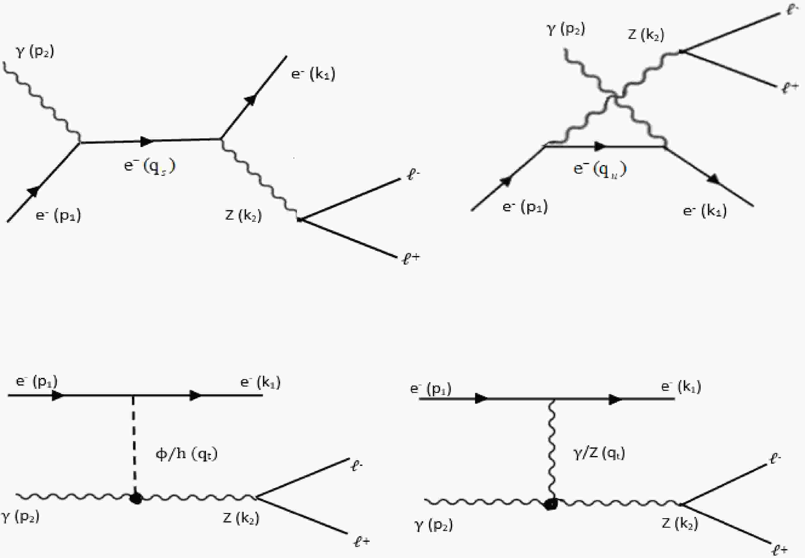
Here, $p_{i}, k_{i}$ (i = 1, 2) represent the momentums. Three Feynman diagrams contribute to the reaction expressed in (12), representing the s, u, t-channel exchange, as depicted in Fig. 1.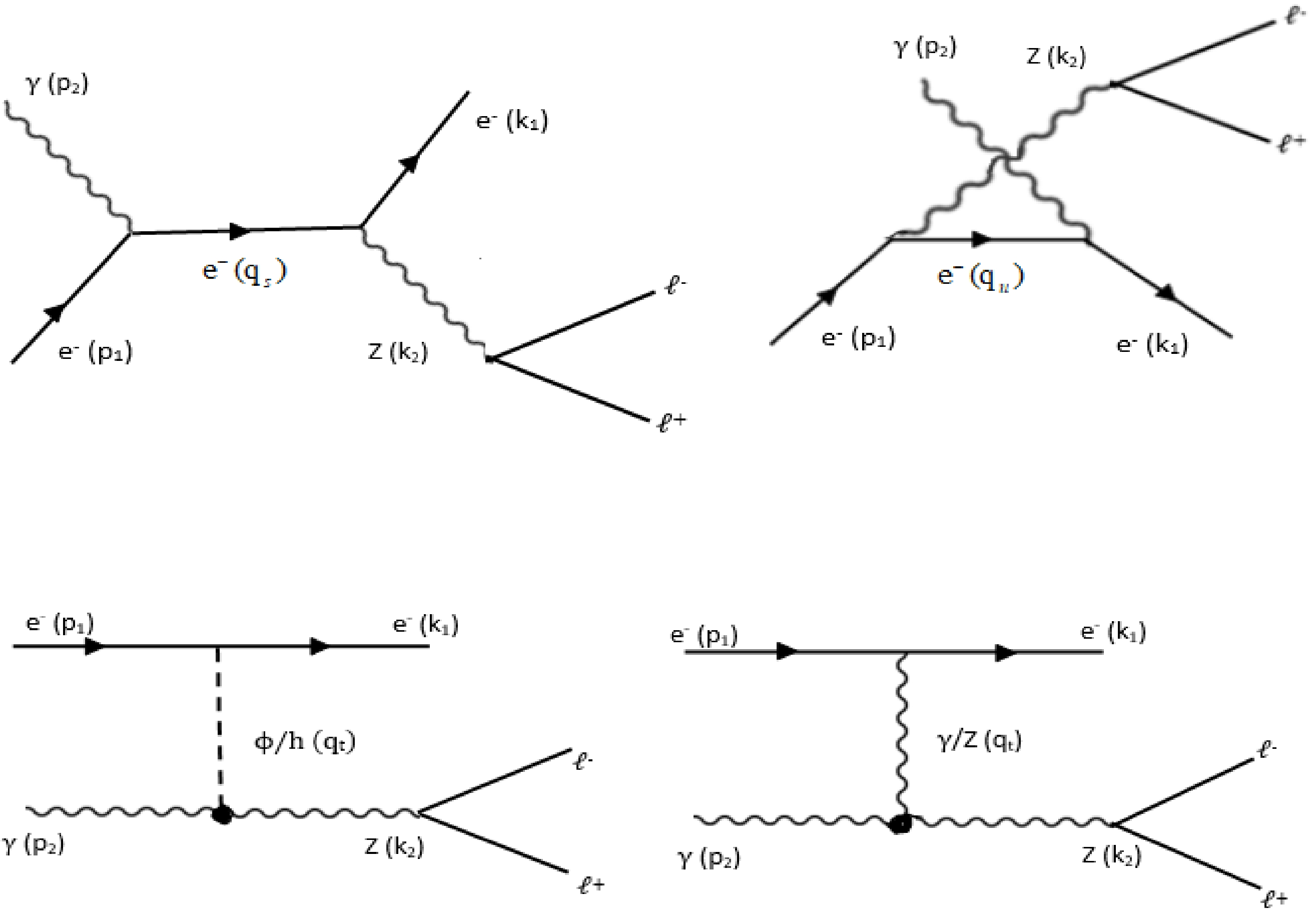

Figure 1.  Feynman diagrams for $\gamma e^{-} \rightarrow Ze^{-} \rightarrow l^{-} l^{+} e^{-}$ collisions, representing the s, u, t-channels, respectively.

The transition amplitude representing the s-channel is given by

The transition amplitude representing the u-channel can be written as

The transition amplitude representing the t-channel is given by

where

The triple gauge boson couplings are given by [14]

The total cross-section for the whole process can be calculated as follows:

The effective production cross-section for the subprocess at the LHeC can be described as follows [22]:

where

is the expressions of the differential cross-section [29], $\widehat{s} = 4E_{e}E_{\gamma} = \xi s$ is center of mass energy of the sub-process $\gamma e^{-} \rightarrow Z e^{-}$, and $\psi = (\widehat{\overrightarrow{p}_{1}, \overrightarrow{k}_{2}})$ is the scattering angle. The photon flux can be written as

where

with

$M_{P}$ is the mass of the proton; $E_{p}$ is the energy of the incoming proton beam; $E_{\gamma} = \xi E_{p}$ is the photon energy, which is related to the loss energy of the emitted proton beam;$F_{E}, F_{M}$ are functions of the electric and magnetic form factors given in the dipole approximation; and $\mu^{2}_{P} = 7.78$ is the magnetic moment of the proton.

For numerical evaluation, we set the energy of the incoming proton beam at the LHeC, that is, $E_{p} = 7$ TeV, and an electron beam energy $E_{e}$ in the range of 60 GeV $\leq E_{e} \leq 140$ GeV [20]. The vacuum expectation value (VEV) of the radion field was set as $\Lambda_{\phi} = 5$ (TeV) [27]. The radion mass was set as $m_{\phi} = 10$ GeV [30]. The Higgs mass was set as $m_{h} = 125$ GeV (CMS). The maximum value of anomalous couplings in the tightest limits with the corresponding observable were set as $f_{4}^{\gamma} = 2.4 \times 10^{-3}$, $f_{5}^{\gamma} = 2.7 \times 10^{-3}$, $h_{1}^{\gamma} = 3.6 \times 10^{-3}$, $h_{3}^{\gamma} = 1.3 \times 10^{-3}$ [14]. The polarization coefficients of the initial and final $e^{-}$ beams were set as $P_{1} = P_{2} = 0.8$, respectively [17]. Given that the contribution to the above integral formula is very small for $Q^{2}_{\max} > 2~\rm GeV^{2}$, $Q^{2}_{\max}$ was set as 2 $\rm GeV^{2}$ [22]. We next provide estimates for the cross-sections:

i) The electron beam energy was set as $E_{e} = 60$ GeV. In Fig. 2, we plot the differential cross-section as a function of$\cos\psi$. This figure shows that ${\rm d}\sigma/{\rm d}\cos\psi$ peaks in the forward direction and becomes flat in the backward direction.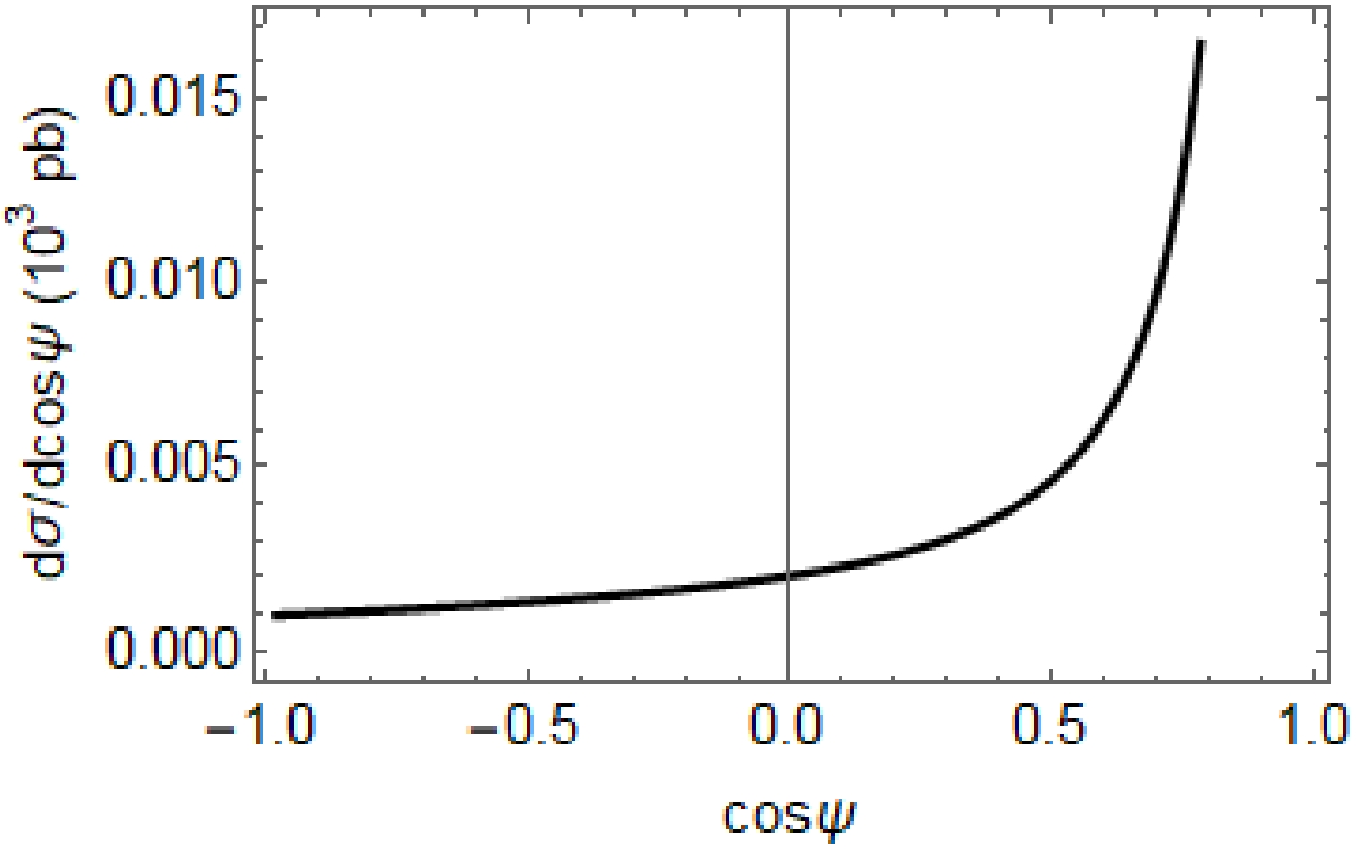

Figure 2.  Differential cross-section as a function of$\cos\psi$. The parameters were set as $P_{1} = P_{2} = 0.8$, $E_{e}$ = 60 GeV.

ii) In Fig. 3, the forward-backward asymmetry is plotted as a function of $E_{e}$. This figure indicates that the forward-backward asymmetry decreases when the electron beam energy increases.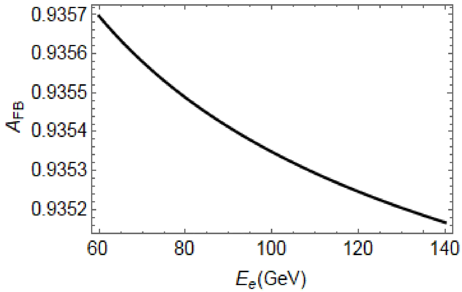

Figure 3.  Forward-backward asymmetry as a function of the electron beam energy $E_{e}$. The parameters were set as $P_{1} = P_{2} = 0.8$.

iii) In Fig. 4, we evaluate the dependence of the total cross-section on the initial and final electron beam in the case of $E_{e} = 60$ GeV. The cross-section achieves its maximum value when both the initial and final electron beams are left or right polarized $(P_{1} = P_{2} = \pm 1)$. The cross-section reaches its minimum value when $P_{1} = 1$, $P_{2} = -1$ and vice versa. It is worth noting that the cross-section in the case of both left and right polarized initial and final electron beams is twice as much as the unpolarized electron beams.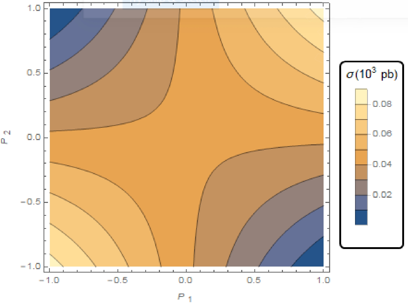

Figure 4.  (color online) Total cross-section as a function of the polarization coefficients of the initial and final electron beam. The electron beam energy was set as $E_{e} = 60$ GeV.

iv) In Fig. 5, we evaluate the dependence of the total cross-section on the electron beam energy $E_{e}$. The electron beam energy was set in the range of 60 GeV$\leq E_{e} \leq$ 140 GeV. Here, the polarization coefficients of the initial and final electron beams were set as $P_{1} = P_{2} =$ 0.8, 0.6, 0. The figure shows that the total cross-sections increase when the electron beam energy $E_{e}$ increases. In Table 1, some typical values for the total cross-section are listed. We emphasize that the main contribution to the description process is from the s, u-channels, while the anomalous couplings for the contribution are very small. However, the anomalous couplings concerning mixing of Higgs-radion need to be further studied.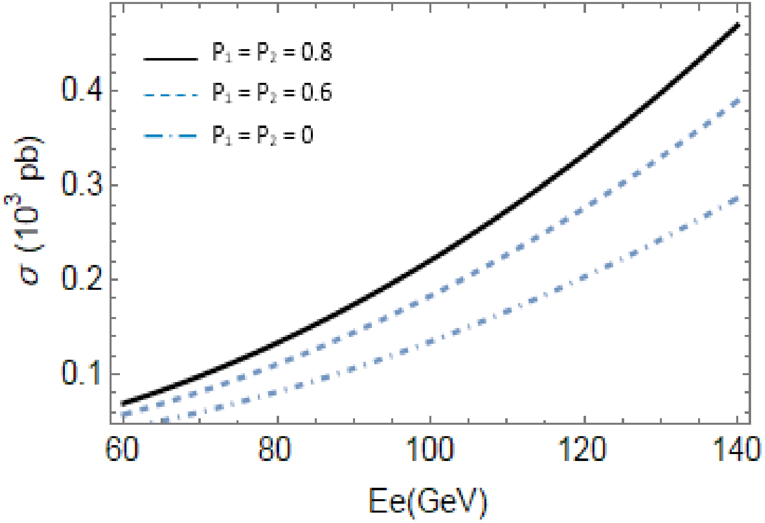

Figure 5.  Total cross-sections as a function of the electron beam energy $E_{e}$ for polarization coefficients $P_{1} = P_{2} =$ 0.8, 0.6, 0.

$E_{e}$/GeV	60	70	80	90	100	110	120	130	140
σ($P_{1} = P_{2} = 0.8$) ($10^{3}\rm pb$)	0.069	0.098	0.133	0.174	0.221	0.274	0.333	0.399	0.471
σ($P_{1} = P_{2} = 0.6$) ($10^{3}\rm pb$)	0.057	0.081	0.110	0.144	0.183	0.227	0.276	0.331	0.390
σ($P_{1} = P_{2} = 0$) ($10^{3}\rm pb$)	0.042	0.059	0.081	0.106	0.135	0.167	0.203	0.243	0.287

Table 1.  Typical values for the total cross-section in $\gamma e^{-} \rightarrow Z e^{-} \rightarrow l^{-}l^{+}e^{-}$ collisions at the LHeC.

In this study, we evaluated the total cross-section in $\gamma e^{-} \rightarrow Z e^{-} \rightarrow l^{-}l^{+}e^{-}$ production at the LHeC using the RS model. The results show that the main contribution to the description process is from the s, u-channels, while the anomalous couplings for the contribution are very small. Note that the Z boson with such a short lifetime is never seen directly in the experiments. Although the branching ratio of $Z \rightarrow l^{-}l^{+}$ is fairly small, the $l^{-}l^{+}$ channel leaves a relatively clean signature in the detector, which allows the process to be measured with higher accuracy [31]. In this study, our focus was on the comparison between the cross-sections at the ILC and LHeC. The value at the ILC was described in detail in Ref. [7]. It is concluded that the total cross-section in $\gamma e^{-} \rightarrow Z e^{-} \rightarrow l^{-}l^{+}e^{-}$ at the LHeC is much larger than that at the ILC.

Finally, we emphasize that the scalar anomalous couplings concerning mixing of Higgs- radion in the RS model need to be further investigated.