


 Abstract
 HTML
HTML Reference
 Related
 PDF
PDF


-
The CDF-II Collaboration recently reported their new measurement of the W-boson mass [1]:
$ \begin{equation} M_{W,{\rm CDF\rm-II}}=80.4335 \pm 0.0094\enspace {\rm GeV}\,. \end{equation} $

(1) However, the most recent prediction of
$ M_W $ in the standard model (SM) is [2]$ \begin{equation} M_{W,{\rm SM}}=80.357 \pm 0.006\enspace {\rm GeV}\,. \end{equation} $

(2) Thus, it is clear that the discrepancy between the latest CDF-II value and SM calculation of
$ M_W $ exceeds the 7σ confidence level (CL.). If this$ M_W $ anomaly is further confirmed in the future, it would provide us with a novel hint of new physics (NP) beyond the SM (BSM). In literature, there have been many BSM attempts [3–129] to explain the$ M_W $ discrepancy. Among various BSM scenarios, the extension of the SM Higgs sector by introducing an additional$ SU(2)_L $ multiplet [3–43] is a promising direction. On the one hand, modification of the scalar sector is intimately related to the true mechanism of electroweak (EW) gauge symmetry breaking and the associated hierarchy problem, which might be probed by measuring the EW oblique parameters [130–135] and trilinear Higgs coupling [136–140]. On the other hand, the introduced scalar multiplet may solve many puzzles in the SM, such as the nature of dark matter (DM) [141–146], the generation of matter-anti-matter asymmetry in the Universe [147–150], and the characteristics of the EW phase transition and its associated stochastic gravitational wave signals [151–168]. Therefore, unveiling the structure of the scalar sector may help deepen our understanding of the overall picture of the SM and the physics beyond it.In light of the potential importance of the scalar multiplet extension of the SM, we focus on its solution for the W-boson mass anomaly. Note that previous studies have only concentrated on several specific models by including a scalar singlet [3–6], the second Higgs doublet [7–25], and a scalar triplet with
$ Y=0 $ or$ 1 $ [26–42]. In this study, instead of studying a particular model, we vary the EW$S U(2)_L$ isospin representation J and the hypercharge Y of the additional scalar in the absence of its vacuum expectation value (VEV) and observe their effects on the interpretation of the CDF-II W-boson excess. When the scalar multiplet does not carry any VEV1 , the dominant contributions to the W-mass correction are provided by those at the one-loop level, which can be represented as the linear combination of the EW oblique parameters T and S [92, 94]. Thus, we first rederive the analytic formulae for T and S from a general scalar multiplet, confirming the results on$ M_W $ in literature. We then apply these simple expressions to several scenarios of physical interest, such as a real or complex multiplet with$ Y=0 $ , cases with$ J=Y $ , and the variation of Y with a fixed J. In our phenomenological studies, we also consider the constraints from EW global fits and perturbativity, which directly constrain the present scalar models.The paper is organized as follows: In Sec. II, we begin by setting the notation of a general
$S U(2)_{L}$ scalar multiplet and its relevant terms in the Lagrangian interacting with SM gauge and Higgs doublet bosons. We also give the general formulae for its one-loop contribution to the W-boson mass, which can be expressed as linear combinations of the oblique parameters T and S at leading order. In Sec. III, we study several specific models of great physical interest in the scalar-multiplet extensions of the SM and explore their ability to explain the observed$ M_W $ anomaly by varying the scalar$S U(2)_L$ representations and hypercharges, where we also consider the constraints from the perturbativity and EW global fits. We conclude in Sec. IV, where we briefly discuss the possible collider signatures of additional scalars, especially when the dimension of the scalar multiplet is high. In addition, we include several appendices. In Appendix A, we give the relevant part of the Lagrangian and associated Feynman rules involving the scalar multiplet. In Appendix B, we show that two particular terms in the scalar potential can be represented as linear combinations of other existing terms, resulting in them being ignored in the subsequent discussion. In Appendix C, we define several functions relating to the one-loop contributions of the scalar multiplet to the oblique parameters T and S. Finally, in Appendix D, we give the calculation details from when we rederive the one-loop expressions of the T and S parameters from a scalar multiplet with general EW charges. -
Generally, we label the scalar multiplet as
$ \Phi_{JY} $ , where J denotes the weak isospin$S U(2)_L$ representation, and Y is the hypercharge, so that the dimension of the multiplet is$ N=2J+1 $ . We also label the components in the scalar multiplet$ \Phi_{JY} $ as$ \Phi_{I}^{Q} $ :$ \Phi_{JY}=\left(\begin{array}{c} ...\\ \varPhi_{I}^{Q}\\ ... \end{array}\right), $

(3) where
$ I=J,J-1,J-2,......,-J+1,-J $ , and the electric charge$ Q=I+Y $ .The EW covariant derivative after EW symmetry breaking can be written as
$ D_{\mu}=\partial_{\mu}+{\rm i}eQA_{\mu}+{\rm i}\frac{g}{c_{W}}\left(T_{3}-Qs_{W}^{2}\right)Z_{\mu}+{\rm i}g\left(W_{\mu}^+T_++W_{\mu}^-T_-\right), $

(4) where
$ T_{k}\; (k=1,2,3) $ are the three generators of the$ SU(2)_L $ group, and the ladder operator$ T_{\pm} $ is given by$ T_{\pm}=(T_{1} \pm iT_{2})/\sqrt{2} $ . The eigenvalues of$ T_{3} $ can be labeled using I as in Eq. (3). The actions of$ T_{3} $ and$ T_{\pm} $ on$ \Phi_{JY} $ are given by$ \begin{equation} T_{3}\Phi_{JY}=T_{3}\left(\begin{array}{c} ...\\ \varPhi_{I}^{Q}\\ ... \end{array}\right)=\left(\begin{array}{c} ...\\ I\varPhi_{I}^{Q}\\ ... \end{array}\right), \end{equation} $

(5) $ \begin{equation} T_+\Phi_{JY}=T_+\left(\begin{array}{c} ...\\ \varPhi_{I}^{Q}\\ ... \end{array}\right)=\left(\begin{array}{c} ...\\ N_{I}\varPhi_{I-1}^{Q}\\ ... \end{array}\right), \end{equation} $

(6) $ \begin{equation} T_-\Phi_{JY}=T_-\left(\begin{array}{c} ...\\ \varPhi_{I}^{Q}\\ ... \end{array}\right)=\left(\begin{array}{c} ...\\ N_{I+1}\varPhi_{I+1}^{Q}\\ ... \end{array}\right), \end{equation} $

(7) where
$ N_{I}=\sqrt{{(J+I)(J-I+1)}/{2}} $ , and we only show the element with the quantum number of$ T_3 $ equal to I in the multiplet. Then,$ D^{\mu}\Phi_{JY} $ can be written as$ \begin{aligned}[b] D^{\mu}\Phi_{JY}= &\partial^{\mu}\varPhi_{I}^{Q}+{\rm i} eQA_{\mu}\varPhi_{I}^{Q}+{\rm i}\frac{g}{c_{W}}\left(I-Qs_{W}^{2}\right)Z_{\mu}\varPhi_{I}^{Q}\\ &+{\rm i}gW_{\mu}^+N_{I}\varPhi_{I-1}^{Q}+{\rm i}gW_{\mu}^-N_{I+1}\varPhi_{I+1}^{Q}\,. \end{aligned} $

(8) The gauge interaction terms stemming from the kinetic term
$ \left(D_{\mu}\Phi_{JY}\right)^{\dagger}D^{\mu}\Phi_{JY} $ are shown explicitly in Appendix A.In this type of model, the potential constructed by the Higgs doublet H and scalar multiplet
$ \Phi_{JY} $ is given by$ \begin{aligned}[b] V\left(H,\Phi_{JY}\right)=&-\mu_{H}^{2}H^{\dagger}H+\lambda_{H}\left(H^{\dagger}H\right)^{2}+\mu_{\Phi_{JY}}^{2}\Phi_{JY}^{\dagger}\Phi_{JY}\\ &+\lambda_{1}\left(\Phi_{JY}^{\dagger}\Phi_{JY}\right)^{2}+\lambda_{2}\left(\Phi_{JY}^{\dagger}T_{\Phi}^{a}\Phi_{JY}\right)^{2}\\ &+\lambda_{3}\left(\Phi_{JY}^{\dagger}\Phi_{JY}\right)\left(H^{\dagger}H\right)\\ &+\lambda_{4}\left(\Phi_{JY}^{\dagger}T_{\Phi_{JY}}^{a}\Phi_{JY}\right)\left(H^{\dagger}T_{H}^{a}H\right)\\ &+\lambda_{5}\left(\Phi_{JY}^{\dagger}T_{\Phi_{JY}}^{a}T_{\Phi_{JY}}^{b}\Phi_{JY}\right)^{2}\,. \end{aligned} $

(9) Here, we only list the most general interaction terms for any scalar multiplet
$ \Phi_{JY} $ . Note that the potential in Eq. (9) respects$ Z_2 $ symmetry. When the dimension of the scalar multiplet is sufficiently high, there are no other terms at the renormalizable level; hence, this$ Z_2 $ symmetry becomes an accidental one at low energies. If the electrically neutral component is the lightest in the multiplet, it may provide us with a viable DM candidate that cannot decay owing to protection by this$ Z_2 $ symmetry. Such a scenario is known as minimal DM [141]. However, for certain specific$S U(2)_L \times U(1)_Y$ representations with low dimensions, there can be additional$ Z_2 $ -symmetry breaking terms. For example, in the Type-II seesaw model [169–174], a weak-isospin triplet with$ Y=1 $ ,$ \Phi_{1,1} $ , can give rise to the$ Z_2 $ -odd interaction as$ H^\dagger \Phi_{1,1} \tilde{H}+{\rm h.c.} $ , where$\tilde{H} \equiv {\rm i}\sigma_2 H^*$ , with$ H^* $ denoting the complex conjugate of the Higgs doublet H. Nevertheless, such$ Z_2 $ -odd terms are not relevant to our study on the one-loop corrections to the W-boson mass; therefore, we ignore them in the following. In addition, we can also write two other operators for any scalar multiplet:$ \begin{equation} O_6 + O_7 \equiv \lambda_{6}\left(H^{\dagger}\Phi_{JY}\right)\left(\Phi_{JY}^{\dagger}H\right)+\lambda_{7}\left|\widetilde{H}\Phi_{JY}\right|^{2}\,. \end{equation} $

(10) However, as shown in Appendix B, they are not independent because they can be represented as linear combinations of terms proportional to
$ \lambda_{3} $ and$ \lambda_{4} $ . Thus, neither of them can induce NP effects, as discussed later on. -
NP effects in the EW sector are usually imprinted by three oblique parameters, T, S, and U [130, 131]. In particular, the one-loop correction to the W-boson mass can be expressed as follows [130, 132, 133]:
$ \begin{equation} M_{W}=M_{W,SM}\left(1-\frac{\alpha\left(M_{Z}^{2}\right)}{4\left(c_{W}^{2}-s_{W}^{2}\right)}\left(S-2c_{W}^{2}T\right)+\frac{\alpha\left(M_{Z}^{2}\right)}{8s_{W}^{2}}U\right)\,, \end{equation} $

(11) where
$\alpha\equiv {\rm e}^{2}/(4\pi)=g^{2}s_{W}^{2}/(4\pi)$ is the fine-structure constant,$ s_{W}\equiv \sin\theta_{W} $ , and$ c_{W}\equiv\cos\theta_{W} $ , with$ \theta_{W} $ denoting the Weinberg angle. Here, the oblique parameters T, S, and U at the one-loop level are defined as2 $ \begin{aligned}[b] S\equiv&\frac{4s_{W}^{2}c_{W}^{2}}{\alpha}\left[A_{ZZ}^{\prime}\left(0\right)-\frac{c_{W}^{2}-s_{W}^{2}}{c_{W}s_{W}}A_{Z\gamma}^{\prime}\left(0\right)-A_{\gamma\gamma}^{\prime}\left(0\right)\right]\,, \\ T\equiv&\frac{1}{\alpha m_{Z}^{2}}\left[\frac{A_{WW}\left(0\right)}{c_{W}^{2}}-A_{ZZ}\left(0\right)\right]\,, \\ U\equiv&\frac{4s_{W}^{2}}{\alpha}\left[A_{WW}^{\prime}\left(0\right)-\frac{c_{W}}{s_{W}}A_{Z\gamma}^{\prime}\left(0\right)-A_{\gamma\gamma}^{\prime}\left(0\right)\right]-S\,, \end{aligned} $

(12) where the functions
$ A^{(\prime)}_{VV^\prime} (q^2) $ can be defined in terms of the vacuum polarization tensors for the EW gauge bosons$ V^{(\prime)} $ as follows:$ \begin{equation} \Pi_{VV^{'}}^{\mu\nu}\left(q\right)=g^{\mu\nu}A_{VV^{'}}\left(q^{2}\right)+q^{\mu}q^{\nu}A^\prime_{VV^{'}}\left(q^{2}\right)\,, \end{equation} $

(13) where q is the four-momentum of the corresponding vector bosons. However, as shown in Ref. [92], T and S are induced by dimension-6 operators, whereas U is induced by a dimension-8 operator so that it is significantly suppressed. Therefore, the dominant one-loop contribution to the W-boson mass is expected to be given by T and S for an NP model extended by a scalar multiplet, whereas the effect from U can be ignored. We explicitly check that when the added scalar masses are all larger than 300 GeV and their multiplet dimension is confined to be smaller than 10, the contribution of U to the W mass is always smaller than the leading ones from T and/or S by at least one order of magnitude, which confirms the above expectation. We return to this issue in the final section.
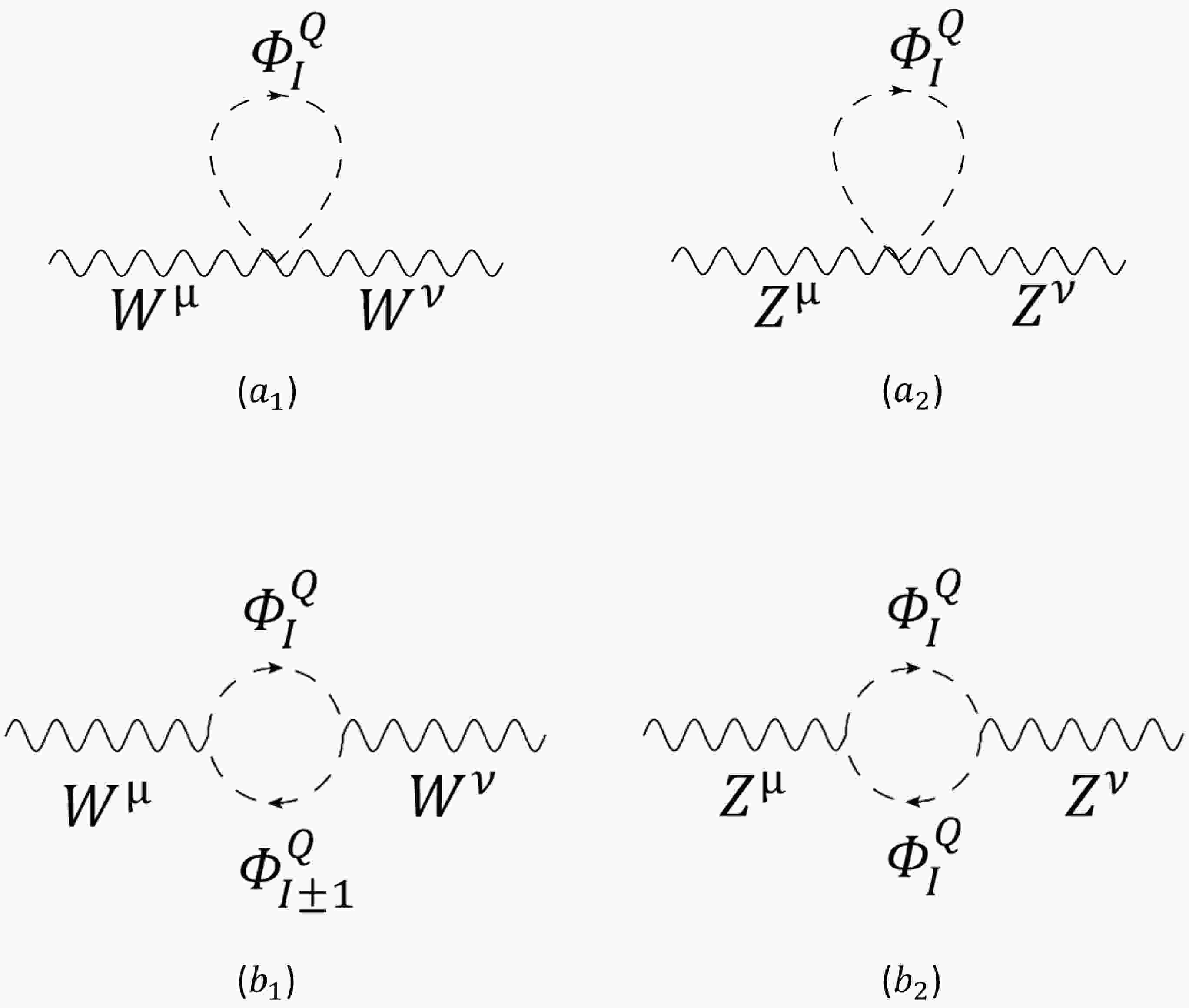
In the present model, the scalar multiplet would induce additional contributions to the W-boson mass by correcting the parameters T and S. As mentioned above, the associated corrections to these oblique parameters can be obtained by calculating the relevant Feynman diagrams shown in Figs. 1 and 2 for various vacuum polarization tensors of EW gauge bosons. As a result, the contribution of the scalar multiplet
$ \Phi_{JY} $ to T is given by
Figure 1. One-loop Feynman diagrams for the
$ WW $ and$ ZZ $ vacuum polarization tensors, which can give the leading-order contribution to the T parameter. Diagrams$ (a_{1,2}) $ involve only one internal scalar line, whereas the loops in diagrams$ (b_{1,2}) $ are enclosed by two scalar lines.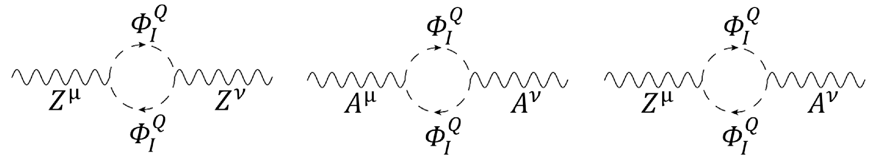
Figure 2. One-loop Feynman diagrams for the
$ ZZ $ ,$ AA $ , and$ ZA $ vacuum polarization tensors that contribute to the S parameter.$ \begin{equation} T_{\Phi_{JY}}=\frac{1}{4\pi s_{w}^{2}m_{W}^{2}}\sum\limits_{I=-J}^{J-1}N_{I+1}^{2}F\left(m_{\varPhi_{I}^{Q}}^{2},m_{\varPhi_{I+1}^{Q}}^{2}\right)\,, \end{equation} $

(14) where the function
$ F(A,B) $ is defined in Eq. (37) in Appendix C, while the correction of$ \Phi_{JY} $ to S is provided as follows:$ \begin{equation} S_{\Phi_{JY}}=-\frac{Y}{3\pi}\sum\limits_{I=-J}^{J}I\ln m_{\varPhi_{I}^{Q}}^{2}\,. \end{equation} $

(15) In this study, we rederive the above scalar contributions to T and S independently with the details given in Appendix D, for which we use the Feynman integrals and functions listed in Appendix C. The final expressions confirm the results in literature [134, 175, 176].
According to Eqs. (14) and (15), mass differences among components in the additional scalar multiplet
$ \Phi_{JY} $ are necessary to generate nonzero contributions to the oblique parameters T and S, which is required to explain the W-mass anomaly. Note that mass splitting can only be generated in the scalar potential of Eq. (9) via the following term:$ \begin{eqnarray} O_{4}=\lambda_{4}\left(\Phi_{JY}^{\dagger}T_{\Phi_{JY}}^{a}\Phi_{JY}\right)\left(H^{\dagger}T_{H}^{a}H\right)\,. \end{eqnarray} $

(16) Consequently, we focus on this term in our discussions on specific models. Furthermore, note that
$ O_4 $ is also constrained by perturbativity via$ |\lambda_4| < 4\pi $ as a dimensionless coupling [177]. In the following discussion, we take$ |\lambda_4| \leq 10 $ as the perturbative limit. -
With the general expression of the one-loop correction to the W-boson mass in Eq. (11) and the associated formulae for the oblique parameters T and S in Eqs. (14) and (15), we study several specific models of phenomenological interest, which are classified by the
$S U(2)_L$ representations J and hypercharges Y of the introduced scalar$ \Phi_{JY} $ . -
First, we consider the scalar multiplet to be in a real representation under the weak isospin
$S U(2)_L$ group with$ Y=0 $ . According to the definition, a real$S U(2)_{L}$ multiplet is related to its complex conjugate as follows:$ \begin{equation} \epsilon_{mm^{'}}...\epsilon_{cc^{'}}\epsilon_{bb^{'}}\epsilon_{aa^{'}}\left(\Phi^{*}\right)^{a^{'}b^{'}c^{'}...m^{'}}=\Phi_{abc...m}\,, \end{equation} $

(17) where the Latin indices with the values of 0 or 1 denote those under the
$S U(2)_L$ fundamental representation and$ \begin{equation} \epsilon_{ab}=\left(\begin{array}{cc} 0 & -1\\ 1 & 0 \end{array}\right). \end{equation} $

(18) We can also write the multiplet in terms of its components as
$ \begin{equation} \Phi_{JY}=\frac{1}{\sqrt{2}}\left(\begin{array}{c} ......\\ \varPhi_{I}^{Q}\\ ...... \end{array}\right)\,. \end{equation} $

(19) Thus, the transformation in Eq. (17) can be expressed by
$ \begin{equation} \left(\varPhi_{I}^{Q}\right)^{*}=\varPhi_{-I}^{Q}\,. \end{equation} $

(20) After EW symmetry breaking, the SM Higgs doublet obtains its VEV and can be written in the unitary gauge as
$ \begin{equation} H=\left(\begin{array}{c} 0\\ \dfrac{v+h}{\sqrt{2}} \end{array}\right)\,. \end{equation} $

(21) Then, we have
$ \begin{aligned}[b] O_{4}=&\lambda_{4}\left(\Phi_{JY}^{\dagger}T_{\Phi_{JY}}^{a}\Phi_{JY}\right)\left(H^{\dagger}T_{H}^{a}H\right)\\ =&\lambda_{4}\left(\Phi_{JY}^{\dagger}T_{\Phi_{JY}}^+\Phi_{JY}\right)\left(H^{\dagger}T_{H}^-H\right)\\&+\lambda_{4}\left(\Phi_{JY}^{\dagger}T_{\Phi_{JY}}^-\Phi_{JY}\right)\left(H^{\dagger}T_{H}^+H\right)\\ &+\lambda_{4}\left(\Phi_{JY}^{\dagger}T_{\Phi_{JY}}^{3}\Phi_{JY}\right)\left(H^{\dagger}T_{H}^{3}H\right)\\ =&-\frac{\lambda_{4}}{4}\left(h+v\right)^{2}\sum\limits_{I=-J}^{J}I\varPhi_{I}^{Q}\left(\varPhi_{I}^{Q}\right)^{*}\\ \supset&-\frac{\lambda_{4}}{4}v^{2}\sum\limits_{I=-J}^{J}I\varPhi_{I}^{Q}\left(\varPhi_{I}^{Q}\right)^{*}\,, \end{aligned} $

(22) where the term on the right-hand side of the last relation gives rise to mass splitting among the scalar components from
$ O_4 $ . However, according to Eq. (20), we have$ \begin{equation} \varPhi_{I}^{Q}\left(\varPhi_{I}^{Q}\right)^{*}=\varPhi_{-I}^{Q}\left(\varPhi_{-I}^{Q}\right)^{*}, \end{equation} $

(23) which leads to the following relations:
$ \begin{align} \begin{cases} -\dfrac{\lambda_{4}}{4}v^{2}\left[I\varPhi_{I}^{Q}\left(\varPhi_{I}^{Q}\right)^{*}-I\varPhi_{-I}^{Q}\left(\varPhi_{-I}^{Q}\right)^{*}\right]=0, & I > 0,\\ -\dfrac{\lambda_{4}}{4}v^{2}I\varPhi_{I}^{Q}\left(\varPhi_{I}^{Q}\right)^{*}=0, & I=0\,. \end{cases} \end{align} $

(24) According to Eq. (24), for any integer J, all the mass terms for
$ I\neq0 $ are canceled out while the$ I=0 $ mass term vanishes. Consequently, the$ O_{4} $ term does not contribute to the mass splittings among scalars in the real multiplet. In light of Eqs. (14) and (15), this model with a real multiplet cannot account for the W-boson mass anomaly at the one-loop level owing to the vanishing values of T and S.Note that the case with a real scalar multiplet without its VEV is usually regarded as a natural DM candidate [141, 142] because the neutral component can be the lightest owing to the one-loop mass corrections. The result shows that minimal scalar DM cannot provide us with a viable solution to the W-mass anomaly.
-
For a complex multiplet, Eq. (22) shows that each component in the scalar multiplet can obtain the following mass correction from
$ O_{4} $ $ \begin{equation} -\frac{\lambda_{4}}{4}v^{2}\sum\limits_{I=-J}^{J}I\varPhi_{I}^{Q}\left(\varPhi_{I}^{Q}\right)^{*}\,. \end{equation} $

(25) Because
$ \Phi_{JY} $ is complex, we have$ \begin{equation} \left(\varPhi_{I}^{Q}\right)^{*}\neq\varPhi_{-I}^{Q}\,, \end{equation} $

(26) so that
$ O_4 $ will induce an equal mass splitting between the adjacent components of$ \Phi_{JY} $ . Consequently, a complex scalar multiplet will make a contribution to the W-boson mass.In light of Eq. (15), the scalar multiplet
$ \Phi_{JY} $ does not contribute to S in the case of$ Y=0 $ . Thus, the W-boson mass is expressed only by T as$ \begin{equation} M_{W}=M_{W,SM}\left(1+\frac{\alpha\left(M_{Z}^{2}\right)c_{W}^{2}}{2\left(c_{W}^{2}-s_{W}^{2}\right)}T\right). \end{equation} $

(27) Figure 3 illustrates the parameter spaces in the cases with
$ Y=0 $ and$ J= $ 1/2, 1, 2, 3. The horizontal axis labeled as$ M_{L} $ represents the mass of the lightest particle in the multiplet in the range from 300 GeV to 3000 GeV, and the vertical axis denotes the mass difference between adjacent components. In each plot, the yellow shaded area shows the parameter space allowed by the EW global fit for T in the$ 2 \sigma $ C.L. range when$ S=U=0 $ , which is obtained from Ref. [41], while the solid blue region corresponds to the$ 2\sigma $ range of the W-boson mass measured by$ {\rm CDF\rm{-}II} $ . The red line represents the perturbative upper limit of$ | \lambda_{4} | \lesssim 10 $ , which can be directly related to the mass splittings of the scalar multiplet according to Eq. (25). As a result, there is always an overlap of the yellow and blue regions, meaning that most parameters explaining the$ M_W $ anomaly are consistent with the EW precision tests in models with a scalar multiplet of$ Y=0 $ , no matter the value of J. However, the required mass difference inside the mutiplet decreases with the increase in J, and hence, the perturbative limit becomes looser. In particular, the perturbativity imposes strong constraints on the lightest scalar mass, making it smaller than$ \sim 900\; (1800) $ GeV when the weak isospin is chosen to be$ J=1/2\; (1) $ . We can also plot the parameter spaces in the$ M_L $ -J plane, as shown in Fig. 4. With the same mass difference, the lightest mass$ M_L $ in the scalar multiplet is positively correlated with its value of J. Moreover, with the increase in the mass splitting$ \sqrt{\Delta M^2} $ , the scalar mass tends to be larger with a fixed J. In summary, according to Figs. 3 and 4, there are sufficient parameter spaces for a model with an extra complex scalar multiplet of$ Y=0 $ to explain the W-boson mass excess without disturbing the relevant experimental and theoretical bounds.
Figure 3. (color online) Parameter spaces in the
$ M_{L} $ -$ \sqrt{|\Delta M^{2}|} $ plane for models with complex scalar multiplets with$ Y=0 $ and$ J= $ 1/2, 1, 2, 3. The horizontal axis represents the mass of the lightest particle in the multiplet ($ M_{L} $ ) {in the range from 300 GeV to 3000 GeV}, and the vertical axis represents the mass difference between adjacent components. The yellow part is the parameter space allowed by electroweak global fit for T in the$ 2 \sigma $ C.L. range when$ S=U=0 $ , which is obtained from the electroweak global fit in Ref. [41]. The solid blue area is the parameter space that can explain the W mass measured by$ {\rm CDF\rm{-}II} $ in the$ 2 \sigma $ C.L. range, and the yellow shadow area is the parameter space meeting the requirements. The red solid line is the corresponding mass difference with$ | \lambda_{4} |=10 $ , and the area below the red line is consistent with perturbativity.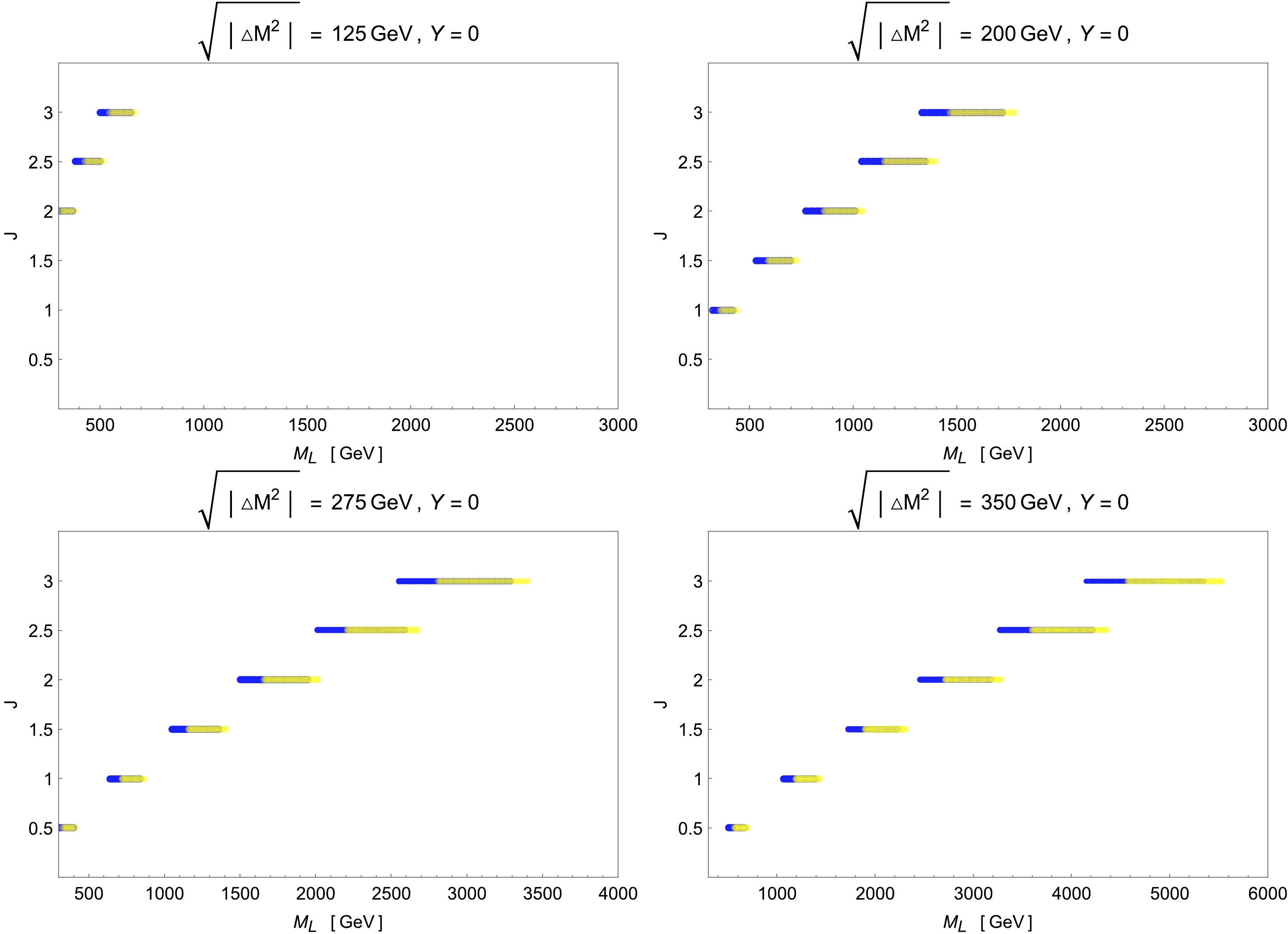
Figure 4. (color online) Parameter spaces in the
$ M_{L} $ -J plane for models with scalar multiplets of$ Y=0 $ and$ \sqrt{|\Delta M^{2}|}= $ 125, 200, 275, and 350 GeV for$ \lambda_{4}=1 $ , 2.6, 5, and 8, respectively. The color codings are the same as in Fig. 3, where all the plots satisfy the pertubative limit as shown by the values of$ \lambda_4 $ . -
In this subsection, we pay attention to the models in which a complex scalar multiplet with
$ Y=J $ ($ J \geq 1/2 $ ) is included in the particle spectrum. In such models, mass differences among scalars also arise from the operator$ O_4 $ , as in Eq. (25). Depending on the sign of$ \lambda_4 $ , the models can be divided into two types:Type A: If
$ \lambda_4 >0 $ , the lightest particle is the most charged in the multiplet with$ M_L = M_C $ , where$ M_L $ denotes the mass of the lightest scalar in$ \Phi_{JY} $ , and$ M_C $ is the mass of the most electrically charged particle. By taking the case with$ J=Y=2 $ as an example, the mass ordering is$ M_{\Phi^0} > M_{\Phi^+} > M_{\Phi^{++}}> M_{\Phi^{+++}}> M_{\Phi^{++++}} \equiv M_C $ , where we denote the corresponding components by their electric charges.Type B: If
$ \lambda_4<0 $ , the lightest scalar is the electrically neutral one in the multiplet with$ M_L = M_0 $ , where$ M_0 $ denotes the mass of the neutral component. In this case, by setting$ J=Y=2 $ , the component masses are ordered as$ M_{\Phi^{++++}}> M_{\Phi^{+++}} > M_{\Phi^{++}} > M_{\Phi^+} > M_{\Phi^0} \equiv M_0 $ . With mass splittings among the scalars in the multiplet, Eq. (11) shows that the model can potentially explain the W-mass anomaly with nonzero corrections to the parameters T and S while fixing$ U=0 $ .Figures 5 and 6 show the parameter spaces in the
$ M_W $ -$ \sqrt{\Delta m^2} $ plane for the Type-A and Type-B models by setting$ Y=J= 1/2 $ , 1, 2, and 3. The color codings are the same as those in Fig. 3, except the$ 2\sigma $ CL constraints on the oblique parameters T and S in this case are obtained using the EW global fits illustrated as the red ellipsis in Fig. 1 of Ref. [92]. It turns out that for all Type-A models of physical interest, there are always ample available parameter spaces to solve the CDF-II$ M_W $ anomaly while being allowed by the EW global fits and perturbativity. Moreover, for$ J=Y= 1/2\; (1) $ , the validity of the perturbative calculations limits the mass of the lightest scalar component as$ M_L \lesssim 900\; (\lesssim 1500) $ GeV, whereas when$ J=Y\geq 2 $ , the perturbativity does not provide any useful constraints owing to the decrease in the required mass differences. However, as shown in Fig. 6, the situation changes greatly for Type-B models. In this case, the CDF-II regions used to explain the$ M_W $ excess are entirely excluded by the global fits of various EW precision observables for all models with$ J=Y\geq 2 $ . For the scalar triplet with$ J=Y=1 $ , compared with its Type-A counterpart, the low-mass region with$ M_L\lesssim 700 $ GeV and the high-mass region with$ M_L \gtrsim 1800 $ GeV are disfavored by the EW global fits and perturbativity, respectively. Finally, constrained by the perturbativity upper bound on$ \lambda_4 $ , the model with an EW doublet of$ J=Y= $ 1/2 now admits the parameter space with$ M_L \lesssim 900 $ GeV to account for the$ M_W $ signal observed by CDF-II.
Figure 5. (color online) Parameter spaces in the
$ M_{L}-\sqrt{|\Delta M^{2}|} $ plane for Type-A models with scalar multiplets of$ Y=J= $ 1/2, 1, 2, and 3. In this type of model, the lightest scalar is the most charged, that is,$ M_{L}=M_{C} $ . The color codings are the same as in Fig. 3, except that the yellow area in each plot is obtained via the EW global fits of T and S, as illustrated by the red ellipsis in Fig. 1 of Ref. [92].
Figure 6. (color online) Legend is the same as in Fig. 5 but for Type-B models.
-
In light of Secs. III B and III C, we find that the value of Y might have a significant influence on the scalar multiplet explanation of the CDF-II
$ M_W $ anomaly. For the sake of comprehensiveness, we now investigate the effects of varying Y on the allowed parameter space. To be concrete, we consider the model that includes an extra scalar multiplet with$ J=2 $ ,$ \lambda_4>0 $ and$ Y=\pm 1/2 $ ,$ \pm 1 $ ,$ \pm 2 $ , and$ \pm 5 $ . As shown below, with$ \lambda_4 >0 $ , the phenomenology of models with positive Y is different from that with negative Y; hence, we show these two cases separately in Figs. 7 and 8, respectively. The color codings in these two plots are the same as in Fig. 3.
Figure 7. (color online) Legend is the same as in Fig. 5 but for models with an additional scalar multiplet of
$ J=2 $ and$ Y= 1/2 $ , 1, 2, and 5.
Figure 8. (color online) Legend is the same as in Fig. 5 but for models with an additional scalar multiplet of
$ J=2 $ and$ Y= -1/2 $ , -1, -2, and -5.From Fig. 7, we find that the mass splitting between two neighboring components required to solve the W-mass anomaly increases gradually with increasing Y in all ranges of
$ M_L $ . Moreover, in all cases, most parameter spaces explaining the$ M_W $ excess can be accommodated by the EW global fits, except the low-mass regions with$ M_L \lesssim 300\; (800) $ GeV for benchmarks with$ Y=2\; (5) $ . Furthermore, the upper limit from the perturbativity of$ \lambda_4 $ only gives a relevant constraint on parameter regions with large values of$ M_L $ . In particular, the perturbative limit rules out the portion with$ M_L \gtrsim 2900\; (2500) $ GeV for the multiplet with$ Y=2\; (5) $ .In contrast, as shown in Fig. 8, the parameter spaces allowed by all experimental data are greatly reduced when Y becomes more negative, especially for low
$ M_L $ regions. Furthermore, all blue bands in the cases of$ Y \leqslant -2 $ , which explain the CDF-II measured values of$ M_W $ , are now entirely excluded by the EW precision data. From our working experience, the experimental limit of the oblique parameter S gives the dominant constraint to models with negative Y'. We can understand this result by inspecting the expression of S in the limit of small mass splittings from$ O_4 $ as follows:$ \begin{aligned}[b] S =&-\frac{Y}{3\pi}\left(2\ln M_{\varPhi_{2}}^{2}+\ln M_{\varPhi_{1}}^{2}-\ln M_{\varPhi_{-1}}^{2}-2\ln M_{\varPhi_{-2}}^{2}\right) \\ =&-\frac{Y}{3\pi}\left[2\ln\left(\frac{M_{\varPhi_{-2}}^{2}-\lambda_{4}v^{2}}{M_{\varPhi_{-2}}^{2}}\right)+\ln\left(\frac{M_{\varPhi_{-1}}^{2}-\lambda_{4}v^2/2 }{M_{\varPhi_{-1}}^{2}}\right)\right] \\ \approx & \frac{\lambda_{4}Y}{3\pi}\left(\frac{2v^{2}}{ M_{\varPhi_{-2}}^{2}}+\frac{v^{2}}{2 M_{\varPhi_{-1}}^{2}}\right)\,, \end{aligned} $

(28) where the subscript I of the scalar
$ \Phi_I $ denotes the third isospin value of the component whose electric charge can be obtained by$ Q=I+Y $ . The last relation is the approximation when$ |\lambda_4 v^2| \ll M_{\Phi_I} $ for any I. It is shown from Eq. (28) that for$ \lambda_4 >0 $ , a negative value of Y leads to$ S < 0 $ . According to the EW global fit shown by the red circle in Fig. 1 in Ref. [92], the current EW precision data together with the new CDF-II measurement of$ M_W $ constrained$ -0.04 \lesssim S \lesssim 0.36 $ at the 2σ CL. This means that a multiplet scalar with$ Y < 0 $ would suffer from a significantly stronger constraint of S than that with$ Y>0 $ , which explains the differences shown in Figs. 7 and 8.Finally, we conclude this section by mentioning that the EW global fit constraints we apply here from Refs. [41,92] already included the latest CDF-II W-mass measurement in their calculations of the allowed
$ 2\sigma $ fit regions; therefore, the presentations of the CDF-II W-mass 2σ CL range in Figs. 3–8 do not, in principle, provide any independent information. However, we still regard it valuable to show the CDF-II W-mass-only bands because they illustrate the degree of difficulty in making this new W-mass measurement compatible with other EW global fit variables within the present models with extended scalar sectors. This is clearly observed, in particular, in Figs. 6 and 8, in which there are CDF-II preferred regions not allowed by the global fit data. Therefore, we keep the CDF-II signal region in all plots in this section. -
In light of the recent measurement of the W-boson mass by the CDF-II Collaboration, we comprehensively explain this
$ M_W $ anomaly in terms of the one-loop effects of a general$S U(2)_{L}$ scalar multiplet. As shown in literature, in the case without scalar VEVs, the dominant contribution to$ M_W $ can be expressed at leading order as the linear combination of the oblique parameters T and S, which is constrained by the global fits of various EW precision observables. Moreover, the operator$ O_4 $ gives rise to the main contribution to the mass splittings among components in the multiplet, which is needed to generate nonzero corrections to T and S. Thus, its coefficient$ \lambda_4 $ would be limited by the perturbativity. In this study, we rederive the general formulae for the one-loop contributions to T and S from a scalar multiplet, confirming the results in literature. We apply these analytic expressions to several models to explore the effects of the multiplet isospin representations and hypercharges on the viability of explaining the CDF-II$ M_W $ anomaly. As a result, for a scalar under the$S U(2)_L$ real representation with$ Y=0 $ , the model cannot explain the$ M_W $ excess at the one-loop level because the mass splitting between adjacent scalar components vanishes. In contrast, the mass differences would be induced by$ O_4 $ for a general complex representation, and hence, such models would potentially solve the$ M_W $ discrepancy between SM calculations and CDF-II values. Concretely, for the mutliplets with$ Y=0 $ , the$ M_W $ excess can be explained solely by the corrections of T due to$ S = 0 $ . All models with$ J=1/2 $ , 1, 2, and 3 are shown to have sufficient parameter spaces to meet the$ {\rm CDF\rm{-}II} $ result and EW global fits. For the cases with$ Y=J $ , the phenomenology can be divided into two classes depending on the sign of$ \lambda_4 $ . If$ \lambda_4 > 0 $ , the models are labeled as Type-A, in which the lightest scalar is the most charged. It turns out that there are always parameter spaces that can accommodate the CDF-II$ M_W $ value while still agreeing with the EW global fits and perturbativity limit. Conversely, for the Type-B models with$ \lambda_4 < 0 $ , the lightest particle is the electrically neutral scalar. The parameter region simultaneously allowed by the CDF-II and EW precision test data shrinks greatly with increasing$ J=Y $ . In particular, when$ J=Y\geqslant 2 $ , all regions with the lightest scalar mass below 3000 GeV are ruled out by the EW precision tests. In addition, we investigate the effects of the hypercharge Y on the scalar multiplet solution to the$ M_W $ anomaly. We fix$ J=2 $ and take$ \lambda_4 >0 $ . When Y is positive, the parameter spaces always exist for the interpretation of the$ M_W $ excess while allowed by other constraints. However, for$ Y<0 $ , only the cases with$ -1 \leq Y<0 $ allow parameter spaces for a viable explanation of the W-boson mass anomaly, whereas for$ Y\leqslant -2 $ , all CDF-II favored regions are excluded by the constraint on the oblique parameter S.It was argued in Ref. [134] that when the multiplet scalar masses are light or the multiplet representation J is high, the oblique parameter U offers a sizable contribution to the W-boson mass. Concretely, for the high-multiplet cases with
$ J=2 $ and$ J=3 $ , we find that when the scalar particles are sufficiently light, for example, if the mass of the lightest particle is only$ M_L= $ 200 GeV, U will give a W mass correction as large as 10%–15% of that of T or S. Therefore, even though T and S still dominate over the$ M_W $ correction, the effect of U cannot be ignored. However, when$ M_L $ increases to above 500 GeV, the effect of U on$ M_W $ is significantly suppressed and only contributes to 1% of$ M_W $ corrections compared with the dominant T parameter. This result can be understood from the EFT perspective. The T and S parameters originate from dimension-6 operators, whereas U is from a dimension-8 operator. Only when we take a low cutoff scale, which can be identified as the lightest scalar mass,$ \Lambda \sim M_L \sim $ 200 GeV, the suppression from the energy cutoff is not significant, and there is an observable effect from U. Moreover, the effect of U is sensitive to the isospin representation J. We find that when J takes an extraordinary value of$ J=8 $ for$ M_L= $ 300 GeV, the contribution of U to$ M_W $ can be comparable to or even larger than that of T. Nevertheless, in the present study, the mass of the multiplet scalar is large and$ J\leq 3 $ is relatively small; hence, the contribution of U is always suppressed compared with those of T and S.Finally, we comment on the possible collider signatures for such scalar multiplet extensions of the SM. In particular, note that for a high-dimensional representation, the multiplet contains highly electrically charged states in the spectrum, which would give us spectacular collider signals at the LHC. We take an example with an extra scalar multiplet of
$ J=Y=2 $ , in which the electric charges of scalars can be as high as$ \pm 4 $ . Moreover, we focus on the case in which the mass of the lightest scalar is smaller than 1 TeV, so that it could be produced directly at the high-luminosity run of the LHC. As studied in Sec. III.C, the Type-B case, in which the lightest scalar is neutral, has been ruled out under the scrutiny of the EW precision tests. Thus, in what follows, we concentrate on Type-A models, in which the lightest state is the most charged, whose electric charge is$ \pm $ 4. In Fig. 9, we show that heavy scalars can be produced dominantly through Drell-Yan processes [178–180] via the mediation of EW gauge bosons, such as W, Z, and photons. To study the LHC signatures of the generated multi-charged scalars, we need to specify their decay products. Note that in the Lagrangian in Eq. (9), there is accidental$ Z_2 $ symmetry imposed on the high-dimensional scalar multiplet$ \Phi_{JY} $ , which causes the lightest particle to be stable against decaying. In the Type-A multiplet with$ J=Y=2 $ , the lightest scalar should be$ \Phi^{\pm \pm \pm \pm} $ . If this state were stable, it would become a charged DM candidate, which is not allowed by current cosmological and astronomical observations. Therefore, we are required to break this problematic$ Z_2 $ symmetry. There are two ways to achieve this. First,$ Z_2 $ symmetry can be broken spontaneously by allowing the neutral component to possess a small VEV$ v_\Phi $ . Even though$ v_\Phi $ would also give rise to new contributions to the W-boson mass at the tree level, the one-loop effects due to the modifications of T and S would still dominate over the$ M_W $ corrections as long as$ v_\Phi \lesssim 1 $ GeV, which is the region of an extra EW scalar VEV allowed by the EW global fits. As a result, the heavier states in the multiplet would first decay into the lightest one$ \Phi^{\pm \pm \pm \pm} $ via hierarchical cascades. In plot$ (a) $ of Fig. 10, we take, as an example, the cascade decay chain of the heaviest scalar$ \Phi^0 $ by emitting multiple W-bosons. With the VEV$ v_\Phi $ , the most charged scalar, which is also the lightest, would further decay into four W-bosons, as illustrated in plots$ (b) $ and$ (c) $ of Fig. 10. The other way to violate$ Z_2 $ symmetry is to add high-dimensional operators, such as the dimension-5 operator$ \Phi_{abcd}(H^{*})^{a}(H^{*})^{b}(H^{*})^{c}(H^{*})^{d} $ or the dimension-7 operator$ \Phi_{abcd}\left(\bar{L}^C\right)^{a}\left(\hat{L}\right)^{b}\left(\bar{L}^C\right)^{c}\left(\hat{L}\right)^{d} $ , where the capital letter C denotes the charge conjugation, whereas the lowercase Latin letters represent the fundamental$ S U(2)_L $ indices. As illustrated in plots$ (b) $ and$ (c) $ of Fig. 11, the above two operators would cause the lightest charged scalar$ \Phi^{\pm \pm \pm \pm} $ to decay into the final states with$ 4W+4\ell $ or$ 4W+4h $ , in which$ \ell $ and h denote the SM leptons and Higgs scalar, respectively. However, no matter which mechanism breaks the$ Z_2 $ symmetry, the decays of$ \Phi^{\pm \pm \pm \pm} $ would be greatly suppressed by either the small scalar VEV$ v_\Phi $ or the high multiplicity of the produced particles in the final states. Hence, a simple estimation shows that the lifetime of a four-charged scalar of$ {\cal O}(\rm TeV) $ should be of the order of several seconds. This means that this particle should be effectively stable at the LHC and only behave as a highly-charged state leaving tracks in the detectors [181–183] (also see, for example, Ref. [184] for a theoretical review as well as references therein). Because detailed discussions on the LHC signatures of the high-dimensional scalar multiplet are beyond the scope of this study, we leave them to future studies.
Figure 9. Dominant production channels for new scalar particles in the multiplet in the Type-A models with
$ J=Y=2 $ .
Figure 10. Decay chains of the scalar particles when the scalar multiplet has a VEV in the Type-A model with
$ J=Y=2 $ .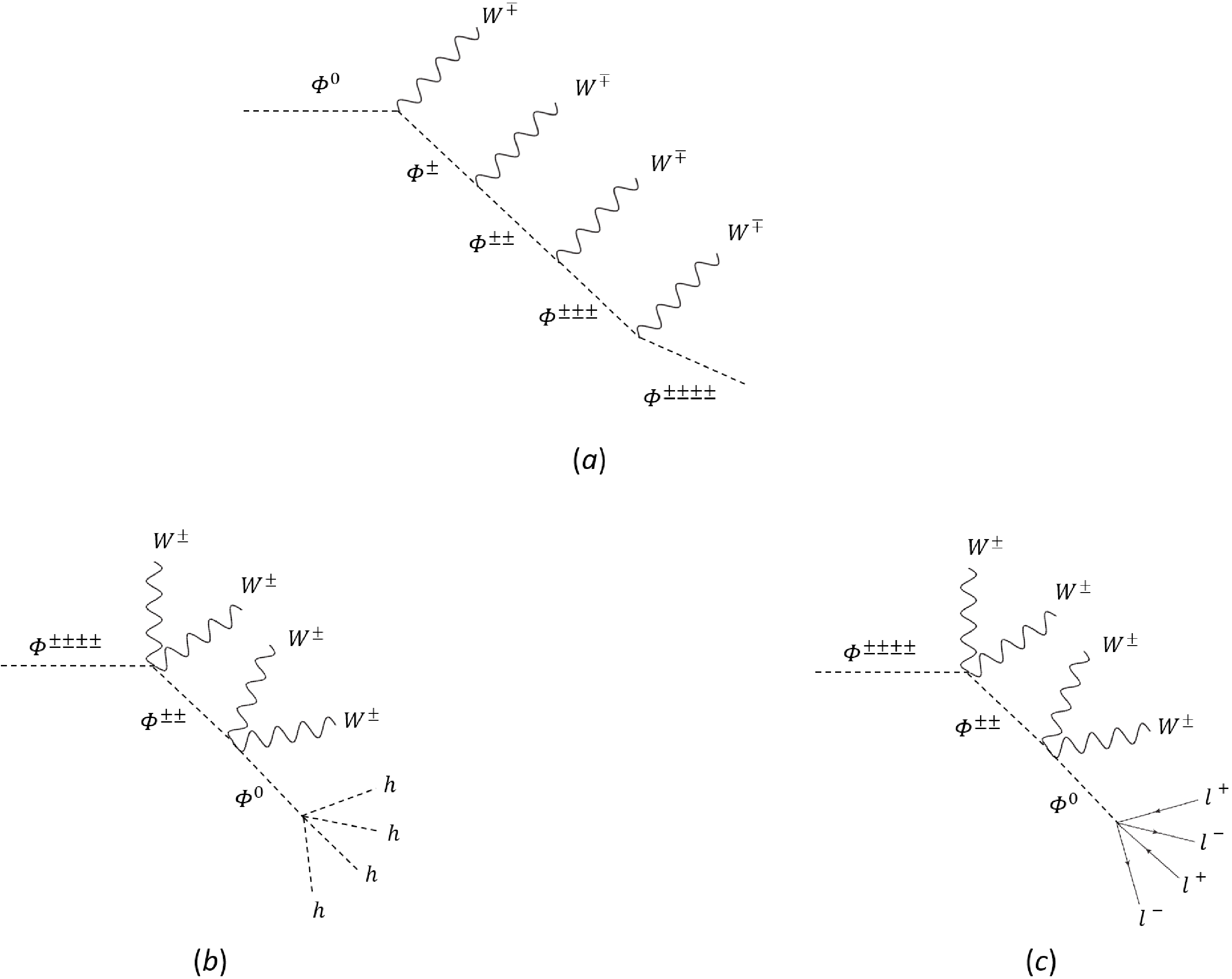
Figure 11. Decay chains of the scalar particles when the high-dimensional operators are introduced in the Type-A model with
$ J=Y=2 $ . -
In this appendix, we explicitly write the EW gauge couplings of a general scalar multiplet in the Lagrangian, which are useful in our calculation of the EW oblique parameters T and S. First, the weak neutral current part can be written as
$ \begin{aligned}[b] \mathcal{L}_{Z\Phi}& =\sum\limits_{I=-J}^{J}\partial_{\mu}\left(\varPhi_{I}^{Q}\right)^{*}\partial^{\mu}\varPhi_{I}^{Q}+\sum\limits_{I=-J}^{J}{\rm i}\frac{g}{c_{W}}\left(I-Qs_{W}^{2}\right)Z_{\mu}\left[\partial_{\mu}\left(\varPhi_{I}^{Q}\right)^{*}\varPhi_{I}^{Q}-\partial^{\mu}\varPhi_{I}^{Q}\left(\varPhi_{I}^{Q}\right)^{*}\right]\\ &+\sum\limits_{I=-J}^{J}\frac{g^{2}}{c_{W}^{2}}\left(I-Qs_{W}^{2}\right)^{2}Z_{\mu}Z^{\mu}\varPhi_{I}^{Q}\left(\varPhi_{I}^{Q}\right)^{*}\,,\\ \end{aligned} \tag{A1} $ 
and the weak charged current part is given by
$ \begin{aligned}[b] \mathcal{L}_{W\Phi}= &\sum\limits_{I=-J}^{J}\partial_{\mu}\left(\varPhi_{I}^{Q}\right)^{*}\partial^{\mu}\varPhi_{I}^{Q}\sum\limits_{I=-J}^{J}{\rm i}gW_{\mu}^+\left[N_{I}\varPhi_{I-1}^{Q}\partial_{\mu}\left(\varPhi_{I}^{Q}\right)^{*}-N_{I+1}\left(\varPhi_{I+1}^{Q}\right)^{*}\partial^{\mu}\varPhi_{I}^{Q}\right]\\ & +\sum\limits_{I=-J}^{J}{\rm i}gW_{\mu}^-\left[N_{I+1}\varPhi_{I+1}^{Q}\partial_{\mu}\left(\varPhi_{I}^{Q}\right)^{*}-N_{I}\left(\varPhi_{I-1}^{Q}\right)^{*}\partial_{\mu}\varPhi_{I}^{Q}\right]\\& +\sum\limits_{I=-J}^{J}g^{2}N_{I+1}^{2}W_{\mu}^+W_{\mu}^-\left(\varPhi_{I+1}^{Q}\right)^{*}\varPhi_{I+1}^{Q} +\sum\limits_{I=-J}^{J}g^{2}N_{I}^{2}W_{\mu}^+W_{\mu}^-\left(\varPhi_{I-1}^{Q}\right)^{*}\varPhi_{I-1}^{Q}\,, \end{aligned} \tag{A2}$

where the coefficient
$ N_I $ is defined below Eq. (7) in Sec. II.A. Finally, the interaction of scalar components with photons is written as$ \begin{aligned} \mathcal{L}_{A\Phi} =\sum\limits_{I=-J}^{J}\partial_{\mu}\left(\varPhi_{I}^{Q}\right)^{*}\partial^{\mu}\varPhi_{I}^{Q} +\sum\limits_{I=-J}^{J}{\rm i}eQA_{\mu}\left[\varPhi_{I}^{Q}\partial_{\mu}\left(\varPhi_{I}^{Q}\right)^{*}-\left(\varPhi_{I}^{Q}\right)^{*}\partial_{\mu}\varPhi_{I}^{Q}\right]\,. \end{aligned} \tag{A3} $

We can derive the Feynman rules for these EW gauge couplings from the Lagrangian, in which the three-point vertices are shown in Fig. A1 and the four-point ones are presented in Fig. A2.
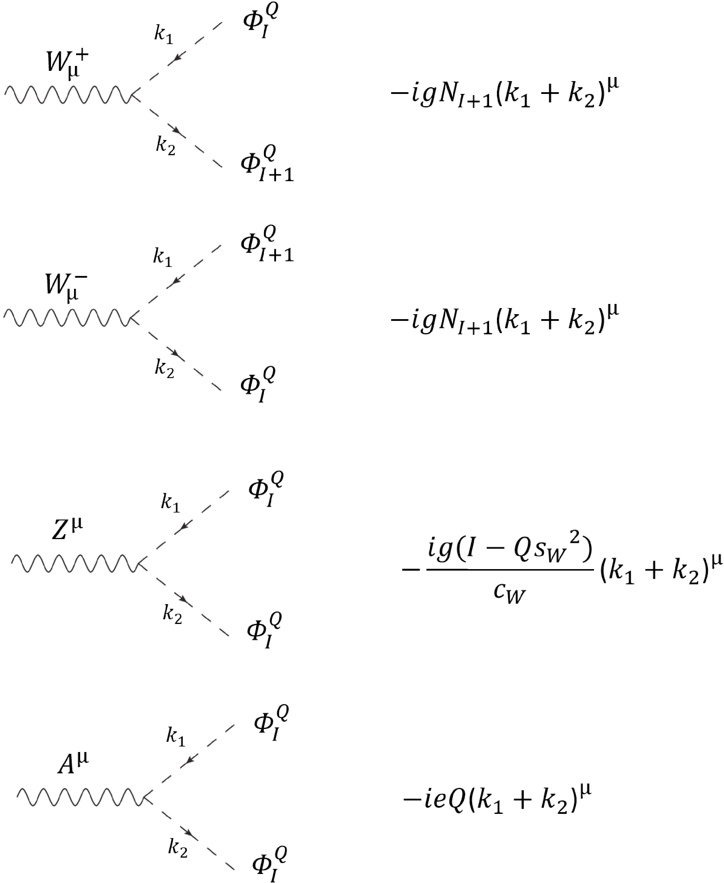
Figure A1. Three-point EW gauge couplings for components in a multiplet.
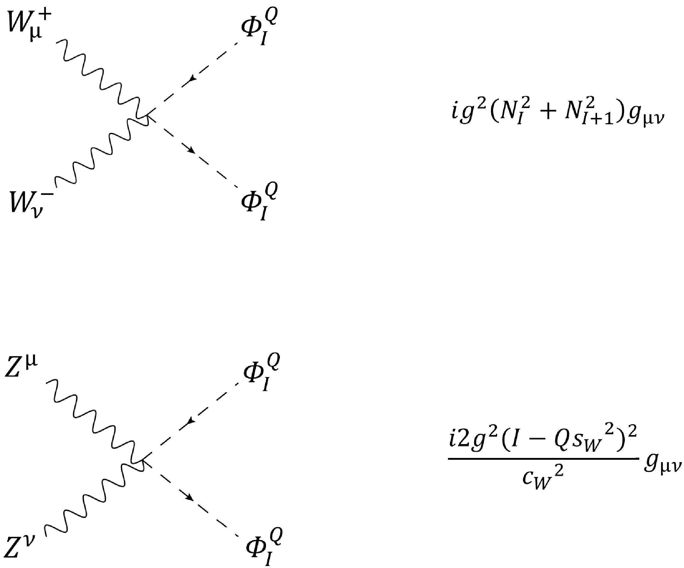
Figure A2. Four-point EW gauge couplings for components in a multiplet.
-
In this appendix, we show that the possible potential terms given in Eq. (10) can be written as linear combinations of other terms already existing in Eq. (9). We begin our discussion by expanding the operator
$ O_{6} $ in terms of scalar components in one multiplet as in Eq. (19):$ \begin{aligned}[b]\\[-8pt] O_6 =&\lambda_{6}\left(H^{\dagger}\Phi_{JY}\right)\left(\Phi_{JY}^{\dagger}H\right) =\lambda_{6}\sum\limits_{I=-J}^{J}C_{2J}^{J-I}\left[\left(H^{*}\right)^{a}\left(\varPhi_{I}\right)_{abc...m}\right]\left[\left(\varPhi_{I}^{*}\right)^{abc...m}H_{a}\right] \\ =&\lambda_{6}\sum\limits_{I=-J}^{J}C_{2J-1}^{J-I-1}\left[\left(H^{*}\right)^{0}\left(\varPhi_{I}\right)_{0}+\left(H^{*}\right)^{1}\left(\varPhi_{I}\right)_{1}\right]_{bc...m}\left[\left(\varPhi_{I}^{*}\right)^{0}H_{0}+\left(\varPhi_{I}^{*}\right)^{1}H_{1}\right]^{bc...m}\end{aligned} $ 
$ \begin{aligned}[b] =&\lambda_{6}\frac{\left(v+h\right)^{2}}{2}\sum\limits_{I=-J}^{J}C_{2J-1}^{J-I-1}\left(\varPhi_{I}\right)_{0bc...m}\left(\varPhi_{I}^{*}\right)^{0bc...m} =\lambda_{6}\frac{\left(v+h\right)^{2}}{2}\frac{C_{2J-1}^{J-I-1}}{C_{2J}^{J-I }}\varPhi_{I}^{Q}\left(\varPhi_{I}^{Q}\right)^{*} \\ =&\lambda_{6}\frac{\left(v+h\right)^{2}}{4}\sum\limits_{I=-J}^{J}\varPhi_{I}^{Q}\left(\varPhi_{I}^{Q}\right)^{*}-\frac{\lambda_{6}}{J}\frac{\left(v+h\right)^{2}}{4}\sum\limits_{I=-J}^{J}I\varPhi_{I}^{Q}\left(\varPhi_{I}^{Q}\right)^{*}, \end{aligned}\tag{B1} $

where
$ \left(H^{*}\right)^{1}=H_{1}=0 $ and$ \left(H^{*}\right)^{0}=H_{0}=\left(v+h\right)/\sqrt{2} $ in the unitary gauge. Moreover, we use another notation to represent the components in a multiplet,$ \left(\varPhi_{I}\right)_{abc...m}=\frac{1}{\sqrt{C_{2J}^{J-I}}}\varPhi_{I}^{Q}\,, \tag{B2} $

in which the lowercase Latin indices are those for the fundamental
$ S U(2)_L $ representation, and$ C^I_J \equiv J!/[I! (J-I)!] $ is the combinatorial number. According to Eq. (B1), the potential term$ O_{6} $ can be regarded as a linear combination of terms proportional to$ \lambda_{3} $ and$ \lambda_{4} $ . Therefore,$ O_{6} $ is not an independent operator. Similarly, we can prove that the term$ O_{7} $ does not represent a new interaction term either. -
When computing the oblique parameters T and S from scalar components, we encounter the below loop integrals. Because all these integrals are UV divergent, we apply dimensional regularization to obtain analytic expressions. For diagrams
$ (a_{1,2}) $ of Fig. 1, in which only one internal scalar propagator is involved, we must compute the loop integral [175] as follows:$ \mu^{4-d}\int\frac{d^{d}k}{\left(2\pi\right)^{d}}\frac{g^{\mu\nu}}{k^{2}-A+{\rm i}\varepsilon}=\frac{{\rm i}g^{\mu\nu}}{16\pi^{2}}A\left(div-\ln A\right)\,, \tag{C1} $

in which
$ div $ represents the UV divergent part given by$ div\equiv\frac{2}{4-d}-\gamma+1+\ln\left(4\pi\mu^{2}\right)\,, \tag{C2} $

where γ is Euler's constant, d is the spacetime dimensions, and μ is the sliding mass scale. However, diagrams
$ (b_{1,2}) $ in Fig. 1 can also give rise to contributions to the T parameter, in which the internal momentum integrals can be regularized as$ \begin{aligned}[b] &\mu^{4-d}\int\frac{d^{d}k}{\left(2\pi\right)^{\rm d}}\int_{0}^{1}{\rm d}x\frac{4k^{\mu}k^{\nu}}{\left[k^{2}-Ax-B\left(1-x\right)+{\rm i}\varepsilon\right]^{2}}\\ =&\frac{{\rm i}g^{\mu\nu}}{16\pi^{2}}\left[A\left(div-\ln A\right)+B\left(div-\ln B\right)+F\left(A,B\right)\right]\,, \end{aligned} \tag{C3} $

where x is the Feynman parameter, A and B denote the squared masses of the scalars in the loop, and the function
$ F(A,B) $ is defined by$ \begin{equation} F\left(A,B\right)\equiv\begin{cases} \dfrac{A+B}{2}-\dfrac{AB}{A-B}\ln\dfrac{A}{B}\,, & A\neq B\,,\\ 0\,, & A=B\,. \end{cases} \end{equation}\tag{C4} $

Moreover, to obtain the corrections to the oblique parameter S, we calculate the following integral for the Feynman diagrams in Fig. 2 [135]:
$ \begin{aligned}[b] & \left.\int_{0}^{1}{\rm d}x\frac{\partial}{\partial q}\left\{ \frac{4}{d}\mu^{4-d}\int\frac{d^{d}k}{\left(2\pi\right)^{d}}\frac{k^{2}}{\left[k^{2}-D\left(q,A,B,x\right)+{\rm i}\varepsilon\right]^{2}}\right\} \right|_{q=0}\\=&{\rm i}\left[div^{*}+\frac{K\left(A,B\right)}{48\pi^{2}}+\frac{\ln A+\ln B}{96\pi^{2}}\right]\,, \end{aligned}\tag{C5} $

where
$ D(q,A,B,x)\equiv q^{2}x(x-1)+Ax+B(1-x)\,, \tag{C6} $

with q representing the external four-momentum of gauge bosons,
$ \begin{aligned}[b]& K\left(A,B\right)\equiv\\&\begin{cases} -\dfrac{5}{6}+\dfrac{2AB}{\left(A-B\right)^{2}}+\dfrac{A^{3}+B^{3}-3AB\left(A+B\right)}{2\left(A-B\right)^{3}}\ln\dfrac{A}{B}\,, & A\neq B\,,\\ 0\,, & A=B, \end{cases} \end{aligned}\tag{C7} $

and
$ div^{*}=\frac{-1}{48\pi^{2}}\left[\frac{2}{4-d}-\gamma+\ln\left(4\pi\mu^{2}\right)\right]\,. \tag{C8} $

-
In this appendix, we rederive the analytic expressions for the one-loop contributions to the oblique parameters T and S from a general scalar multiplet. As mentioned in Sec. II.B, the expression of T is given by
$ T\equiv\frac{1}{\alpha m_{Z}^{2}}\left[\frac{A_{WW}\left(0\right)}{c_{W}^{2}}-A_{ZZ}\left(0\right)\right], \tag{D1} $

where
$ A_{VV^\prime}(q) $ is defined in terms of the vacuum polarization${\rm i}\Pi_{VV^\prime}^{\mu\nu}(q)$ as in Eq. (13). It turns out that the vacuum polarization of the W boson is given by$ \begin{aligned}[b]\\[-5pt] {\rm i}\Pi_{WW}^{\mu\nu}\left(0\right)=&\sum\limits_{I=-J}^{J}-g^{2}\left(N_{I}^{2}+N_{I+1}^{2}\right)\mu^{4-d}\int\frac{d^{d}k}{\left(2\pi\right)^{d}}\frac{g^{\mu\nu}}{k^{2}-m_{\varPhi_{I}^{Q}}^{2}+{\rm i}\varepsilon}\\ &+\sum\limits_{I=-J}^{J-1}g^{2}N_{I+1}^{2}\mu^{4-d}\int\frac{d^{d}k}{\left(2\pi\right)^{d}}\int_{0}^{1}{\rm d}x\frac{4k^{\mu}k^{\nu}}{\left[k^{2}-m_{\varPhi_{I}^{Q}}^{2}x-m_{\varPhi_{I-1}^{Q}}^{2}\left(1-x\right)+{\rm i}\varepsilon\right]^{2}}\\ &={\rm i}g^{\mu\nu}\sum\limits_{I=-J}^{J}\frac{-g^{2}\left(N_{I}^{2}+N_{I+1}^{2}\right)}{16\pi^{2}}m_{\varPhi_{I}^{Q}}^{2}\left(div-\ln m_{\varPhi_{I}^{Q}}^{2}\right)\\ &+{\rm i}g^{\mu\nu}\sum\limits_{I=-J}^{J-1}\frac{g^{2}N_{I+1}^{2}}{16\pi^{2}}\left[m_{\varPhi_{I}^{Q}}^{2}\left(div-\ln m_{\varPhi_{I}^{Q}}^{2}\right)+m_{\varPhi_{I+1}^{Q}}^{2}\left(div-\ln m_{\varPhi_{I+1}^{Q}}^{2}\right)\right.\left.+F\left(m_{\varPhi_{I}^{Q}}^{2},m_{\varPhi_{I+1}^{Q}}^{2}\right)\right]\,, \end{aligned} \tag{D2}$ 
so we can extract
$ A_{WW} $ as follows:$ \begin{aligned}[b] A_{WW}\left(0\right)=&\sum\limits_{I=-J}^{J}\frac{-g^{2}\left(N_{I}^{2}+N_{I+1}^{2}\right)}{16\pi^{2}}m_{\varPhi_{I}^{Q}}^{2}\left(div-\ln m_{\varPhi_{I}^{Q}}^{2}\right)+\sum\limits_{I=-J}^{J-1}\frac{g^{2}N_{I+1}^{2}}{16\pi^{2}}\left[m_{\varPhi_{I}^{Q}}^{2}\left(div-\ln m_{\varPhi_{I}^{Q}}^{2}\right)+m_{\varPhi_{I+1}^{Q}}^{2}\left(div-\ln m_{\varPhi_{I+1}^{Q}}^{2}\right)\right.\\ &\left.+F\left(m_{\varPhi_{I}^{Q}}^{2},m_{\varPhi_{I+1}^{Q}}^{2}\right)\right]=\frac{g^{2}}{16\pi^{2}}\sum\limits_{I=-J}^{J-1}N_{I+1}^{2}F\left(m_{\varPhi_{I}^{Q}}^{2},m_{\varPhi_{I+1}^{Q}}^{2}\right). \end{aligned}\tag{D3} $

The vacuum polarization of the Z boson is given by
$ \begin{aligned}[b] {\rm i}\Pi_{ZZ}^{\mu\nu}\left(0\right)=&\sum\limits_{I=-J}^{J}-\frac{2g^{2}\left(I-Qs_{W}^{2}\right)^{2}}{c_{W}^{2}}\mu^{4-d}\int\frac{d^{d}k}{\left(2\pi\right)^{d}}\frac{g^{\mu\nu}}{k^{2}-m_{\varPhi_{I}^{Q}}^{2}+{\rm i}\varepsilon}+\sum\limits_{I=-J}^{J}\frac{g^{2}\left(I-Qs_{W}^{2}\right)^{2}}{c_{W}^{2}}\mu^{4-d}\int\frac{d^{d}k}{\left(2\pi\right)^{d}}\int_{0}^{1}{\rm d}x\frac{4k^{\mu}k^{\nu}}{\left[k^{2}-m_{\varPhi_{I}^{Q}}^{2}+{\rm i}\varepsilon\right]^{2}}\\ =&{\rm i}g^{\mu\nu}\sum\limits_{I=-J}^{J}-\frac{2g^{2}\left(I-Qs_{W}^{2}\right)^{2}}{16\pi^{2}c_{W}^{2}}m_{\varPhi_{I}^{Q}}^{2}\left(div-\ln m_{\varPhi_{I}^{Q}}^{2}\right)+{\rm i}g^{\mu\nu}\sum\limits_{I=-J}^{J}\frac{2g^{2}\left(I-Qs_{W}^{2}\right)^{2}}{16\pi^{2}c_{W}^{2}}m_{\varPhi_{I}^{Q}}^{2}\left(div-\ln m_{\varPhi_{I}^{Q}}^{2}\right)\,,\\ \end{aligned} \tag{D4}$

so we have
$ A_{ZZ}\left(0\right)=\sum\limits_{I=-J}^{J}-\frac{2g^{2}\left(I-Qs_{W}^{2}\right)^{2}}{16\pi^{2}c_{W}^{2}}m_{\varPhi_{I}^{Q}}^{2}\left(div-\ln m_{\varPhi_{I}^{Q}}^{2}\right) +\sum\limits_{I=-J}^{J}\frac{2g^{2}\left(I-Qs_{W}^{2}\right)^{2}}{16\pi^{2}c_{W}^{2}}m_{\varPhi_{I}^{Q}}^{2}\left(div-\ln m_{\varPhi_{I}^{Q}}^{2}\right)=0\,. \tag{D5}$

Therefore, the contribution of the scalar multiplet
$ \Phi_{JY} $ to T is only provided by the$ A_{WW} $ part in Eq. (D1),$ T_{\Phi_{JY}}=\frac{g^{2}}{16\alpha\pi^{2}c_{w}^{2}m_{Z}^{2}}\sum\limits_{I=-J}^{J-1}N_{I+1}^{2}F\left(m_{\varPhi_{I}^{Q}}^{2},m_{\varPhi_{I+1}^{Q}}^{2}\right)=\frac{1}{4\pi s_{w}^{2}m_{W}^{2}}\sum\limits_{I=-J}^{J-1}N_{I+1}^{2}F\left(m_{\varPhi_{I}^{Q}}^{2},m_{\varPhi_{I+1}^{Q}}^{2}\right)\,. \tag{D6} $

In contrast, the expression for S is given by
$ S\equiv\frac{4s_{W}^{2}c_{W}^{2}}{\alpha}\left[A_{ZZ}^{\prime}\left(0\right)-\frac{c_{W}^{2}-s_{W}^{2}}{c_{W}s_{W}}A_{Z\gamma}^{\prime}\left(0\right)-A_{\gamma\gamma}^{\prime}\left(0\right)\right]\,, \tag{D7} $

where
$ A^\prime_{VV^\prime} $ is defined in Eq. (13) as the expansion of$ \Pi^{\mu\nu}_{VV^\prime} $ in terms of the external momentum q at the second order. First, we calculate the$ ZZ $ part:$ \begin{aligned}[b] A_{ZZ}^{\prime}\left(0\right) =&-{\rm i}\sum\limits_{I=-J}^{J}\frac{g^{2}\left(I-Qs_{W}^{2}\right)^{2}}{c_{W}^{2}}\left.\int_{0}^{1}{\rm d}x\frac{\partial}{\partial q}\left\{ \frac{4}{d}\mu^{4-d}\int\frac{d^{d}k}{\left(2\pi\right)^{d}}\frac{k^{2}}{\left[k^{2}-D\left(q,m_{\varPhi_{I}^{Q}}^{2},m_{\varPhi_{I}^{Q}}^{2},x\right)+{\rm i}\varepsilon\right]^{2}}\right\} \right|_{q=0}\\ =&\sum\limits_{I=-J}^{J}\frac{g^{2}\left(I-Qs_{W}^{2}\right)^{2}}{c_{W}^{2}}\left[div^{*}+\frac{K\left(m_{\varPhi_{I}^{Q}}^{2},m_{\varPhi_{I}^{Q}}^{2}\right)}{48\pi^{2}}+\frac{\ln m_{\varPhi_{I}^{Q}}^{2}}{48\pi^{2}}\right]=\sum\limits_{I=-J}^{J}\frac{g^{2}\left(I-Qs_{W}^{2}\right)^{2}}{c_{W}^{2}}\left(div^{*}+\frac{\ln m_{\varPhi_{I}^{Q}}^{2}}{48\pi^{2}}\right)\,, \end{aligned} \tag{D8} $

where
$ K\left(m_{\varPhi_{I}^{Q}}^{2},m_{\varPhi_{I}^{Q}}^{2}\right)=0\,, \tag{D9} $

based on Eq. (C7). Then, we calculate the
$ Z\gamma $ part:$ \begin{aligned}[b] A_{Z\gamma}^{\prime}\left(0\right) =&-{\rm i}\sum\limits_{I=-J}^{J}\frac{egQ\left(I-Qs_{W}^{2}\right)}{c_{W}}\left.\int_{0}^{1}{\rm d}x\frac{\partial}{\partial q}\left\{ \frac{4}{d}\mu^{4-d}\int\frac{d^{d}k}{\left(2\pi\right)^{d}}\frac{k^{2}}{\left[k^{2}-D\left(q,m_{\varPhi_{I}^{Q}}^{2},m_{\varPhi_{I}^{Q}}^{2},x\right)+{\rm i}\varepsilon\right]^{2}}\right\} \right|_{q=0}\\ =&\sum\limits_{I=-J}^{J}\frac{egQ\left(I-Qs_{W}^{2}\right)}{c_{W}}\left[div^{*}+\frac{K\left(m_{\varPhi_{I}^{Q}}^{2},m_{\varPhi_{I}^{Q}}^{2}\right)}{48\pi^{2}}+\frac{\ln m_{\varPhi_{I}^{Q}}^{2}}{48\pi^{2}}\right]=\sum\limits_{I=-J}^{J}\frac{egQ\left(I-Qs_{W}^{2}\right)}{c_{W}}\left(div^{*}+\frac{\ln m_{\varPhi_{I}^{Q}}^{2}}{48\pi^{2}}\right)\,. \end{aligned}\tag{D10} $

Finally, we calculate the
$ \gamma\gamma $ part:$ \begin{aligned}[b] A_{\gamma\gamma}^{\prime}\left(0\right) =&-{\rm i}\sum\limits_{I=-J}^{J}{\rm e}^{2}Q^{2}\left.\int_{0}^{1}{\rm d}x\frac{\partial}{\partial q}\left\{ \frac{4}{d}\mu^{4-d}\int\frac{d^{d}k}{\left(2\pi\right)^{d}}\frac{k^{2}}{\left[k^{2}-D\left(q,m_{\varPhi_{I}^{Q}}^{2},m_{\varPhi_{I}^{Q}}^{2},x\right)+{\rm i}\varepsilon\right]^{2}}\right\} \right|_{q=0}\\ =&\sum\limits_{I=-J}^{J}{\rm e}^{2}Q^{2}\left[div^{*}+\frac{K\left(m_{\varPhi_{I}^{Q}}^{2},m_{\varPhi_{I}^{Q}}^{2}\right)}{48\pi^{2}}+\frac{\ln m_{\varPhi_{I}^{Q}}^{2}}{48\pi^{2}}\right]=\sum\limits_{I=-J}^{J}{\rm e}^{2}Q^{2}\left(div^{*}+\frac{\ln m_{\varPhi_{I}^{Q}}^{2}}{48\pi^{2}}\right). \end{aligned}\tag{D11} $

Therefore, the contribution of a scalar multiplet
$ \Phi_{JY} $ to S is given by$ \begin{aligned}[b] S_{\Phi_{JY}}=&\sum\limits_{I=-J}^{J}\frac{4s_{W}^{2}c_{W}^{2}}{\alpha}\left\{\frac{g^{2}\left[I-\left(I+Y\right)s_{W}^{2}\right]^{2}}{c_{W}^{2}}-{\rm e}^{2}\left(I+Y\right)^{2}\right.\left.-\frac{eg\left(I+Y\right)\left(c_{W}^{2}-s_{W}^{2}\right)\left[I-\left(I+Y\right)s_{W}^{2}\right]}{c_{W}^{2}s_{W}}\right\}\left(div^{*}+\frac{\ln m_{\varPhi_{I}^{Q}}^{2}}{48\pi^{2}}\right)\\ =&-16\pi Y\sum\limits_{I=-J}^{J}I\left(div^{*}+\frac{\ln m_{\varPhi_{I}^{Q}}^{2}}{48\pi^{2}}\right)\,. \end{aligned} \tag{D12} $

Because the sum over the third isospin components I vanishes identically, that is,
$ Y\sum\limits_{I=-J}^{J}I=0\,,\tag{D13} $

the UV divergences in Eq. (D12) are canceled. Thus, the contribution of a scalar multiplet
$ \Phi_{JY} $ to S can be written as$ S_{\Phi_{JY}}=-\frac{Y}{3\pi}\sum\limits_{I=-J}^{J}I\ln m_{\varPhi_{I}^{Q}}^{2}. \tag{D14} $

Note that the expressions for
$ S_{\Phi_{JY}} $ and$ T_{\Phi_{JY}} $ are consistent with those given in Ref. [134].
W-boson mass anomaly from a general SU(2)L scalar multiplet
- Received Date: 2023-02-04
- Available Online: 2023-06-15
Abstract: We explain the W-boson mass anomaly by introducing an


 DownLoad: