


 Abstract
 HTML
HTML Reference
 Related
 PDF
PDF


-
Nuclei are complicated quantum many-body systems. According to quantum mechanics, the wave functions of low-lying nuclear states should be obtained by solving Schrödinger's equation. Practically, this is done by performing the full shell model calculation in a given model space. However, the configuration space can easily be huge in a large model space, which makes the full shell model calculation almost impossible. This difficulty motivates theorists to develop approximated shell model methods, so that the obtained nuclear wave functions are expected to be as close as possible to the exact shell model ones. Various approximated shell model methods, such as the shell model truncation [1], stochastic quantum Monte Carlo approaches and their extrapolations [2−5], the projected configuration interaction [6], the class of variation after projection (VAP) methods [7−12], and recent methods for shell model basis selection using the generator coordinate method (GCM) [13−15], have been developed. A relevant review can be found in Ref. [16].
Among these approximated shell model methods, the VAP is an important one, and it is believed to have a good shell model approximation in calculating low-lying states of nuclei [7−12]. Such an approximation can be continuously improved by adding more projected basis states to the calculated states. Certainly, the added projected states should be important so that the calculated states can be significantly improved. However, the problem is that, if an added projected state is randomly generated and does not mix with a calculated state at the beginning of the VAP iteration, it is likely that this added projected state will never mix with the state even after the VAP iteration converges. This means that such an added projected basis state is useless and must be abandoned. In this sense, a useful new projected state should mix with a calculated nuclear state at the beginning of the VAP iteration. Therefore, an effective way of obtaining new useful projected states before performing the VAP iteration is crucial in the VAP calculation.
This problem can be solved via previous methods, such as the Monte Carlo shell model (MCSM) [3]. In the MCSM, one selects the best new basis state from the stochastically generated candidates. To ensure the effectiveness of the new candidate, shell model Hamiltonian is diagonalized in a subspace spanned by all previously selected basis states and the candidate basis. One can then check the contribution of this candidate basis for reducing the energy eigenvalue being calculated. If the contribution is sufficient, this candidate basis will be added to the group of basis states. Otherwise, one needs to check the importance of the next basis candidate. After that, only important basis states are selected, and a good approximation is expected. However, in such basis selection, one may sometimes check a large amount of useless candidates before a new important basis is identified. Herein, we propose a new reliable and efficient algorithm that is completely different from the MCSM. In the proposed algorithm, a randomly generated useless projected state can be varied so that it may become a new important basis state for the VAP calculation.
The second problem in the VAP calculation is the poor orthonormality among the projected basis states, which seriously affects the accuracy of the calculated VAP wave functions and consequently reduces the stability of the VAP iteration. This problem was considered in our previous work [12], where the projected states were subjected to two constraints to prevent the appearance of redundant states throughout the VAP iteration. In the present work, we replace these two constraints with a new one, which is expected to be more efficient for keeping the projected basis states in good condition during the VAP calculation.
The remainder of this paper is organized as follows. Section II provides a solution for generating the useful projected basis states. Section III discusses the problem of orthonormality among the projected basis states. Section IV presents an example of the present VAP calculations. A brief summary and outlook are presented in Sec.V.
-
Let us first address the problem of the important projected basis states in the VAP calculation. We start with the simplified VAP wave function taken from our previous work [12]:
$ |\Psi^{(n)}_{J\pi M\alpha}(K)\rangle=\sum\limits_{i=1}^n f^{J\pi\alpha}_{i}P^{J\pi}_{MK}|\Phi_i\rangle, $

(1) where
$ |\Phi_i\rangle $ is a Slater determinant (SD) composed of deformed single-particle wave functions in the model space where the shell model calculation is performed.$ |\Phi_i\rangle $ has a good particle number but usually does not have a good spin and parity. Thus, the particle number projection can be omitted, but the angular momentum projection and parity projection should be applied in Eq. (1) so that$ |\Psi^{(n)}_{J\pi M\alpha}(K)\rangle $ has a good spin J and parity π. Here, we assume that all the adopted$ |\Phi_i\rangle $ SDs are fully symmetry-unrestricted. n represents the number of included$ |\Phi_i\rangle $ SDs.$ P_{M K}^{J\pi} $ represents the product of the angular momentum projection operator$ P_{M K}^{J} $ and the parity projection operator$ P^\pi $ . K can be randomly chosen in the range of$ |K|\leq J $ . α is used to differ the states with the same J, π, and M. The$ f^{J\pi\alpha}_{i} $ coefficients and the corresponding energy$ E^{(n)}_{J\pi\alpha} $ are determined via the Hill-Wheeler equation:$ \sum\limits_{i'=1}^{n}(H^{J\pi}_{ii'}-E^{(n)}_{J\pi\alpha}N^{J\pi}_{ii'})f_{i^{\prime}}^{J\pi\alpha}=0, $

(2) where
$ H_{i i'}^{J\pi}=\langle \Phi_i|\hat H P^{J\pi}_{KK}|\Phi_{i'}\rangle $ and$ N_{i i'}^{J\pi}=\langle \Phi_i|P^{J\pi}_{KK}|\Phi_{i'}\rangle $ . The normalization condition is imposed on the$ f^{J\pi\alpha}_{i} $ coefficients so that$ \langle\Psi^{(n)}_{J\pi M\alpha}(K)|\Psi^{(n)}_{J\pi M\alpha}(K)\rangle=1 $ . Here, we assume$ E^{(n)}_{J\pi 1}\leq E^{(n)}_{J\pi 2}\leq\cdots \leq E^{(n)}_{J\pi n} $ for a given n.In the present VAP, all the
$ |\Phi_i\rangle $ SDs in Eq. (1) are varied simultaneously, so that the$ E^{(n)}_{J\pi\alpha} $ energies and their corresponding$ |\Psi^{(n)}_{J\pi M\alpha}(K)\rangle $ wave functions obtained from Eq. (2) are as close as possible to the exact shell model ones. Details of our VAP algorithm can be found in Ref. [11].Naturally, one can directly take the trial wave function in Eq. (1) to perform the VAP iteration with the initial
$ |\Phi_i\rangle $ SDs randomly generated. As a simple example, we use the trial wave function in Eq. (1) with$ K = 0 $ to perform the VAP calculations for the ground$ 0^+ $ state in$ ^{64} $ Ge. The GXPF1A interaction [17] in the$ fp $ model space is taken. Thus, the parity projection can be omitted in this example. The results are shown in Fig. 1. It is seen that in the simplest case of$ n=1 $ , the VAP iteration converges quite fast, and the converged energy is$ -302.983 $ MeV. However, if one takes$ n=2 $ with random initial SDs, it is possible that the final converged VAP energy is also$ -302.983 $ MeV, which is the same as that with$ n=1 $ . This strongly implies that one of the two projected SDs does not contribute to the converged VAP wave function.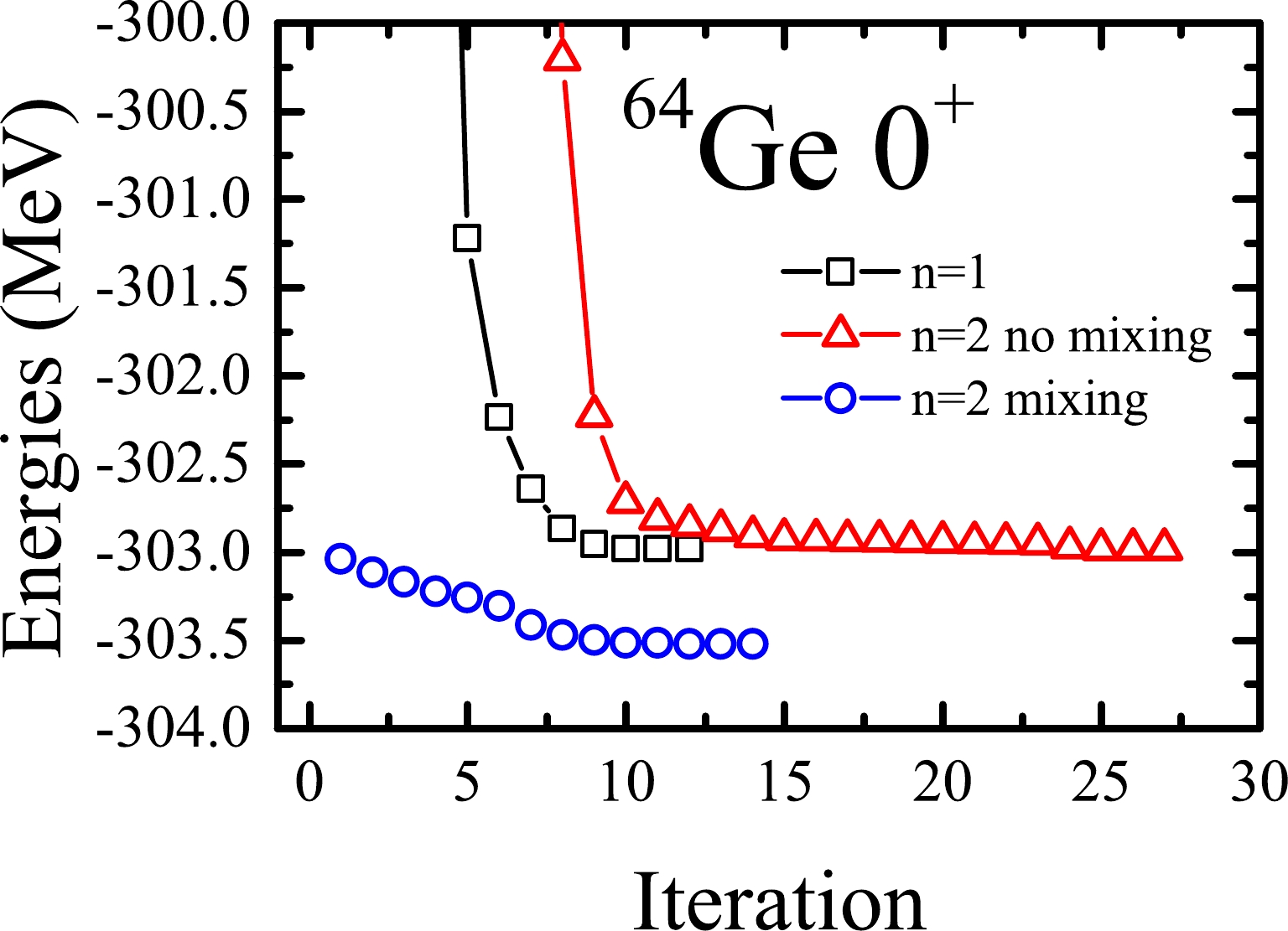
Figure 1. (color online) VAP iterations with n=1 (black square), n=2 without mixing (red triangle), and n=2 with mixing (blue circle) for
$ J^\pi=0^+ $ in$ ^{64} $ Ge.Let us try to understand why the above converged energy with
$ n=2 $ is exactly the same as that with$ n=1 $ . In the$ n=2 $ case, one can obtain two$ E^{(2)}_{J\pi\alpha} $ energies, and only the lower one ($ \alpha=1 $ ) is minimized. The corresponding$ \alpha=1 $ wave function can be explicitly written as$ \begin{array}{*{20}{l}} |\Psi^{(2)}_{J\pi M1}(K)\rangle=f^{J\pi 1}_{1}P^{J\pi}_{MK}|\Phi_1\rangle+f^{J\pi 1}_{2}P^{J\pi}_{MK}|\Phi_2\rangle. \end{array} $

(3) When the energy for Eq. (3) converges to
$ E^{(2)}_{J\pi 1}= -302.985 $ MeV (see red triangles in Fig. 1), it is found that the corresponding coefficients in Eq. (3) are$ f^{J\pi 1}_{1}= 11.2256 $ and$ f^{J\pi 1}_{2}=4.5315\times 10^{-8} $ . The latter$ f^{J\pi 1}_{2} $ is almost zero. This means that the second term in Eq. (3) is useless. Therefore, such VAP with$ n=2 $ is essentially the VAP with$ n=1 $ .Now, we need to understand why the second projected state in Eq. (3) cannot mix with the calculated wave function. Actually, during the VAP iteration, once the
$ f^{J\pi 1}_{2} $ is zero, the derivatives of the$ E^{(2)}_{J\pi 1} $ energy with respect to all the variational parameters (see the Appendix) for$ |\Phi_2\rangle $ must be zero. Consequently,$ |\Phi_2\rangle $ remains almost unchanged in the next VAP iteration, because the direction of the energy minimization should be close to the opposite direction of the energy gradient. Hence, it is likely that$ f^{J\pi 1}_{2} $ remains zero at the next iteration. Therefore, the second term in Eq. (3) becomes a complete bystander. Certainly, this situation must be avoided in practical calculations.One may wonder under what condition the second projected state can mix with the calculated wave function. We address this issue from a theoretical point of view.
If there is a new state
$ |\phi\rangle $ that does not mix with a known wave function$ |\psi\rangle $ , one can easily prove the following identity:$ \begin{array}{*{20}{l}} \langle \phi|(\hat H-E)|\psi\rangle=0, \end{array} $

(4) where
$ E=\langle\psi|\hat H|\psi\rangle $ . Here is a brief proof of Eq. (4). Actually,$ |\phi\rangle $ is usually not orthogonal to$ |\psi\rangle $ . Thus,$ |\phi\rangle $ needs to be orthogonalized by performing Gram-Schmidt orthogonalization, and the orthogonalized one can be written as$ \begin{array}{*{20}{l}} |\phi'\rangle=|\phi\rangle-\langle\psi|\phi\rangle|\psi\rangle, \end{array} $

(5) so that
$ \langle\psi|\phi'\rangle=0 $ . If there is no mixing between$ |\phi\rangle $ and$ |\psi\rangle $ , one should have$ \begin{array}{*{20}{l}} \langle \phi'|\hat H|\psi\rangle=0. \end{array} $

(6) By substituting Eq. (5) into Eq. (6), one can obtain Eq. (4).
Therefore, one can simply introduce a real and nonnegative quantity that can be used to indicate the coupling strength between the normalized
$ |\phi\rangle $ and$ |\psi\rangle $ states:$ \begin{array}{*{20}{l}} c=|\langle \phi|(\hat H-E)|\psi\rangle|^2. \end{array} $

(7) Certainly, if
$ c>0 $ , then$ |\phi\rangle $ definitely mixes with$ |\psi\rangle $ . Thus, one may need to consider how to find a$ |\phi\rangle $ so that the c value can be large enough.In the present work, we take the
$ |\Psi^{(n)}_{J\pi M\alpha}(K)\rangle $ wave function in Eq. (1) as$ |\psi\rangle $ and the new candidate projected state$ \dfrac{P^{J\pi}_{MK}|\Phi\rangle}{\sqrt{\langle\Phi|P^{J\pi}_{KK}|\Phi\rangle}} $ as$ |\phi\rangle $ . Therefore, one can rewrite Eq. (7) as$ c_\alpha=\frac{|\langle \Phi|P^{J\pi}_{KM}(\hat H-E^{(n)}_{J\pi\alpha})|\Psi^{(n)}_{J\pi M \alpha}(K)\rangle|^2}{\langle \Phi|P^{J\pi}_{KK}|\Phi\rangle}, $

(8) for the calculated
$ |\Psi^{(n)}_{J\pi M\alpha}(K)\rangle $ state.More generally, when one calculates the m lowest states simultaneously using the algorithm in Ref. [11], the candidate projected state is useful as long as one of the
$ c_\alpha $ quantities is large enough. Hence, one can define a global C quantity for the candidate projected state$ P^{J\pi}_{MK}|\Phi\rangle $ as$ \begin{array}{*{20}{l}} C=\sum\limits_{\alpha=1}^m c_\alpha. \end{array} $

(9) It is easy to understand that if the C value is large enough, the candidate projected state
$ P^{J\pi}_{MK}|\Phi\rangle $ should be important for the calculated states.Now, let us try to solve the problem of the example in Fig. 1. According to the converged VAP wave function
$ \dfrac{P^{J\pi}_{MK}|\Phi_1\rangle}{\sqrt{\langle\Phi_1| P^{J\pi}_{KK}|\Phi_1\rangle}} $ with$ n=1 $ , whose energy is$ -302.983 $ MeV, we randomly generate a second projected state$ P^{J\pi}_{MK}|\Phi_2\rangle $ and combine it with the projected basis in this$ n=1 $ VAP wave function to form a$ n=2 $ wave function, whose explicit form is also given by Eq. (3). This$ |\Psi^{(2)}_{J\pi M1}(K)\rangle $ wave function will be further optimized fully by simultaneously varying the$ |\Phi_1\rangle $ and$ |\Phi_2\rangle $ SDs, so that an improved energy minimum lower than$ -302.983 $ MeV is expected.However, if a candidate projected state is randomly generated in a huge configuration space, as in the present example, the corresponding C value is likely to be extremely tiny. Indeed, in the present case, the calculated C value between the random
$ P^{J\pi}_{MK}|\Phi_2\rangle $ and the converged$ |\Psi^{(1)}_{J\pi M1}(K)\rangle $ is as tiny as$ 10^{-10} $ , which is almost equal to zero. This leads to the fact that the second term in Eq. (3) can be neglected again owing to Eq. (6), and the$ f^{J\pi 1}_{2} $ coefficient must be very tiny. Consequently, the gradient of the energy for the wave function in Eq. (3) should be small enough to terminate the VAP iteration at the very beginning. Therefore, the VAP wave function cannot be further improved.This forces us to find an algorithm to vary the candidate projected state
$ P^{J\pi}_{MK}|\Phi_2\rangle $ so that the corresponding C quantity can be maximized. To make such maximization more efficient, it is necessary to calculate the gradient and Hessian of C with respect to the variational parameters of$ |\Phi_2\rangle $ . Fortunately, the matrix elements required by this gradient and Hessian are available in the present VAP calculations, which is very convenient for the maximization of C. Because such maximization is equivalent to the minimization of$ -C $ , in the practical calculation, we prefer to take the latter so that our present algorithm for minimization in the VAP calculation can be directly adopted.The minimization iteration of
$ -C $ is performed by varying$ |\Phi_2\rangle $ in the above example. The results are shown in Fig. 2. It is interesting that although the C value is extremely tiny at the beginning, it quickly becomes large enough that the second projected SD can sufficiently mix with the original VAP wave function with$ n=1 $ . In this sense, we do not need to wait for the converged C. According to Fig. 2, one can simply take the projected SD at the 4-th iteration so that the computational time for obtaining the useful projected SD can be considerably reduced.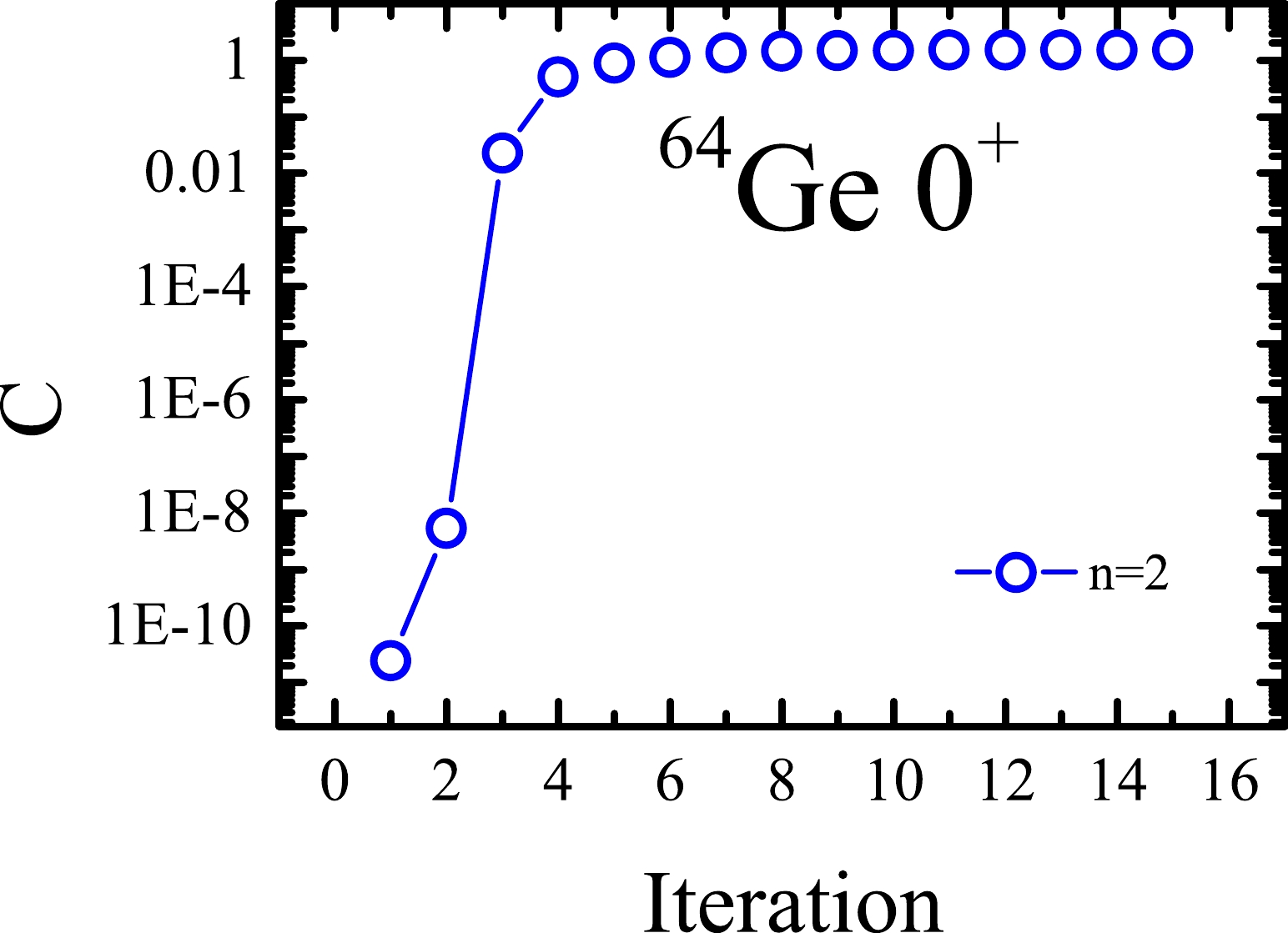
Figure 2. (color online) Iteration of the C quantity in Eq. (9) between the second candidate projected state and the
$ n=1 $ converged VAP wave function in Fig. 1 for the$ J^\pi=0^+ $ ground state in$ ^{64} $ Ge.With this useful projected SD
$ P^{J\pi}_{MK}|\Phi_2\rangle $ , one can perform the VAP calculation using Eq. (3). The calculation results are shown in Fig. 1. This time, the VAP energy is indeed reduced from$ -302.983 $ to$ -303.522 $ MeV. The corresponding coefficients in Eq. (3) become$f^{J\pi 1}_{1}= -3.3264+4.2404 {\rm i}$ and$f^{J\pi 1}_{2}=0.4038+6.6283 {\rm i}$ , which indicates that both projected states are important for the calculated state.With this new method, important projected SDs can be selected one by one so that the VAP iteration can be carried out normally. Thus, the VAP wave functions can be continuously improved. At this point, one can imagine that if the VAP process is omitted, the formed nuclear wave function is very similar to that in the MCSM [3]. However, the major difference is that, in the MCSM, the important projected SDs are selected from a large number of candidates, which are generated stochastically. Therefore, it seems that we have proposed an alternative method of basis selection, which can be used to replace that in the MCSM.
However, before we put more projected states into the VAP wave functions, we should solve another problem that is associated with the orthonormality among the included projected basis states, as will be addressed in the next section.
-
A natural deficiency of the projected states is their poor orthonormality among themselves. A direct consequence of this deficiency is the possible appearance of the redundant projected states, which seriously affects the stability of VAP iteration. This problem of orthonormality was addressed in Ref. [12]. In that work, the VAP calculation was performed so that the following Q quantity could be minimized:
$ \begin{equation} Q=\sum\limits_{\alpha=1}^{m} E_{\alpha}^{J\pi}+\chi_{1} \sum\limits_{i=1}^{n} \frac{1}{N_{i i}^{J\pi}}+\frac{\chi_{2}}{2} \sum\limits_{\substack{i, j=1 \\ i \neq j}}^{n} \frac{N_{i j}^{J\pi} N_{j i}^{J\pi}}{N_{i i}^{J\pi} N_{j j}^{J\pi}}, \end{equation} $

(10) where
$ N_{i j}^{J\pi}=\langle \Phi_i|P^{J\pi}_{KK}|\Phi_j\rangle $ . The first term is the sum of the calculated state energies, and the last two terms are constraints that are expected to keep the projected basis states in a good condition so that redundant states may not appear. One can easily understand that in Eq. (10), the second term tends to push the$ N_{i i}^{J\pi} $ norms to large values, and the third term tends to guide the projected basis states to be orthogonal to one another. Here, we propose a more reasonable constraint term that can be used to replace those two constraint terms in Eq. (10). The new definition of the Q quantity can be written as$ \begin{equation} Q=\sum\limits_{\alpha=1}^{m} E_{\alpha}^{J\pi}+\chi\frac{1}{|N^{J\pi}|}, \end{equation} $

(11) where
$ {|N^{J\pi}|} $ is the determinant of the norm matrix in Eq. (2). Notice that this$ |N^{J\pi}| $ value equals the product of all the eigenvalues of$ N^{J\pi} $ . If there is a redundant basis state, an eigenvalue of$ N^{J\pi} $ must be zero. Thus, the$ |N^{J\pi}| $ value also must be zero, and the constraint term in Eq. (11) becomes infinite, which is impossible. This means that the redundant state can be strictly forbidden by the new constraint term in Eq. (11). In contrast, the original constraints in Eq. (10) do not have such power in forbidding the appearance of redundant states. For instance, suppose that there are three normalized basis states$ |\phi_1\rangle $ ,$ |\phi_2\rangle $ , and$ |\phi_3\rangle $ , with the following relationships:$ \langle\phi_1|\phi_2\rangle=0 $ and$ |\phi_3\rangle=\frac{1}{\sqrt{2}}(|\phi_1\rangle+|\phi_2\rangle) $ . Then,$ |\phi_3\rangle $ is clearly a redundant state. In this case, one can easily obtain the value of the last term in Eq. (10), and it turns out to be$ \sqrt{2}\chi_2 $ , which seems not large enough to strongly restrict the basis states. Furthermore, this$ \frac{1}{|N^{J\pi}|} $ term tends to increase the eigenvalues of$ N^{J\pi} $ , playing a role similar to that of the second term in Eq. (10). Therefore, it is very nice to take the new constraint to keep the precision of the calculated VAP wave functions.In the present VAP calculations, the Q value in Eq. (11) needs to be minimized. Thus, it would be better for the gradient and the Hessian matrix of the
$ \frac{1}{|N^{J\pi}|} $ term to be calculated. Formulations of how to evaluate such quantities have been explicitly presented in the Appendix. Fortunately, all the required matrix elements for the$ \frac{1}{|N^{J\pi}|} $ term are actually available, because they were originally prepared for the gradient and the Hessian matrix of the VAP energies.To show the effect of this new
$ \frac{1}{|N^{J\pi}|} $ constraint, we perform the VAP calculations in the$ sd $ model space. Because this model space is quite small, the dimension of the corresponding configuration space is not so large that the randomly selected projected states can easily mix with one another. This makes it very convenient that one can avoid the complexity of combining this constraint with the first problem addressed in the previous section. Therefore, one can randomly generate a group of the projected SDs and directly perform the VAP calculation with or without the$ \frac{1}{|N^{J\pi}|} $ constraint.We randomly generate 10 projected SDs (
$ n=10 $ ) with$ K=0 $ to construct the lowest 5$ J^\pi=8^+ $ states ($ m=5 $ ) in$ ^{24} $ Mg. The USDB interaction [18] is adopted, and$ K=0 $ is taken. Then, the Q quantity in Eq. (11) is minimized with$ \chi=0 $ and$ \chi=0.01^{n} $ MeV$ =10^{-20} $ MeV, respectively. In principle, the χ parameter should be as small as possible provided that the VAP iteration can converge normally, so that the second term in Eq. (11) can be as small as possible. The associated quantities as functions of the VAP iteration are shown in Fig. 3. It is seen that without any constraint, the smallest eigenvalue of the$ N^{J\pi} $ shown in Fig. 3(a) tends to decrease, which is undesirable for obtaining precise VAP wave functions. Therefore, the gradient of Q in Fig. 3(b) is not accurately calculated, and it is very difficult for the gradient to be smaller than$ 10^{-3} $ MeV, which is the condition of our VAP convergence. Next, we perform the same calculation but with$ \chi=10^{-20} $ MeV. This time, the eigenvalues of$ N^{J\pi} $ do not become so small, and the VAP iteration converges quite fast. The VAP energies are compared with the exact shell model ones, and good approximation still can be achieved even with the new constraint. The final$\frac{\chi}{|N^{J\pi}|}$ value with$ \chi=10^{-20} $ MeV is found out to be$ 0.0056 $ MeV, which is sufficiently small.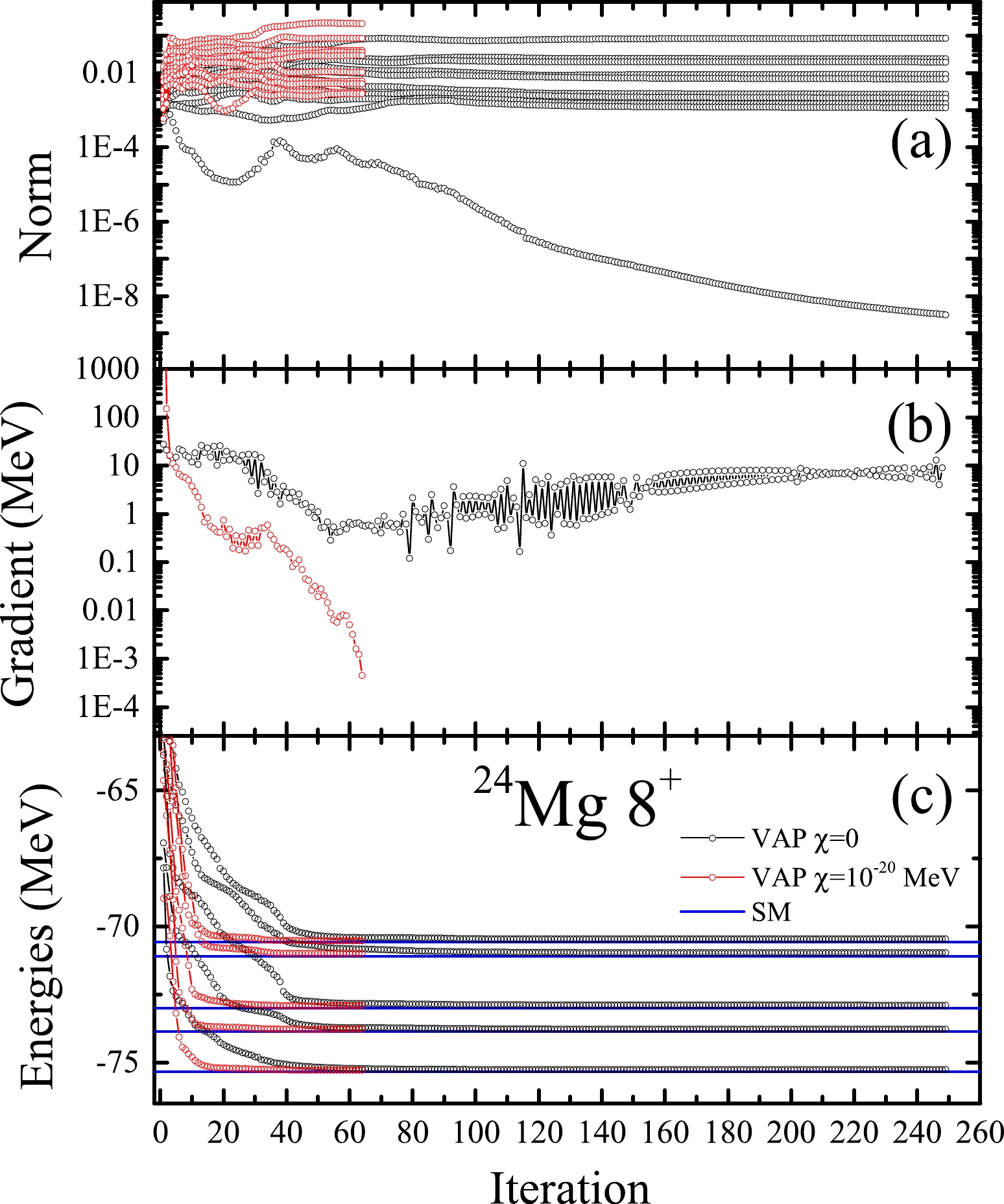
Figure 3. (color online) Calculated quantities as functions of the VAP iteration for the lowest five states (
$ m=5 $ ) with$ J^\pi=8^+ $ in$ ^{24} $ Mg. 10 projected SDs are adopted to construct the VAP wave functions. The USDB interaction is adopted. (a) Calculated 10 eigenvalues of$ N^{J\pi} $ ; (b) absolute value of the gradient of the Q quantity; (c) calculated lowest five energies. The shell model (SM) energies are also shown, for comparison. -
The above two problems may appear simultaneously in a VAP calculation. Suppose that there are m lowest states that need to be calculated. The VAP calculation can be performed in two steps. In the first step, one generates
$ n=m $ projected SDs randomly and constructs the simplest VAP wave functions for these m lowest states. Then, these wave functions are varied simultaneously so that the Q quantity with$ \chi\neq 0 $ in Eq. (11) can be minimized. The second step is to improve the VAP wave functions by adding a useful projected state using the algorithm addressed in Sec. II. Then, one can perform the same VAP iteration as in the first step but with$ n=m+1 $ . In this way, projected SDs can be effectively added one by one, and the approximations of the calculated m lowest states can be continuously improved.As a practical example, we calculate the lowest
$ J^\pi=4^+ $ states in$ ^{56} $ Ni. The GXPF1A interaction [17] in the$ pf $ shell model space is adopted, and$ K=0 $ is taken. The constraint parameter χ is assumed to be associated with the number of included projected states and is simply taken to be$ \chi=10^{-2n} $ MeV. We first calculate the yrast state ($ m=1 $ ). The results are shown in Fig. 4. It is shown that the calculated energy decreases steadily with the addition of projected SDs one by one. This clearly indicates that each of the added projected states is indeed important for the lowest$ J^\pi=4^+ $ state. One can also see that the energy decreases rapidly at the beginning, and the decrease slows as n increases. This can be understood as follows: at each n, the most important projected state should be obtained because it reduces the energy to the maximum value in the VAP algorithm. This means that the next added projected state should be less important than the previous one.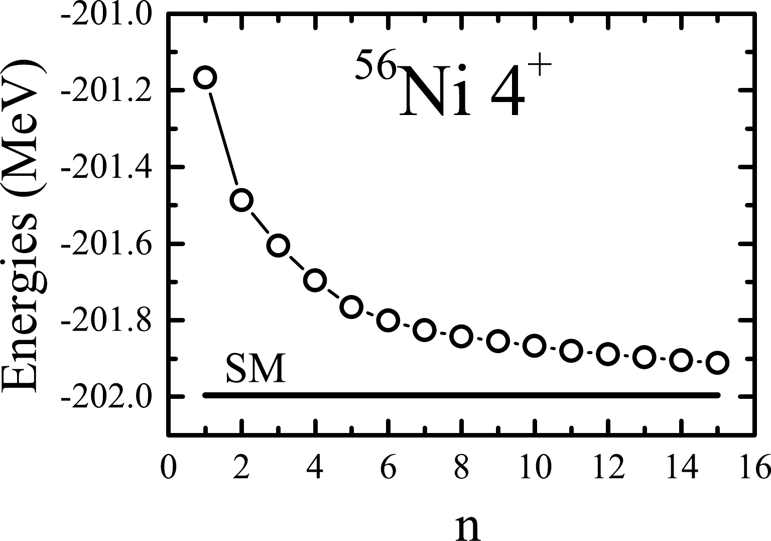
Figure 4. Lowest (yrast) energy of
$ J^\pi=4^+ $ in$ ^{56} $ Ni calculated with the present VAP as a function of n, i.e., the number of included projected basis states. The shell model (SM) energy is shown for comparison.Next, we calculate the lowest three
$ 4^+ $ states in$ ^{56} $ Ni, simultaneously. The calculation results are shown in Fig. 5. It is seen that all the calculated energies decrease as n increases, which seems very similar to the trend in Fig. 4. However, one can also see in Fig. 5 that the energies are not always significantly improved by adding a new projected state. As mentioned previously, if the added new projected state does not mix with one of the state wave functions, the corresponding energy remains unchanged. From Fig. 5, one can understand that the selected new projected state can be important for at least one of the calculated states but may not always be important for all of them. Nevertheless, it is believed that the calculated three energies may be sufficiently close to the exact shell model ones if n is large enough. Unfortunately, this requires more computational time, and one should consider how to perform the VAP calculation more efficiently. This is another important issue that should be seriously studied in the future.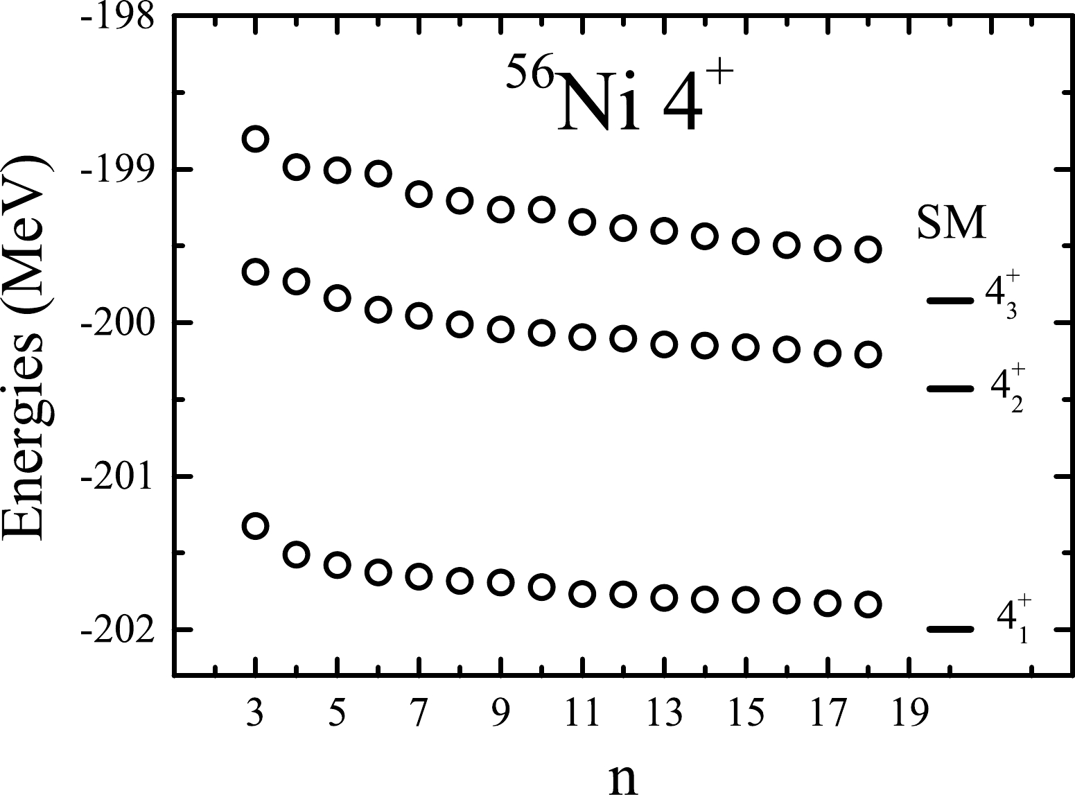
Figure 5. Similar to Fig. 4 but for the lowest three energies of
$ J^\pi=4^+ $ in$ ^{56} $ Ni. -
The projected wave functions with good quantum numbers are effective blocks for the construction of nuclear wave functions. The full optimized nuclear wave functions expanded in terms of these projected states can be obtained through the VAP calculation. However, when the VAP calculations are performed in a large model space, very few randomly selected projected basis states are scattered in an extremely huge configuration space. This means that the selected projected basis states are likely to be too different to be linked by the Hamiltonian. In other words, Eq. (4) always holds when
$ |\psi\rangle $ and$ |\phi\rangle $ refer to different projected basis states in a huge configuration space. Thus, in a large model space, the randomly selected projected state is likely to be irrelevant for the calculated states. To solve this problem, we propose an algorithm whereby such irrelevant projected states can be varied so that they can be important for the calculated states. However, we never encounter such a problem in the small$ sd $ model space, because the configuration space is very small. Another problem is that the projected basis states are far from orthonormality, which seriously reduces the stability of the VAP iteration. We solve this problem by imposing a new constraint on the sum of the calculated energies. The proposed solutions for the discussed problems are supported by the calculated examples.Certainly, the discussed problems are general ones and are independent of the specific form of the basis states. Thus, the present work may be helpful in developing various quantum many-body methods. For instance, if the VAP wave functions are formed with the projected Hartree-Fock-Bogoliubov quasipaticle vacuum states, one may still encounter the same two problems. In this case, we expect that the present solutions would still be valid, which will be further investigated in the future. For another example, in the GCM method, one can generate numerous basis states by varying different deformation parameters. Then, one does not need to include all the GCM basis states but just pick up some of the most important ones one by one by evaluating the C quantity for each basis state. Other possible applications will be investigated in the future.
-
For simplicity, let us rewrite the constraint term as follows:
$ Q_0=\frac{1}{\left|\begin{array}{lll} N_{11} &\cdots& N_{1n}\\ &\cdots& \\ N_{n1} &\cdots& N_{nn} \end{array}\right|}=\frac{1}{|N| }, \tag{A1} $

where
$ N_{i j}=\langle \Phi_i|P^{J\pi}_{KK}|\Phi_j\rangle $ . In the VAP method, one can vary the$ |\Phi_i\rangle $ states by applying the Thouless theorem to find the best set of VAP basis states [19]:$ |\Phi_i\rangle=\mathcal{N} {\rm e}^{\frac{1}{2} \sum _{\mu \nu} d_{\mu \nu} \beta_{0,\mu }^{\dagger}\beta_{0,\nu }^{\dagger}}|\Phi_{0}\rangle=\mathcal{N} {\rm e}^{ \sum _{\mu<\nu} d_{\mu \nu} A_{\mu \nu }^{\dagger}}|\Phi_{0}\rangle, \tag{A2} $

where
$ \mathcal{N} $ is the normalization parameter.$ A_{\mu \nu }^{\dagger} $ is generally a quasiparticle pair operator corresponding to the fixed$ |\Phi_{0}\rangle $ HFB vacuum state, but here it refers to a particle-hole operator, and$ |\Phi_{0}\rangle $ is a Slater determinant. d is a complex skew matrix. The matrix elements$ d_{\mu \nu} $ can be complex numbers:$ d_{\mu \nu}=x_{\mu \nu}+{\rm i} y_{\mu \nu}. \tag{A3} $

where
$ x_{\mu \nu} $ and$ y_{\mu \nu} $ are real numbers and are the variational parameters. For convenience, we use$ x_\alpha $ ,$ x_\beta $ , etc., to represent these variational parameters.Then, the gradient of
$ Q_0 $ can be expressed as$ \begin{aligned}[b] \frac{\partial Q_0}{\partial x_{\alpha}}=-\frac{1}{|N |^2}\frac{\partial |N | }{\partial x_{\alpha}}=-\frac{1}{|N |^2}\sum\limits_{i=1}^n\left|\begin{array}{lll} N_{11} &\cdots& N_{1n} \\ &\cdots& \\ \frac{\partial N_{i1} }{\partial x_{\alpha}} &\cdots& \frac{\partial N_{in} }{\partial x_{\alpha}} \\ &\cdots& \\ N_{n1} &\cdots& N_{nn} \end{array}\right| \end{aligned} $

$ \begin{aligned}[b] =-\frac{1}{|N |^2}\sum\limits_{i,k=1}^n\frac{\partial N_{i k} }{\partial x_{\alpha}}\overline{N }\{i|k\} , \end{aligned}\tag{A4} $

where
$ \overline{N }\{i|k\}=(-1)^{i+k}|N \{i|k\}| $ is a cofactor of$ |N | $ . The submatrix$ N \{i|k\} $ is obtained by removing the ith row and kth column from the matrix N. If the variational parameter$ x_\alpha $ is the real part of$ d_{\mu \nu} $ ,$ \dfrac{\partial N_{i k} }{\partial x_{\alpha}}=\dfrac{\partial N_{i k} }{\partial x_{\mu \nu}} $ can be expressed as follows:$ \frac{\partial N_{ik} }{\partial x^k_{\mu \nu}}= \langle\Phi_{i}| P_{KK}^{J\pi} A_{\mu\nu}^{k\dagger}| \Phi_{k}\rangle, \tag{A5} $

$ \frac{\partial N_{ik} }{\partial x^i_{\mu \nu}}=\langle\Phi_{i}| A^i_{\mu\nu} P_{KK}^{J\pi}| \Phi_{k}\rangle, \tag{A6} $

$ \frac{\partial N_{ii} }{\partial x^i_{\mu \nu}}=\langle\Phi_i|P_{K K}^{J\pi} A_{\mu\nu}^{i\dagger}| \Phi_i\rangle+\langle\Phi_i|A^i_{\mu\nu} P_{K K}^{J\pi}| \Phi_i\rangle. \tag{A7} $

If the variational parameter
$ x_\alpha $ is the imaginary part of$ d_{\mu \nu} $ ,$ \dfrac{\partial N_{i k} }{\partial x_{\alpha}}=\dfrac{\partial N_{i k} }{\partial y_{\mu \nu}} $ can be expressed as follows:$ \frac{\partial N_{ik} }{\partial y^k_{\mu \nu}}={\rm i}\langle\Phi_{i}| P_{KK }^{J\pi} A_{\mu \nu}^{k\dagger}| \Phi_{k}\rangle, \tag{A8}$

$ \frac{\partial N_{ik} }{\partial y^i_{\mu \nu}}=-{\rm i}\langle\Phi_{i}| A^i_{\mu \nu} P_{KK}^{J\pi}| \Phi_{k}\rangle, \tag{A9} $

$ \frac{\partial N_{ii} }{\partial y^i_{\mu \nu}}={\rm i}\langle\Phi_i|P_{K K}^{J\pi} A_{\mu \nu}^{i\dagger}| \Phi_i\rangle-{\rm i}\langle\Phi_i|A_{\mu \nu}^i P_{K K}^{J\pi}| \Phi_i\rangle. \tag{A10} $

Details can be found in Ref. [10].
Similarly, the Hessian of
$ Q_0 $ can be written as$ \frac{\partial^2 Q_0}{\partial x_{\alpha}\partial x_{\beta} }=2\frac{1}{|N |^3}\frac{\partial |N | }{\partial x_{\alpha}}\frac{\partial |N |}{\partial x_{\beta}}-\frac{1}{|N |^2}\frac{\partial^2 |N | }{\partial x_{\alpha}\partial x_{\beta}}, \tag{A11} $

where the
$ \dfrac{\partial^2 |N | }{\partial x_{\alpha}\partial x_{\beta}} $ in the second term of Eq. (A11) can be calculated using the following equation:$ \dfrac{\partial^2 |N | }{\partial x_{\alpha}\partial x_{\beta}} =\sum\limits_{i=1}^n\left|\begin{array}{lll} N_{11} &\cdots& N_{1n} \\ &\cdots& \\ \dfrac{\partial^2 N_{i1} }{\partial x_{\alpha}\partial x_{\beta}} &\cdots& \dfrac{\partial ^2N_{in} }{\partial x_{\alpha}\partial x_{\beta}} \\ &\cdots& \\ N_{n1} &\cdots& N_{nn} \end{array}\right| $

$ \begin{aligned}[b] &+\sum\limits_{i,j=1\atop i\neq j}^n\left|\begin{array}{lll} N_{11} &\cdots& N_{1n} \\ &\cdots& \\ \dfrac{\partial N_{i1} }{\partial x_{\alpha} } &\cdots& \dfrac{\partial N_{in} }{\partial x_{\alpha} } \\ &\cdots& \\ \dfrac{\partial N_{j1} }{ \partial x_{\beta}} &\cdots& \dfrac{\partial N_{in} }{ \partial x_{\beta}} \\ &\cdots& \\ N_{n1} &\cdots& N_{nn} \end{array}\right| \\ =&\sum\limits_{i,k=1}^n\frac{\partial^2 N_{i k} }{\partial x_{\alpha}\partial x_{\beta}}\overline{N }\{i|k\} \\ &+ \sum\limits_{ijkl,\atop i\neq j, (k<l)}\left|\begin{array}{ll} \dfrac{\partial N_{ik} }{\partial x_{\alpha}} & \dfrac{\partial N_{il} }{\partial x_{\alpha}}\\ \dfrac{\partial N_{jk} }{\partial x_{\beta}} & \dfrac{\partial N_{jl} }{\partial x_{\beta}} \end{array}\right|\overline{N }\{ij|kl\}. \\ \end{aligned}\tag{A12} $

If
$ i < j $ and$ k < l $ , then$ \overline{N }\{ij|kl\} $ is usually called the second order cofactor and is defined as$ \overline{N }\{ij|kl\}=(-1)^{i+j+k+l}|N \{ij|kl\}|, \tag{A13}$

where the submatrix
$ N \{ij|kl\} $ is obtained from the matrix N by removing the$ i,j $ th rows and$ k,l $ th columns.Both
$ \overline{N }\{i|k\} $ and$ \overline{N }\{ij|kl\} $ can be easily obtained by using Jacobi's identity in the matrix theory [20]:$ \overline{N }\{i|k\}={N_{ki} }^{-1}|N |, \tag{A14} $

$ \begin{array}{*{20}{l}} \overline{N }\{ij|kl\}= \left|\begin{array}{ll} {N_{ki} }^{-1} & {N_{kj} }^{-1}\\ {N_{li} }^{-1} & {N_{lj} }^{-1} \end{array}\right||N |. \end{array} \tag{A15}$

The expression of
$ \dfrac{\partial^2 N_{i k} }{\partial x_{\alpha}\partial x_{\beta}} $ can be obtained as follows. If the variational parameters$ x_{\alpha} $ and$ x_{\beta} $ are the real parts of$ d_{\mu \nu} $ , then$ \dfrac{\partial^2 N_{i k} }{\partial x_{\alpha}\partial x_{\beta}}= \dfrac{\partial^2 N_{i k} }{\partial x_{\mu \nu}\partial x_{\mu' \nu'}} $ , and we have$ \frac{\partial^2 N_{ik}}{\partial x^k_{\mu \nu}\partial x^k_{\mu' \nu'}} = \langle\Phi_i | P_{KK }^{J\pi}A_{\mu \nu}^{k\dagger}A_{\mu' \nu'}^{k\dagger}|\Phi_{k}\rangle-N_{ik}\delta_{\mu\mu'\nu\nu'},\tag{A16} $

$ \frac{\partial^2 N_{ik}}{\partial x^i_{\mu \nu}\partial x^i_{\mu' \nu'}} = \langle\Phi_{i}|A^i_{\mu' \nu'}A^i_{\mu \nu} P_{KK }^{J\pi} |\Phi_{k}\rangle-N_{ik}\delta_{\mu\mu' \nu\nu'},\tag{A17} $

$ \frac{\partial^2 N_{ik}}{\partial x^i_{\mu \nu}\partial x^k_{\mu' \nu'}} = \langle\Phi_{i}|A^i_{\mu \nu} P_{KK }^{J\pi}A_{\mu' \nu'}^{k\dagger}|\Phi_{k}\rangle, \tag{A18}$

$ \begin{aligned}[b] \frac{\partial^2 N_{ii}}{\partial x^i_{\mu \nu}\partial x^i_{\mu' \nu'}} =&\langle\Phi_{i}|A^i_{\mu' \nu'}A^i_{\mu \nu} P_{KK }^{J\pi}|\Phi_{i }\rangle\\ & +\langle\Phi_{i}|A^i_{\mu \nu} P_{KK }^{J\pi}A_{\mu' \nu'}^{i\dagger}|\Phi_{i }\rangle\\ & +\langle\Phi_{i}|A^i_{\mu' \nu'} P_{KK }^{J\pi}A_{\mu \nu}^{i\dagger}|\Phi_{i }\rangle\\ & + \langle\Phi_i | P_{KK }^{J\pi}A_{\mu \nu}^{i\dagger}A_{\mu' \nu'}^{i\dagger}|\Phi_{i}\rangle- 2N_{ii}\delta_{\mu\mu' \nu\nu'}. \end{aligned} \tag{A19}$

If the variational parameter
$ x_{\alpha} $ is the real part and$ x_{\beta} $ is the imaginary part of$ d_{\mu \nu} $ , then$ \dfrac{\partial^2 N_{i k} }{\partial x_{\alpha}\partial x_{\beta}}= \dfrac{\partial^2 N_{i k} }{\partial x_{\mu \nu}\partial y_{\mu' \nu'}} $ , and we have$ \frac{\partial^2 N_{ik}}{\partial x^k_{\mu \nu}\partial y^k_{\mu' \nu'}} = {\rm i}\langle\Phi_i | P_{KK }^{J\pi}A_{\mu \nu}^{k\dagger}A_{\mu' \nu'}^{k\dagger}|\Phi_{k}\rangle,\tag{A20} $

$ \frac{\partial^2 N_{ik}}{\partial x^i_{\mu \nu}\partial y^i_{\mu' \nu'}}=-{\rm i} \langle\Phi_{i}|A^i_{\mu' \nu'}A^i_{\mu \nu} P_{KK }^{J\pi} |\Phi_{k}\rangle, \tag{A21} $

$ \frac{\partial^2 N_{ik}}{\partial x^i_{\mu \nu}\partial y^k_{\mu' \nu'}} = {\rm i} \langle\Phi_{i}|A^i_{\mu \nu} P_{KK }^{J\pi}A_{\mu' \nu'}^{k\dagger}|\Phi_{k}\rangle, \tag{A22} $

$ \begin{aligned}[b] \frac{\partial^2 N_{ii}}{\partial x^i_{\mu \nu}\partial y^i_{\mu' \nu'}} =&-{\rm i}\langle\Phi_{i}|A^i_{\mu' \nu'}A^i_{\mu \nu} P_{KK }^{J\pi}|\Phi_{i }\rangle\\ & +{\rm i}\langle\Phi_{i}|A^i_{\mu \nu} P_{KK }^{J\pi}A_{\mu' \nu'}^{i\dagger}|\Phi_{i }\rangle\\ & -{\rm i}\langle\Phi_{i}|A^i_{\mu' \nu'} P_{KK }^{J\pi}A_{\mu \nu}^{i\dagger}|\Phi_{i }\rangle\\ & +{\rm i} \langle\Phi_i | P_{KK }^{J\pi}A_{\mu \nu}^{i\dagger}A_{\mu' \nu'}^{i\dagger}|\Phi_{i}\rangle. \end{aligned} \tag{A23}$

If the variational parameter
$ x_{\alpha} $ is the imaginary part and$ x_{\beta} $ is the real part of$ d_{\mu \nu} $ , then$ \dfrac{\partial^2 N_{i k} }{\partial x_{\alpha}\partial x_{\beta}}= \dfrac{\partial^2 N_{i k} }{\partial y_{\mu \nu}\partial x_{\mu' \nu'}} $ , and we have$ \frac{\partial^2 N_{ik}}{\partial y^k_{\mu \nu}\partial x^k_{\mu' \nu'}} = {\rm i}\langle\Phi_i | P_{KK }^{J\pi}A_{\mu \nu}^{k\dagger}A_{\mu' \nu'}^{k\dagger}|\Phi_{k}\rangle, \tag{A24} $

$ \frac{\partial^2 N_{ik}}{\partial y^i_{\mu \nu}\partial x^i_{\mu' \nu'}} = -{\rm i}\langle\Phi_{i}|A^i_{\mu' \nu'}A^i_{\mu \nu} P_{KK }^{J\pi} |\Phi_{k}\rangle, \tag{A25} $

$ \frac{\partial^2 N_{ik}}{\partial y^i_{\mu \nu}\partial x^k_{\mu' \nu'}} = -{\rm i} \langle\Phi_{i}|A^i_{\mu \nu} P_{KK }^{J\pi}A_{\mu' \nu'}^{k\dagger}|\Phi_{k}\rangle, \tag{A26} $

$ \begin{aligned}[b] \frac{\partial^2 N_{ii}}{\partial y^i_{\mu \nu}\partial x^i_{\mu' \nu'}} =-{\rm i}\langle\Phi_{i}|A^i_{\mu' \nu'}A^i_{\mu \nu} P_{KK }^{J\pi}|\Phi_{i }\rangle \end{aligned} $

$ \begin{aligned}[b] &-{\rm i}\langle\Phi_{i}|A^i_{\mu \nu} P_{KK }^{J\pi}A_{\mu' \nu'}^{i\dagger}|\Phi_{i }\rangle +{\rm i}\langle\Phi_{i}|A^i_{\mu' \nu'} P_{KK }^{J\pi}A_{\mu \nu}^{i\dagger}|\Phi_{i }\rangle\\ & +{\rm i} \langle\Phi_i | P_{KK }^{J\pi}A_{\mu \nu}^{i\dagger}A_{\mu' \nu'}^{i\dagger}|\Phi_{i}\rangle. \end{aligned}\tag{A27} $

If the variational parameters
$ x_{\alpha} $ and$ x_{\beta} $ are the imaginary parts of$ d_{\mu \nu} $ , then$ \dfrac{\partial^2 N_{i k} }{\partial x_{\alpha}\partial x_{\beta}}= \dfrac{\partial^2 N_{i k} }{\partial y_{\mu \nu}\partial y_{\mu' \nu'}} $ , and we have$ \frac{\partial^2 N_{ik}}{\partial y^k_{\mu \nu}\partial y^k_{\mu' \nu'}} = -\langle\Phi_i | P_{KK }^{J\pi}A_{\mu \nu}^{k\dagger}A_{\mu' \nu'}^{k\dagger}|\Phi_{k}\rangle-N_{ik}\delta_{\mu\mu'\nu\nu'}, \tag{A28} $

$ \frac{\partial^2 N_{ik}}{\partial y^i_{\mu \nu}\partial y^i_{\mu' \nu'}} = -\langle\Phi_{i}|A^i_{\mu' \nu'}A^i_{\mu \nu} P_{KK }^{J\pi} |\Phi_{k}\rangle-N_{ik}\delta_{\mu\mu'\nu\nu'}, \tag{A29}$

$ \frac{\partial^2 N_{ik}}{\partial y^i_{\mu \nu}\partial y^k_{\mu' \nu'}} = \langle\Phi_{i}|A^i_{\mu \nu} P_{KK }^{J\pi}A_{\mu' \nu'}^{k\dagger}|\Phi_{k}\rangle, \tag{A30} $

$ \begin{aligned}[b] \frac{\partial^2 N_{ii}}{\partial y^i_{\mu \nu}\partial y^i_{\mu' \nu'}}=&-\langle\Phi_{i}|A^i_{\mu' \nu'}A^i_{\mu \nu} P_{KK }^{J\pi}|\Phi_{i }\rangle\\ & +\langle\Phi_{i}|A^i_{\mu \nu} P_{KK }^{J\pi}A_{\mu' \nu'}^{i\dagger}|\Phi_{i }\rangle\\ & +\langle\Phi_{i}|A^i_{\mu' \nu'} P_{KK }^{J\pi}A_{\mu \nu}^{i\dagger}|\Phi_{i }\rangle\\ & - \langle\Phi_i | P_{KK }^{J\pi}A_{\mu \nu}^{i\dagger}A_{\mu' \nu'}^{i\dagger}|\Phi_{i}\rangle- 2N_{ii}\delta_{\mu\mu'\nu\nu'}. \end{aligned}\tag{A31} $

Finding optimal basis states for variation after projection nuclear wave functions
- Received Date: 2023-02-28
- Available Online: 2023-07-15
Abstract: The variation after projection (VAP) method is expected to be an efficient way of obtaining the optimized nuclear wave functions, which can be as close as possible to the exact shell model ones. However, we found that there are two additional problems that may seriously affect the convergence of the VAP iteration. The first problem is the existence of irrelevant projected basis states. At a VAP iteration, the Hill-Wheeler (HW) equation is composed of all updated projected basis states. If one of these projected basis states does not mix with a calculated wave function of interest, which is obtained by solving this HW equation, it is likely that this basis state will never mix with this wave function even after the VAP iteration converges. The other problem is the poor orthonormality among the projected basis states, which seriously affects the accuracy of the calculated VAP wave function. In the present work, solutions for these two problems are proposed, and examples are presented to test the validity. With the present solutions, the most important projected basis states can be reliably obtained, and the fully optimized VAP wave functions can be accurately and efficiently calculated.


 DownLoad: