Triangle mechanism in the decay process $ {\boldsymbol B_{\bf 0}{\bf \to}{\boldsymbol J}{\bf /}\boldsymbol\psi {\boldsymbol K}^{\bf 0} {\boldsymbol f}_{\bf 0}{\bf (980)}({\boldsymbol a}_{\bf 0}{\bf(980))} }$

The dynamics of the strong interaction are described by quantum chromodynamics (QCD), and hadron spectroscopy is a method of studying QCD; meanwhile, hadron spectroscopy is the basic theory of the strong interaction. Understanding the spectrum of hadron resonances [1] and establishing a connection with the QCD is one of the important goals of hadron physics. The conventional quark models in the low-lying hadron spectrum successfully explain that a baryon is a complex of three quarks, and a meson is a combination of a quark and an antiquark [2, 3]. However, even if the model provides a large amount of data about the meson and baryon resonances [2–4], we cannot rule out other more exotic components, especially considering that the QCD Lagrangian includes not only quarks but also gluons. This leads to other configurations of color singlets, such as glueballs made purely of gluons, mixed states made of quark and gluon excitations, and multiquarks. There is also the possibility of more quark states in a hadron, such as $ qq\bar{q}\bar{q} $ and $ qq\bar{q}qq $, which are mentioned in Ref. [5]. To quantitatively understand the QCD of quarks and gluons, over the years, numerous related experiments have been conducted in search of evidence for these exotic components in the mesonic and baryonic spectrum [6–10].

The triangle singularity (TS) was discussed in Ref. [11], and Landau has systematized it in Ref. [12]. The TS was fashionable in the 1960s [13–16]. In addition to ordinary hadronic, molecular, or multiquarks states, TSs can produce peaks, but these peaks are produced by kinematic effects. The Coleman-Norton theorem [17] states that the Feynman amplitude has a singularity on the physical boundary as time moves forward if the decay process can be interpreted as taking place during the conservation of energy and momentum in space-time, and all internal particles really exist on the shell. In the process of particle 1 decaying into particles 2 and 3, particle 1 first decays into particles A and B, then A decays into particles 2 and C, and finally particles B and C fuse into an external particle 3. Particles A, B, and C are intermediate particles, and if the momenta of these intermediate particles can take on-shell values, a singularity will occur. A simpler and more practical way to understand this process was proposed in Ref. [18]; this method does not compute the entire amplitude of the Feynman diagram including the triangle loop. The condition for producing a TS is $q_{\rm on+}=q_{a-}$, as given by Eq. (18) in Ref. [18], where $q_{\rm on}$ represents the on-shell momentum of particle A or B in the rest system of particle 1, and $ q_{a-} $ defines one of the two solutions to the momentum of particle B when B and C produce particle 3 on the shell. Since the process of the triangle mechanism involves the fusion of hadrons, the presence of hadronic molecular states plays an important role in having measurable strength. Therefore, the study of singularity is also a useful tool to study the molecular states of hadrons.

The isospin violation in production of the $ f_0(980) $ or $ a_0(980) $ resonance generation and its mixing have long been controversial. We have to give up the idea of trying to establish a "$ f_0-a_0 $ mixing parameter" from different reactions, because it was shown that the isospin violation depends significantly on the reaction [19–22]. The spark was raised by the puzzle of the anomalously large isospin violation in the $ \eta(1450)\to\pi^0f_0(980) $ decay [23], which was due to a TS and was explained in Refs. [21, 22]. From the point of view of the $ f_0(980) $ and $ a_0(980) $ themselves, the above reaction is very enlightening. These resonances are produced by the rescattering of $ K\bar{K} $, i.e., the mechanism for the formation of these resonances in the chiral unitary approach [24–27]. In addition, there are numerous processes with the same mechanism, such as the process $ \tau^-\to\nu_{\tau}\pi^-f_0 (a_0) $ [28], the process $B^0_s\to J/\psi\pi^0f_0(a_0)$ [29], the process $ D_s^+\to\pi^+\pi^0f_0(a_0) $ [30], and the process $ B^-\to D^{\ast 0}\pi^-f_0(a_0) $ [31], and the same TS was shown in Refs. [32, 33] to provide a plausible explanation for the peak observed in the $ \pi f_0(980) $ final state. It is easy to envisage many reactions of this type [34], and this inspires us to find more processes like this type and search for TS enhanced isospin-violating reactions producing the $ f_0(980) $ or $ a_0(980) $ resonances [35].

In the present study, we investigate the reactions $ B^0\to J/\psi K^0f_0(980) $ and $ B^0\to J/\psi K^0a_0(980) $; both decay modes are allowed. The process followed by the ϕ decay into $ K^0\bar{K}^0 $ and $ K^0\bar{K}^0 $ fuse into $ f_0(a_0) $ to generate a singularity, and the TS in this process contains relevant information concerning the nature of the $ f_0(980) $ and $ a_0(980) $ resonances. We show that it develops a TS at an invariant mass $ M_{\rm inv}(K^0R)\simeq1520\ {\rm MeV} $. Meanwhile, we can obtain ${{\rm d}^2\Gamma}/{[{\rm d} M_{\rm inv}(K^0f_0){\rm d} M_{\rm inv}(\pi^+\pi^-)]}$ or ${{\rm d}^2\Gamma}/ {[{\rm d}M_{\rm inv}(K^0a_0){\rm d}M_{\rm inv}(\pi^0\eta)]}$, which show the shapes of the $ f_0 $(980) and $ a_0 $(980) resonances in the $ \pi^+\pi^- $ or $ \pi^0\eta $ mass distributions, respectively. We can restrict the integral in $ M_{\rm inv}(\pi^+\pi^-) $ or $ M_{\rm inv}(\pi^0\eta) $ to this region when calculating the mass distribution ${{\rm d}^2\Gamma}/{[{\rm d}M_{\rm inv}(K^0f_0){\rm d}M_{\rm inv}(\pi^+\pi^-)]}$ or ${{\rm d}^2\Gamma}/{[{\rm d}M_{\rm inv}(K^0a_0){\rm d}M_{\rm inv}(\pi^0\eta)]}$. Then, we integrate over the $ \pi^+\pi^- $ or $ \pi^0\eta $ invariant masses and obtain a clear peak around $ M_{\rm inv}(K^0R)\simeq1520\ {\rm MeV} $. The further integration over $ M_{\rm inv}(K^0R) $ provides us branching ratios for $ B^0\to J/\psi K^0\pi^+\pi^- B^0\to J/\psi K^0\pi^0\eta $, and we find that the mass distribution of these decay processes shows a peak associated with TS. In addition, the corresponding decay branching ratio is obtained, and we obtain the branching fractions $ {\rm Br}(B_0\to J/\psi K^0f_0(a_0))=1.007\times10^{-5} $, ${\rm Br}(B_0 \to J/\psi K^0f_0(980)\to J/\psi K^0\pi^+\pi^-)=1.38\times10^{-6}$, and ${\rm Br}(B_0\to J/\psi K^0a_0(980)\to J/\psi K^0\pi^0\eta)=2.56\times10^{-7}$. In any case, the main aim of the present work is to point out the presence of the TS in this reaction. This work provides one more measurable example of a TS, which has been quite sparse up to now. The singularity generated by this process can also play an early warning role for future experiments.

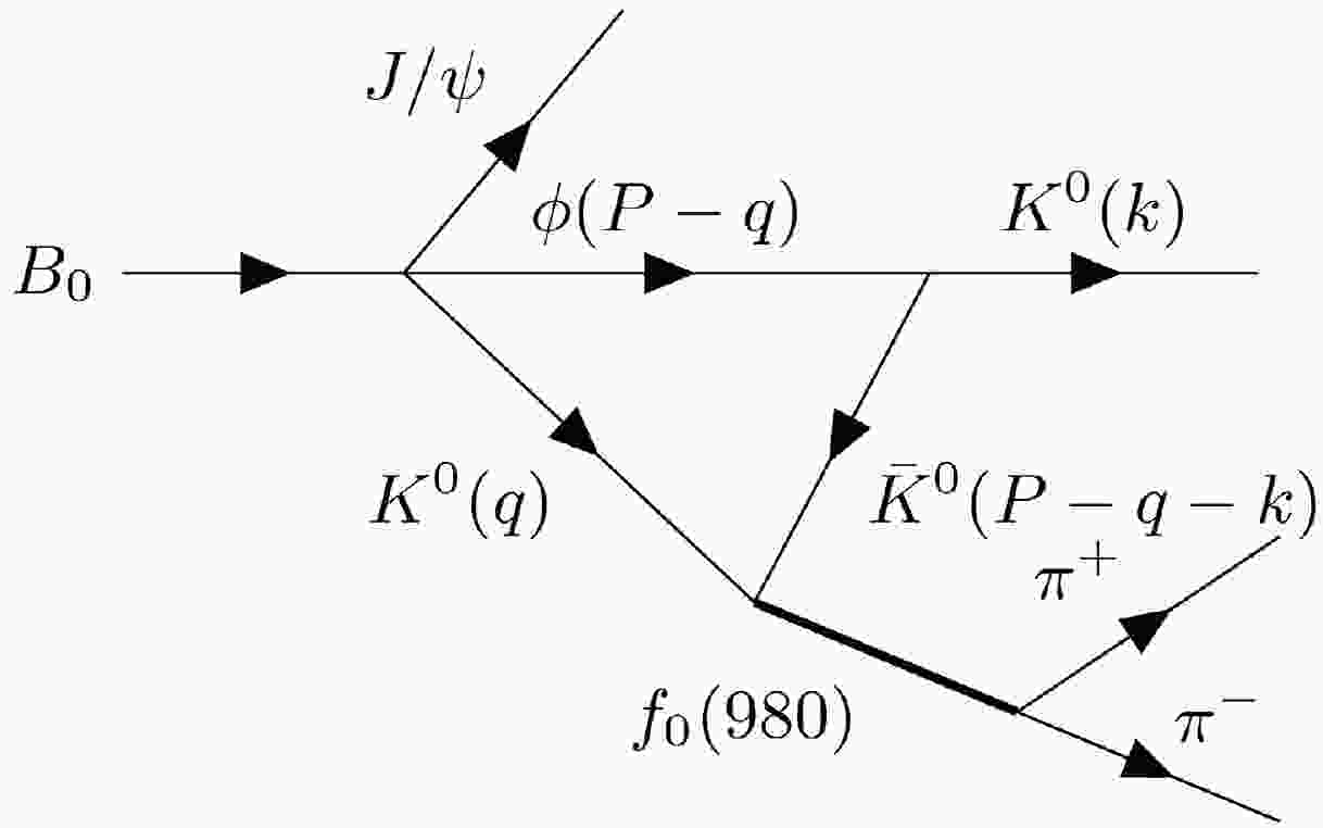
We plot the Feynman digrams of the decay process $ B_0 \to J/\psi K^0 f_0(a_0)(980) $ involving a triangle loop in Figs. 1 and 2. We observe that particle $ B_0 $ first decays into particles $ J/\psi, \phi, K^0 $, and then, particle ϕ decays into$ K^0 $ and $ \bar{K}^0 $; then, $ K^0 $ and $ \bar{K}^0 $ fuse into $ f_0(a_0) $, and eventually $ f_0(a_0) $ decays into $ \pi^+\pi^-(\pi^0\eta) $.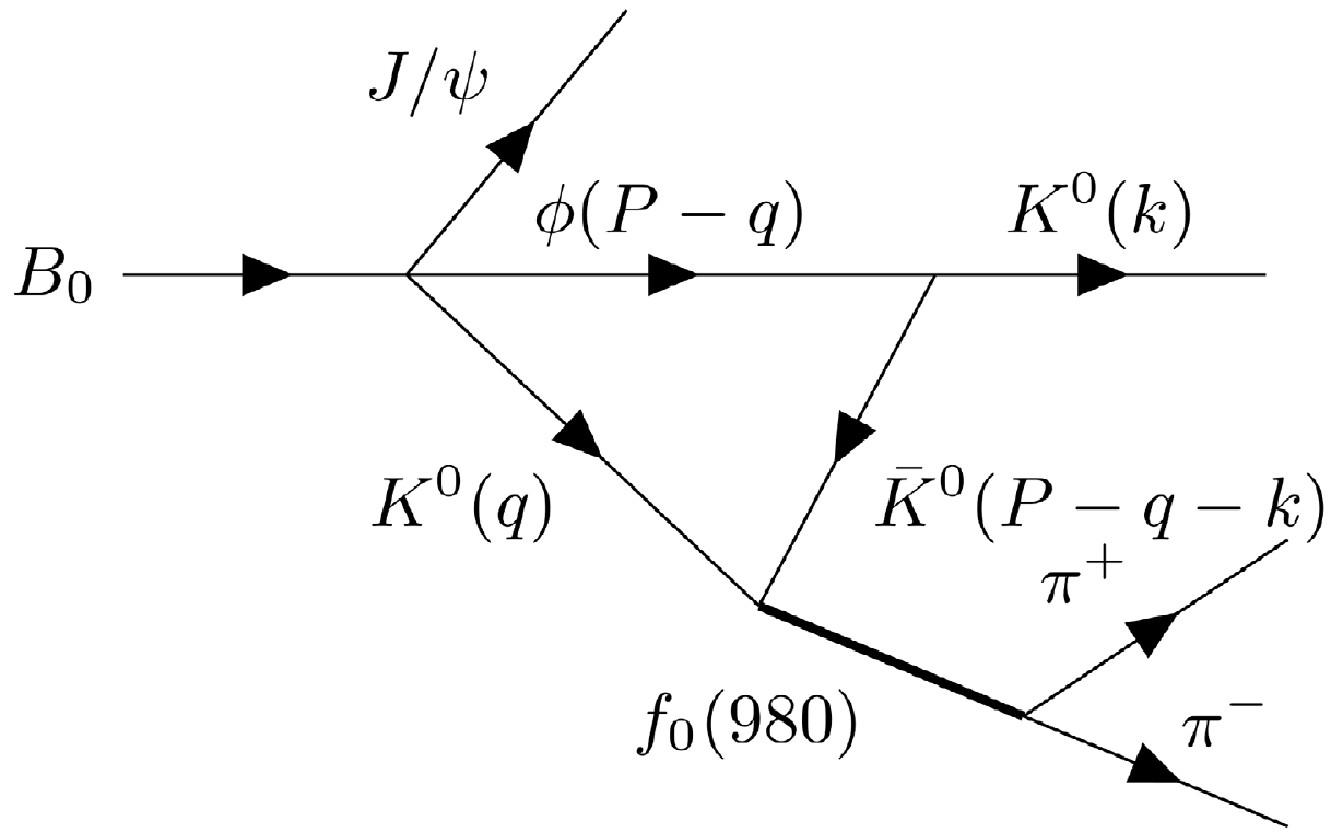

Figure 1.  Feynman diagrams of the decay process $B_0 \to $$ J/\psi K^0 f_0(980)\to J/\psi K^0\pi^+ \pi^-$ involving a triangle loop.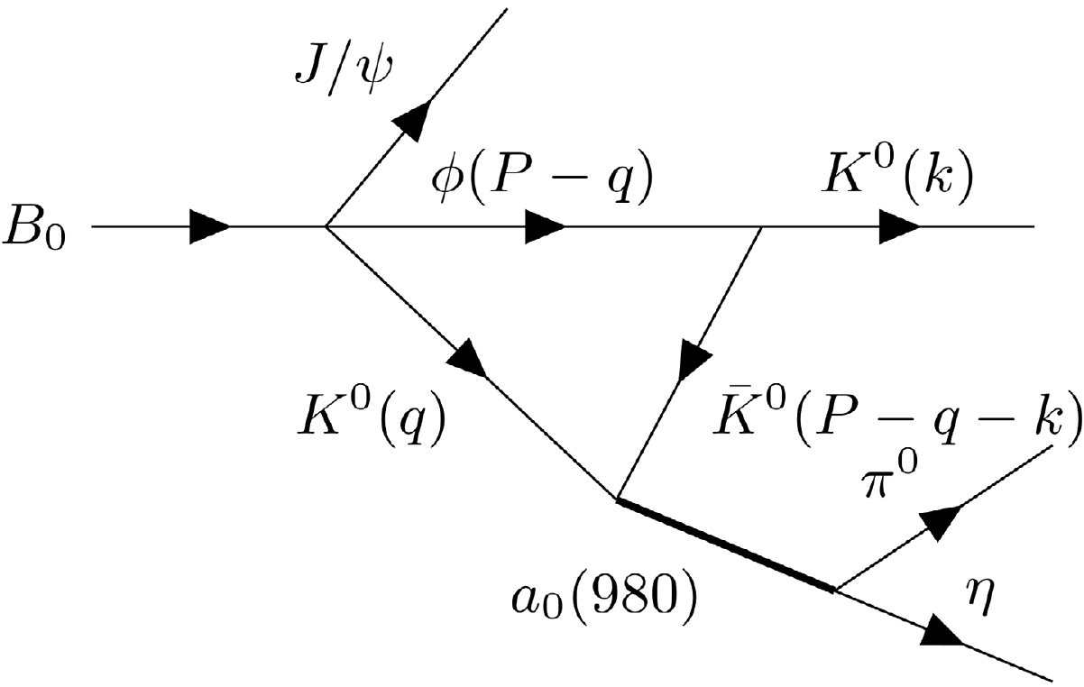

Figure 2.  Feynman diagrams of the decay process $B_0 \to $$ J/\psi K^0 a_0(980)\to J/\psi K^0\pi^0 \eta$ involving a triangle loop.

We take Fig. 1 for example to perform the following discussion, since Figs. 1 and 2 have nearly the same amplitude. Now, we want to find the position of TS in the complex-q plane, instead of evaluating the whole amplitude of a Feynman diagram including the triangle loop. Analogously to Refs. [18, 36, 37], we can use

where $q_{\rm on+}$ represents the on shell momentum of the ϕ in the center of mass frame of $ \phi K^0 $. Meanwhile, $ q_{a-} $ can be obtained by analyzing the singularity structure of the triangle loop; $ q_{a-} $ represents the on-shell $ K^0 $ momentum in the loop, antiparallel to the ϕ. $q_{\rm on+}$ and $ q_{a-} $ are given by

where s denotes the squared invariant mass of ϕ and $ K^0 $, and $ \lambda(x,y,z)=x^2+y^2+z^2-2xy-2yz-2xz $ is the Kählen function, with definitions

It is easy to realize that $ E_{K^0} $ and $ p^*_{K^0} $ are the energy and momentum of $ K^0 $ in the center of mass frame of the $ \phi K^0 $ system, and v and γ are the velocity of the $ f_0 $ and Lorentz boost factor. In addition, we can easily obtain

The three intermediate particles must be on the shell. We let the mass of $ f_0 $ be slightly larger than the sum of the masses of $ K^0 $ and $ \bar{K}^0 $; now, we can determine that the mass of $ K^0 $ is $ 497.61\ \rm M\rm eV $, the mass of $ f_0 $ is slightly larger than the sum of the masses of $ K^0 $ and $ \bar{K}^0 $, and the mass of $ f_0 $ is $ 991\ \rm{MeV} $; additionally, we can find a TS at approximately$ \sqrt{s}=1520\ \rm{MeV} $. If we use in Eq. (1) complex masses $ (M-{\rm i} \Gamma/2) $ of mesons that include widths of $ K^0 $ and $ \bar{K}^0 $, the solution of Eq. (1) is then $(1520- 10{\rm i})\ \rm{MeV}$. This solution implies that the TS has a "width" of $ 20\ \rm{MeV} $.

Here, we only focus on the $ B_0\to J/\psi\phi K^0 $ process. The decay branching ratio has been experimentally measured to be [38]

The differential decay width over the invariant mass distribution $ J/\psi \phi $ can be written as

here, $ \tilde{p}_{\phi} $ represents the momentum of the $ K^0 $ in the $ \phi K^0 $ rest frame, and $ {p_{K^0}} $ represents the momentum of the $ K^0 $ in the $ B_0 $ rest frame:

We use the polarization summation formula

and we have

where

Then, we can determine the value of the constant $ \mathcal{C} $

where the integration is performed from $ M_{\rm inv}(J/\psi\phi)_{\rm{min}} $=$ m_{J/\psi}+m_{\phi} $ to $ M_{\rm inv}(J/\psi\phi)_{\rm{max}} $=$ M_{B_0}-m_{K^0} $.

In the previous subsection, we calculated the transition strength of the decay process $ B_0\to J/\psi \phi K^0 $. Now, we calculate the contribution of the vertex $ \phi\to K^0\bar{K}^0 $. We can obtain this $ VPP $ vertex from the chiral invariant Lagrangian with local hidden symmetry given in Refs. [39–42]:

where $ \langle\rangle $ denotes the trace of the flavor SU(3) matrices, and g represents the coupling in the local hidden gauge.

The V and P in Eq. (14) are the vector meson matrix and pseudoscalar meson matrix in the SU(3) group, respectively, which are given by

Now, we can write the invariant mass distribution $ M_{\rm inv}(K^0f_0(a_0)) $ in the decay $ B_0\to J/\psi K^0 f_0 $ as

We take the first diagram of Fig. 1 and the $ B_0\to J/\psi K^0f_0 $ decay as an example and write down its amplitude as follows:

where

The $ f_0 \to K^0\bar{K}^0 $ and $ a_0\to K^0\bar{K}^0 $ vertices are obtained from the chiral unitary approach of Ref. [24] with $ g_{K^0\bar{K}^0f_0} $=2567 MeV and $ g_{K^0\bar{K}^0a_0} $=3875 MeV. $ p^{\prime}_{J/\psi} $ represents the momentum of the $ J/\psi $ in the $ B_0 $ rest frame, and $ \tilde{p}^{\prime}_{K^0}=|\vec{k}| $ represents the momentum of the $ K^0 $ in the $ K^0f_0(980) $ rest frame, where

here, $ t_T $ represents the loop amplitude:

We have

The case for $ a_0 $ production is identical, except that $ g_{K^0\bar{K}^0f_0} $ is replaced with $ g_{K^0\bar{K}^0a_0} $.

The $ K^0\bar{K}^0\to \pi^+\pi^- $ and $ K^0\bar{K}^0\to\pi^0\eta $ scattering was studied in detail in Refs. [43, 44] within the chiral unitary approach, where six channels were taken into account, including $ \pi^+\pi^- $, $ \pi^0\pi^0 $, $ K^+K^- $, $ K^0\bar{K}^0 $, $ \eta\eta $, and $ \pi^0\eta $. In the present study, we use this as input, and we shall see simultaneously both the $ f_0(980) $ (with I = 0) and $ a_0(980) $ (with I = 1) productions. Now, we can write the double differential mass distribution for the decay process $ B_0\to J/\psi K^0f_0(980)\to J/\psi K^0\pi^+\pi^- $.

For the case of $ f_0(980) $, we only have the decay $ f_0\to\pi^+\pi^- $; thus,

where $ p^{\prime\prime}_{J/\psi} $ represents the momentum of the $ J/\psi $ in the $ B_0 $ rest frame, $ \tilde p^{\prime\prime}_{K^0} $ represents the momentum of the $ K^0 $ in the $ K^0f_0(980) $ rest frame, and $ \tilde p^{\prime\prime}_{\pi} $ represents the momentum of the π in the $ \pi^+\pi^- $ rest frame:

We can obtain the amplitude of $ B_0\to J/\psi K^0f_0\to J/\psi K^0\pi^+\pi^- $:

where

and the V matrix is taken from Ref. [24]. Then, we obtain the double differential branching ratio of the $ B_0\to J/\psi K^0 f_0\to J/\psi K^0\pi^+\pi^- $ reaction:

The case for $ a_0 $ production is identical, except that $ t_{K^0\bar{K}^0,\pi^+\pi^-} $ is replaced with $ t_{K^0\bar{K}^0,\pi^0\eta} $.

Let us begin by showing in Fig. 3 the contribution of the triangle loop to the total amplitude and the triangle loop defined in Eq. (22). In order to satisfy the TS condition of Eq. (1), all intermediate particles must be on the shell; thus, the mass sum of $ K^0\bar{K}^0 $ must be smaller than that of $ f_0(a_0) $. If the mass of $ f_0(a_0) $ is too large, Eq. (1) will not be satisfied. There is hence a very narrow window of $ f_0(a_0) $ masses where the TS condition is exactly fulfilled, i.e., 995 to 999 MeV. The magnitude depends on the $ f_0(a_0) $ mass; it is independent of whether we have $ f_0 $ or $ a_0 $, since the different couplings to $ K^0\bar{K}^0 $ have been factorized out of the integral of $ t_T $. From the perspective of the above considerations, we plot the real and imaginary parts of $ t_T $, as well as the absolute value with $ M_{\rm inv}(R) $ fixed at 986, 991, and 996 MeV. We can see that the bottom one has a clear peak, because 996 MeV is in the energy window. It can be observed that Re($ t_T $) has a peak around 1518 MeV, Im($ t_T $) has a peak around 1529 MeV, and there is a peak for $ |t_T| $ around 1520 MeV. As discussed in Refs. [45, 46], the peak of the imginary part is related to the TSs, while that of the real part is related to the $ K^0\phi $ threshold. $ |t_T|=\sqrt{{\rm Re}^2(t_T)+{\rm Im}^2(t_T)} $ is between $ {\rm Re}(t_T) $ and $ {\rm Im}(t_T) $. Note that, at approximately 1520 MeV and above, the TS dominates the reaction.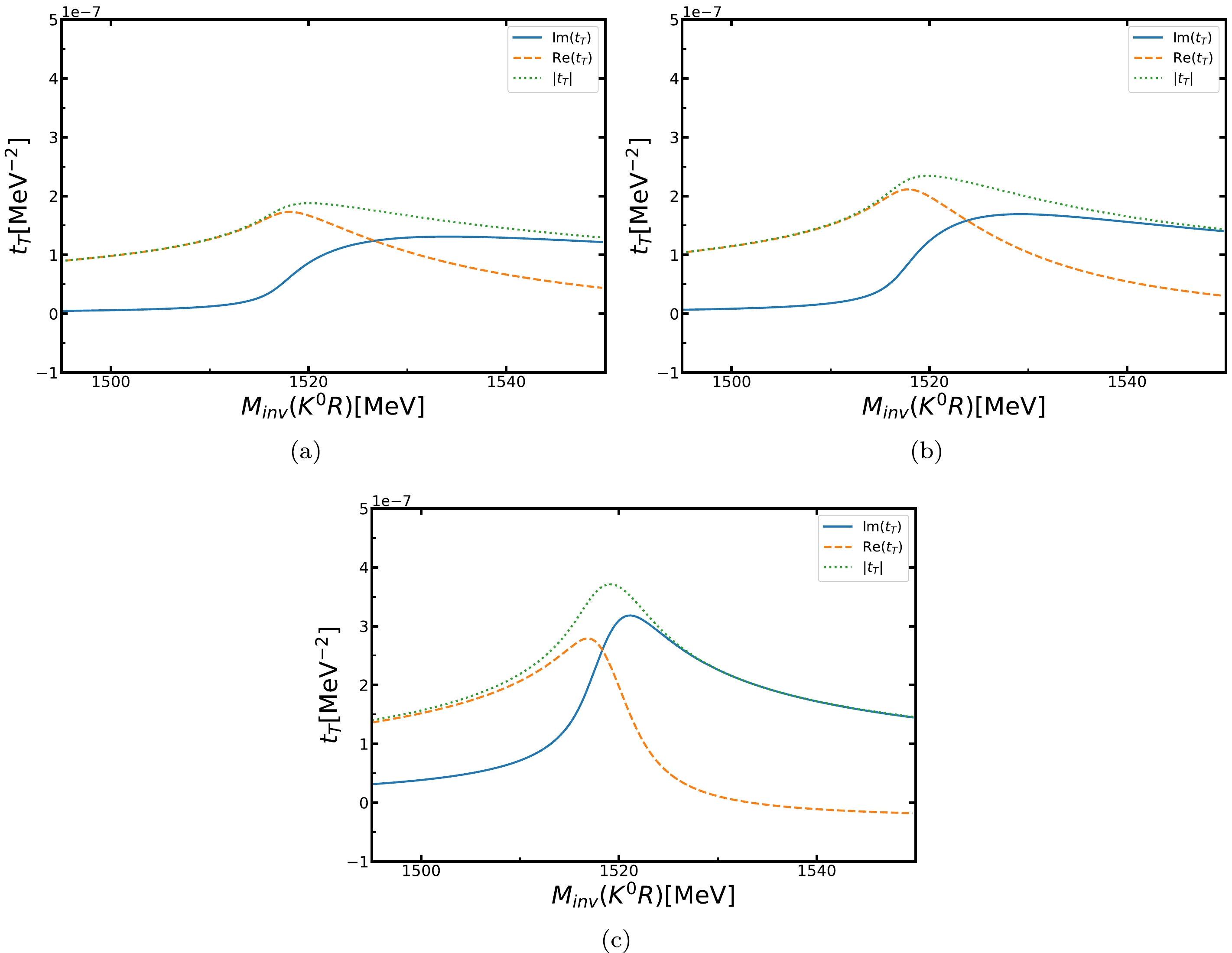

Figure 3.  (color online) Triangle amplitude $ t_T $, as a function of $ M_{\rm inv}(K^0f_0/K^0a_0) $ for (a) $ m_{f_0(a_0)} $= 986 MeV, (b) $ m_{f_0(a_0)} $= 991 MeV, and (c) $ m_{f_0(a_0)} $= 996 MeV. $ |t_T| $, Re($ t_T $), and Im($ t_T $) are plotted using green, orange, and blue curves, respectively.

Next, we show $\dfrac{1}{\Gamma_{J/\psi}}\dfrac{{\rm d}\Gamma_{B^0\to J/\psi K^0f_0(a_0)}}{{\rm d}M_{\rm{inv}}(K^0f_0/K^0a_0)}$. In Fig. 4, we plot Eq. (23) for the decay process $ B_0\to J/\psi K^0f_0(a_0) $, and we see a peak around 1520 MeV. We can obtain the branching ratio of the 3-body decay process when we integrate over $ M_{\rm inv}(K^0R) $,

Figure 4.  (color online) Differential branching ratio $\dfrac{1}{\Gamma_{B_0}}\dfrac{{\rm d}\Gamma_{B_0\to J/\psi K^0 f_0}}{{\rm d}M_{\rm inv}(K^0f_0)}$ described in Eq. (23) as a function of $ M_{\rm inv}(K^0f_0/K^0a_0) $

In the upper panel of Fig. 5, we plot Eq. (24) for the $ B_0\to J/\psi K^0\pi^+\pi^- $ decay, and similarly, in the lower panel of Fig. 5, we plot it for the $ B_0\to J/\psi K^0\pi^0\eta $ decay as a function of $ M_{\rm inv}(R) $. In both figures, we fix $ M_{\rm inv}(K^0R) $ = 1500, 1520, and 1540 MeV and vary $ M_{\rm inv}(R) $. We can see that the distribution with the highest strength is near $ M_{\rm inv}(K^0R) $ = 1520 MeV. We also observe a strong peak when $ M_{\rm inv}(\pi^+\pi^-) $ is around 980 MeV in the upper panel of Fig. 5. Similar results are shown in the lower panel of Fig. 5. We see that most of the contribution to the width Γ comes from $ M_{\rm inv}(K^0R) $=$ M_R $, and we have strong contributions for $ M_{\rm inv}(\pi^+\pi^-)\in $ [500 MeV, 990 MeV] and $ M_{\rm inv}(\pi^0\eta)\in $ [800 MeV, 990 MeV]. Therefore, when we calculate the mass distribution $\dfrac{{\rm d}\Gamma}{{\rm d}M_{\rm inv}(K^0R)}$, we restrict the integral to the limits already mentioned and perform the integration.

Figure 5.  (color online) (a) $\dfrac{{\rm d}^2\Gamma_{B_0\to J/\psi K^0f_0(980)\to\pi^+\pi^-}}{{\rm d}M_{\rm inv}(K^0f_0){\rm d}M_{\rm inv}(\pi^+\pi^-)}$ as a function of $ M_{\rm inv}(\pi^+\pi^-) $. (b) $\dfrac{{\rm d}^2\Gamma_{B_0\to J/\psi K^0a_0(980)\to J/\psi K^0\pi^0\eta}}{{\rm d}M_{\rm inv}(K^0a_0){\rm d}M_{\rm inv}(\pi^0\eta)}$ as a function of $ M_{\rm inv}(\pi^0\eta) $. The blue, orange, and green curves are obtained by setting $ M_{\rm inv}(K^0f_0)= $1500, 1520, and 1540 MeV, respectively.

We show Eq. (24) for both $ B_0\to J/\psi K^0\pi^+\pi^- $ and $ B_0\to J/\psi K^0\pi^0\eta $. When we integrate over $ M_{\rm inv}(R) $, we obtain $\dfrac{{\rm d}\Gamma}{{\rm d}M_{\rm inv}(K^0R)}$, which we show in Fig. 6. We see a clear peak of the distribution around 1520 MeV, for $ f_0 $ and $ a_0 $ production. At the same time, we observe that the peak of $ M_{\rm inv}(K^0a_0) $ is significantly lower than the peak of $ M_{\rm inv}(K^0f_0) $.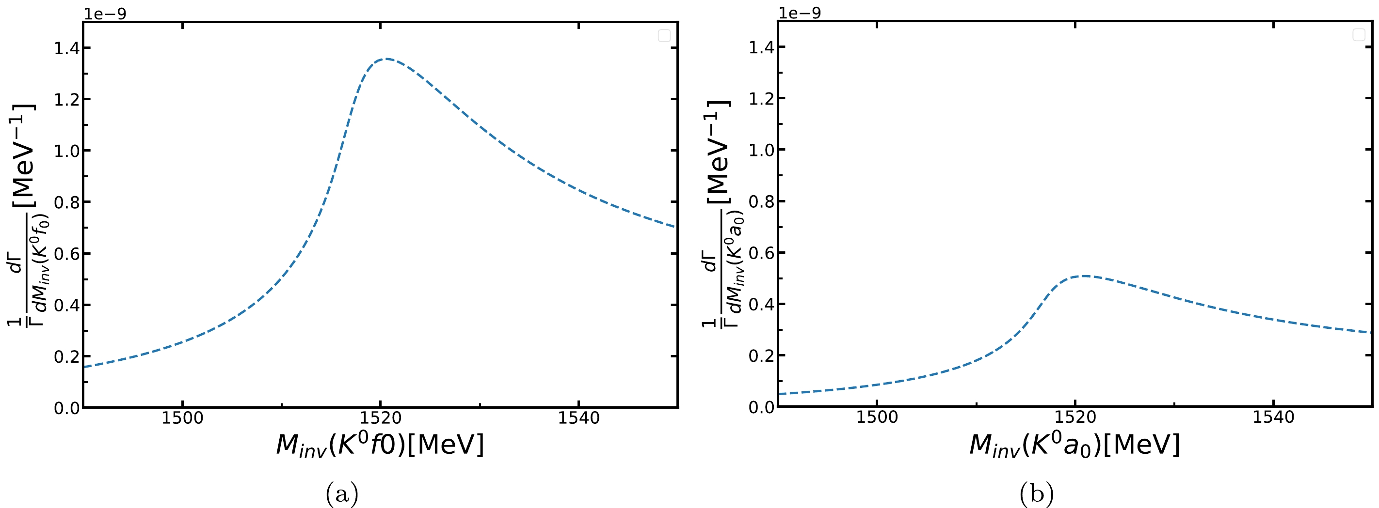

Figure 6.  (color online) (a) Differential branching ratio $\dfrac{{\rm d}\Gamma_{B_0\to J/\psi K^0f_0(980)\to J/\psi K^0\pi^+\pi^-}}{{\rm d}M_{\rm inv}(K^0f_0)}$. (b) Branching ratio $\dfrac{{\rm d}\Gamma_{B_0\to J/\psi K^0f_0(980)\to J/\psi K^0\pi^+\pi^-}}{{\rm d}M_{\rm inv}(K^0a_0)}$ described in Eq. (24) as a function of $ M_{\rm inv}(K^0f_0/K^0a_0) $

By integrating $\dfrac{{\rm d}\Gamma}{{\rm d}M_{\rm inv}(K^0f_0)}$ and $\dfrac{{\rm d}\Gamma}{{\rm d}M_{\rm inv}(K^0a_0)}$ over the $ M_{\rm inv}(K^0f_0) $($ M_{\rm inv}(K^0a_0) $) masses in Fig. 6, we obtain the branching fractions:

We performed calculations for the reactions $ B_0\to J/\psi K^0 f_0(980)(a_0(980)) $ and showed that they develop a TS for an invariant mass of 1520 MeV in $ (K^0R) $. This TS shows up as a peak in the invariant mass distribution of these pairs with an apparent width of approximately 20 MeV. We applied the experimental data of the branching ratio of the decay $ B_0\to J/\psi K^0 f_0(980)(a_0(980)) $ to determine the coupling strength of the $B_0\to J/\psi K^0 f_0(980)\times (a_0(980))$ vertex.

We evaluated $\dfrac{{\rm d}^2\Gamma_{\rm total}}{{\rm d}M_{\rm inv}(K^0R){\rm d}M_{\rm inv}(R)}$ and observed clear peaks in the distributions $ M_{\rm inv}(\pi^+\pi^-) $($ M_{\rm inv}(\pi^0\eta) $), clearly showing the $ f_0(a_0) $ shapes. With integration over $ M_{\rm inv}(R) $, these distributions exhibited a clear peak for $ M_{\rm inv}(K^0R) $ around 1520 MeV.

This peak is a result of the singularity of the triangle and may be misidentified with resonance when the experiment is completed. In this sense, the present work should serve as a warning not to treat this peak as resonance when it is seen in future experiments. It is important to discover new conditions about TSs and to allow for this possibility when experimentally observed peaks can avoid associating these peaks with resonance. The value of this work lies in identifying a TS for a suitable reaction and then preparing the results and research to interpret the peak correctly when it is observed.