


 Abstract
 HTML
HTML Reference
 Related
 PDF
PDF


-
Cosmological surveys over decades enable us to draw a picture of modern cosmology based on the ΛCDM baseline model, except with several fundamental puzzles such as the nature of dark matter (DM). Among various efforts to detect DM, 21-cm cosmology [1] as a probe for the spin flipping of the ground-state hydrogen atom of baryon gas during the dark ages provides a new way to search for DM in a low velocity region. Because the brightness temperature
$ T_{21} $ of the hydrogen 21-cm line is tied to baryon temperature$ T_b $ , measurement of$ T_{21} $ sheds light on the DM-baryon interaction [2−4], which can affect$ T_b $ . Recently, the EDGES experiment reported the first measurement of the sky-averaged value [5]$ \begin{eqnarray} { } \left<T_{21}\right>= -500^{+ 200}_{- 500}\; \rm{mK}, \end{eqnarray} $

(1) at redshift
$ z\approx 17 $ , which deviates from the prediction of ΛCDM with a significance of$ \sim 3.8\; \sigma $ .1 Because this signal strongly favors the DM-baryon interaction, it is natural to wonder what type of DM model and with what type of DM-baryon interaction within which DM mass range can cool down the baryon gas to explain the EDGES data.Several studies have advocated the Coulomb-like interaction between DM and baryons as a solution [8−18] to the observed signal. If this is the case, a massless or light force carrier ω is essential, implying that such DM is actually freeze-in.
2 The freeze-in DM-baryon elastic scattering cross section scales as$ \sim \upsilon^{-4}_{\rm{rel}} $ , where$ \upsilon_{\rm{rel}} $ is the relative velocity of interacting particles. This velocity-dependent behavior significantly amplifies the effect on$ T_b $ at low velocities such as$ \upsilon_{\rm{rel}}\sim 10^{-6} $ at the redshift$ z\approx 17 $ , compared to those at relatively higher$ \upsilon_{\rm{rel}} $ , such as in DM direct detection experiments (with$ \upsilon_{\rm{rel}}\sim 10^{-3} $ ) or the early Universe (with$ \upsilon_{\rm{rel}}\sim 0.1-1 $ ).3 In other words, Coulomb-like interactions naturally provide a large gap between the cross sections related to the signal and the aforementioned constraints among others. Nevertheless, previous studies have indicated that such a gap remains inadequate in simple DM models.In this study, we instead investigate the freeze-in DM scenario through a model-independent survey. To be concrete, we focus on freeze-in DM interacting with the charged particles of baryon gas, namely, electrons and protons in the standard model (SM). For light force carrier masses heavier than the eV scale, as considered here, the most relevant constraints from DM direct detection, such as DM-electron (e) scattering [20−27] and DM-proton (p) scattering [28−33], early cosmology, such as big bang nucleosynthesis (BBN) [34] and cosmic microwave background (CMB) [4, 12, 35−37], stellar cooling [38−41], large-scale structure (LSS) [42, 43], and colliders [44, 45], can be divided into model-dependent and model-independent catalogs (see Fig. 1 for an overview).
4 Among these constraints, the stellar cooling bounds are the most stringent in the parameter regions where they are present. Because the stellar cooling bounds can be promoted to model-independent ones, we are able to discover whether a viable parameter space exists after the most important model-independent constraints are imposed. A surviving region, if any, is useful for DM model builders not familiar with 21-cm cosmology.
Figure 1. (color online) Overview of the most relevant constraints on freeze-in DM with eV-keV scale force carrier(s) divided into model-dependent (top) and model-independent (bottom) ones. The most stringent stellar cooling bounds can be promoted to be mode-independent.
This paper has the following structure: In Sec. II, we introduce two different descriptions of the scattering cross sections used by EDGES 21-cm signal analysis and DM direct detection experiments. Sec. III is devoted to the Boltzmann equations that govern the temperature evolution of both DM and baryon fluid after kinetic decoupling, where one- and two-component DM are considered in Sec. III.A and Sec. III.B, respectively. By numerically solving the Boltzmann equations, we analyze the parameter space with respect to the EDGES signal in the sub-GeV DM mass range for the one- and two-component cases in Sec. IV.A and Sec. IV.B, respectively, and identify the physical implications to simplified freeze-in DM models. Finally, we conclude in Sec. V.
-
The cross sections
$ \hat{\sigma}^{I} $ used by the EDGES signal analysis are given by$ \begin{equation} { } \sigma^{I}_{T}=\hat{\sigma}^{I}\upsilon^{-4}_{\rm{rel}}, \end{equation} $

(2) where
$ I=\{e, p\} $ refers to a component of baryon gas contributing to the DM-baryon scattering, and$ \sigma^{I}_{T} $ is the so-called momentum-transfer cross section defined as [42]$ \begin{eqnarray} { } \sigma^{I}_{T}=\int {\rm d}\Omega (1-\cos\theta)\frac{{\rm d}\sigma^{I}}{{\rm d}\Omega}, \end{eqnarray} $

(3) where
${\rm d}\sigma^{I}/{\rm d}\Omega$ is the differential cross section, and θ is the scattering angle.As noted in previous studies, for example, [11],
$ \hat{\sigma}^{I} $ are different from the cross sections$ \bar{\sigma}^{I} $ used by DM direct detection experiments, defined as$ \begin{eqnarray} { } \frac{{\rm d}\sigma^{I}}{{\rm d}\Omega}=\frac{\bar{\sigma}^{I}}{4\pi}\bigg| F_{\chi}(q^{2})\bigg|^{2} \bigg| f(q^{2})\bigg|^{2}, \end{eqnarray} $

(4) where
$ F_{\chi}(q^{2})\sim 1/q^{2} $ is the DM form factor, and$ f(q^{2})\approx 1 $ is the target form factor. Substituting Eq. (4) into Eq. (3) gives [11]$ \begin{eqnarray} { } \bar{\sigma}^{I}\approx 8\xi^{-1}_{I}\left(\frac{\mu_{I}}{q_I}\right)^{4}\hat{\sigma}^{I}, \end{eqnarray} $

(5) where
$ \mu_{I} $ is the DM-I reduced mass,$ q_{I} $ is the typical moment transfer in the relevant scattering process, and$ \xi_{I} $ is the logarithm term$ \begin{eqnarray} { } \xi_{I}\approx\log\left(\frac{4\mu^{2}_{I}\upsilon^{2}_{\rm{rel}}}{m_{\omega}^{2}}\right). \end{eqnarray} $

(6) Here,
$ m_{\omega} $ is the force carrier mass.For comparison with DM direct detection limits, we must convert
$ \hat{\sigma}^{I} $ obtained from the EDGES signal into$ \bar{\sigma}^{I} $ using Eq. (5), where the explicit values of$ q_{I} $ and$ \xi_{I} $ are DM experiment-relevant. In the DM mass range$ m_{\chi}\sim 1-10^{3} $ MeV, the most stringent limits can be placed as follows: For the DM-e cross section$ \bar{\sigma}^e $ , we pay attention to both the SENSEI [25] and XENON [27] limits, which are able to constrain most of the mass ranges. In these experiments,$ q_{e}\approx \alpha m_{e} $ , as in [11], where α is the fine structure constant, and the value of$ \xi_{I} $ is determined by$ m_{\omega} $ requiring$ m_{\omega}\leq 10^{-6}\mu_{I} $ in the red shift region$ z \sim 10-10^{3} $ and the relative velocity$ \upsilon_{\rm{rel}}\sim 10^{-3} $ at these DM direct detection experiments. For the DM-p cross section$ \bar{\sigma}^p $ , which is assumed to be spin-dependent, we consider the XENON1T [31] limit to constrain$ m_{\chi} $ down to$ \sim $ 80 MeV. At the XENON1T experiment, the moment transfer$ q_{p}\approx \sqrt{2m_{p}E_{R}}\sim 1.0-2.0 $ MeV [31], where$ E_{R}\sim 1-2 $ keV is the recoil energy. -
In this section, we derive the Boltzmann equations that govern the temperature evolution of both DM and baryon gas as perfect fluids after kinetic decoupling. The DM-baryon interaction, which is non-relativistic, yields two main effects [2−4]: a transfer of heating and a change in relative velocity between the two fluids.
-
With DM being a single component, the transfer of heating is described by the heating terms
$ Q_{b, \chi} $ , which respect energy conservation, whereas the change in relative velocity between DM and baryon fluid is characterized by the drag term D. In the situation where the DM particle χ simultaneously interacts with the different components I of the baryon fluid, the above factors are given by$ \begin{aligned}[b] D=&-\dot{V}_{\chi b}=\sum_{I}\frac{(\rho_{\chi}+\rho_{b})}{m_{\chi}+m_{I}}\frac{\rho_I}{\rho_{b}} \int {\rm d}^{3}\mathbf{v}_{\chi}f_{\chi} \int {\rm d}^{3}\mathbf{v}_{I}f_{I}\\&\times\left[\sigma^{I}_{T}\mid\mathbf{v}_{\chi}-\mathbf{v}_{I}\mid \frac{\mathbf{V}_{\chi b}}{V_{\chi b}}\cdot(\mathbf{v}_{\chi}-\mathbf{v}_{I})\right], \end{aligned} $

$ \begin{aligned}[b] \dot{Q}_{b}=&\sum_{I}\frac{\rho_{\chi} x_{I}m_{I}}{m_{\chi}+m_{I}} \int {\rm d}^{3}\mathbf{v}_{\chi}f_{\chi} \int {\rm d}^{3}\mathbf{v}_{I}f_{I}\\&\times\left[\sigma^{I}_{T}\mid\mathbf{v}_{\chi}-\mathbf{v}_{I}\mid\mathbf{v}_{\rm{CM}}\cdot (\mathbf{v}_{I}-\mathbf{v}_{\chi})\right], \\ \dot{Q}_{\chi}=&\sum_{I}\frac{\rho_{I}m_{\chi}}{m_{\chi}+m_{I}} \int {\rm d}^{3}\mathbf{v}_{\chi}f_{\chi} \int {\rm d}^{3}\mathbf{v}_{I}f_{I}\\&\times\left[\sigma^{I}_{T}\mid\mathbf{v}_{\chi}-\mathbf{v}_{I}\mid\mathbf{v}_{\rm{CM}}\cdot (\mathbf{v}_{\chi}-\mathbf{v}_{I})\right], \end{aligned} $

(7) where the "dot" refers to the derivative over time, the sum is over e and p,
$ \sigma^{I}_{T} $ is given by Eq. (2),$ \rho_b $ ,$ \rho_I $ , and$ \rho_{\chi} $ are the baryon, I-component of baryon gas, and DM density, respectively,$ f_{\chi} $ and$ f_{I} $ are the phase space density of DM and the I-component particle, respectively,$ x_{I} $ is the fraction of the I-component number density, and$ \mathbf{v}_{i} $ and$ \mathbf{V}_{j} $ represent the velocity of particle i and fluid j, respectively. Under this notation,$ \mathbf{v}_{\rm{CM}}=(m_{I}\mathbf{v}_{I}+m_{\chi}\mathbf{v}_{\chi})/(m_{I}+m_{\chi}) $ is the center-of-mass velocity, while$ V_{\chi b}=\mid \mathbf{V}_{\chi b}\mid= \mid \mathbf{V}_{\chi}-\mathbf{V}_{b}\mid $ is the relative velocity of the two relevant fluids.Inserting Eq. (2) into Eq. (7) and integrating over the particle velocities
$ \mathbf{v}_{\chi} $ and$ \mathbf{v}_{I} $ give rise to the explicit expressions$ \begin{aligned}[b] D=&\sum_{I}\hat{\sigma}^{I}\frac{(\rho_{\chi}+\rho_{b})}{m_{\chi}+m_{I}}\frac{\rho_I}{\rho_{b}}\frac{F(r_{I})}{V^{2}_{\chi b}}, \\ \dot{Q}_{b}=&\sum_{I}\frac{\rho_{\chi} x_{I}m_{I}}{(m_{\chi}+m_{I})^{2}}\frac{\hat{\sigma}^{I}}{u_{th,I}}\left[\sqrt{\frac{2}{\pi}}\frac{{\rm e}^{-r^{2}_{I}/2}}{u^{2}_{th,I}}(T_{\chi}-T_{b})+m_{\chi}\frac{F(r_{I})}{r_{I}}\right], \\ \dot{Q}_{\chi}=&\sum_{I}\frac{\rho_{I}m_{\chi}}{(m_{\chi}+m_{I})^{2}}\frac{\hat{\sigma}^{I}}{u_{th,I}}\left[\sqrt{\frac{2}{\pi}}\frac{{\rm e}^{-r^{2}_{I}/2}}{u^{2}_{th,I}}(T_{b}-T_{\chi})+m_{I}\frac{F(r_{I})}{r_{I}}\right], \end{aligned} $

(8) where
$F(r_{I})={\rm erf}(r_{I}/\sqrt{2})-\sqrt{\dfrac{2}{\pi}}r_{I}{\rm e}^{-r_{I}^{2}/2}$ with$ r_{I}= \frac{V_{\chi b}}{u_{th,I}}, \quad u_{th,I}=\sqrt{\frac{T_{b}}{m_{I}}+\frac{T_{\chi}}{m_{\chi}}}. $

(9) Considering the collision terms, we obtain the complete Boltzmann equations [2] for the temperatures of DM and baryon fluid:
$ \begin{aligned}[b] \frac{{\rm d}T_{\chi}}{{\rm d}a}=& -2 \frac{T_{\chi}}{a} +\frac{2\dot{Q}_{\chi}}{3 aH}, \\ \frac{{\rm d}T_{b}}{{\rm d}a}=& -2 \frac{T_{b}}{a} + \frac{\Gamma_{C}}{aH}(T_{\gamma}-T_{b})+ \frac{2\dot{Q}_{b}}{3aH}, \\ \frac{{\rm d} V_{\chi b}}{{\rm d}a}=& - \frac{V_{\chi b}}{a} - \frac{D}{aH}, \\ \frac{{\rm d} x_{e}}{{\rm d}a}=& -\frac{\mathcal{C}}{aH}\left[n_{H}\mathcal{A}_{B}x^{2}_{e}-4(1-x_{e})\mathcal{B}_{B} {\rm e}^{3E_{0}/4T_{\gamma}}\right], \end{aligned} $

(10) where H is the Hubble parameter,
$ a=(1+z)^{-1} $ is the scale factor,$ T_{\gamma}(z)=T_{0}(1+z) $ is the CMB temperature with a current value of$ T_{0}=2.725 $ K,$ \Gamma_{C} $ is the Compton interaction rate,$ \mathcal{C} $ is the Peebles factor [48],$ E_0 $ is the hydrogen ground energy, and$ \mathcal{A}_{B} $ and$ \mathcal{B}_{B} $ [49, 50] are the effective recombination coefficient and photoionization rate, respectively. As shown in Eq. (10), a decrease in$ T_b $ toward a low red shift requires a negative$ \dot{Q}_b $ , which is more easily obtained in the small$ m_{\chi} $ range, as shown in Eq. (8). It is easy to verify that the derived analytical results in Eqs. (7)−(10) reduce to those of Refs. [2−4] by taking I as e or p.We numerically solve Eq. (10) via the following initial conditions:
$ \begin{aligned}[b] T_{\chi}(z_{\rm{kin}})=&0, \\ T_{b}(z_{\rm{kin}})=&T_{\gamma}(z_{\rm{kin}}), \\ x_{e}(z_{\rm{kin}})\approx& 0.08, \end{aligned} $

(11) at kinetic decoupling with the redshift
$ z_{\rm{kin}}=1010 $ . -
Now, we consider DM composed of two different components
$ \chi_{i} $ , with$ i= $ 1−2. Without loss of generality, we couple the$ \chi_{1} $ - and$ \chi_{2} $ -components to the electrons and protons of baryon fluid, respectively. As in the one-component case, there is only a baryon fluid velocity$ \mathbf{V}_b $ ; however, there are conversely two$ \chi_i $ fluid velocities$ \mathbf{V}_{\chi_{i}} $ . As a result, in the two-component case, we have two relative fluid velocities$ V_{\chi_{i}b}=\mid \mathbf{V}_{\chi_{i}}-\mathbf{V}_{b}\mid $ , two drag terms$ D_{i}=-\dot{V}_{\chi_{i} b} $ , and four heating terms$ Q_{b_{i}} $ and$ Q_{\chi_{i}} $ .In the same spirit of Eq. (7), we have the explicit forms of
$ D_1 $ ,$ Q_{\chi_{1}} $ , and$ Q_{b_{1}} $ as follows:$ \begin{aligned}[b] D_{1}=&\hat{\sigma}^{e}\frac{\rho_{\chi_{1}}+\rho_{e}}{m_{\chi_{1}}+m_{e}}\frac{F(r_{e})}{V^{2}_{\chi_{1}b}}+ \hat{\sigma}^{p}\frac{\rho_{\chi_{2}}}{m_{\chi_{2}}+m_{p}}\frac{F(r_{p})}{V^{2}_{\chi_{2}b}}, \\ \dot{Q}_{b_{1}}=&\frac{\rho_{\chi_{1}} x_{e}m_{e}}{(m_{\chi_{1}}+m_{e})^{2}} \frac{\hat{\sigma}^{e}}{u_{th, e}} \left[\sqrt{\frac{2}{\pi}}\frac{{\rm e}^{-r^{2}_{e}/2}}{u^{2}_{th,e}}(T_{\chi_{1}}-T_{b})+m_{\chi_{1}}\frac{F(r_{e})}{r_{e}}\right], \\ \dot{Q}_{\chi_{1}}=&\frac{\rho_{e}m_{\chi_{1}}}{(m_{\chi_{1}}+m_{e})^{2}} \frac{\hat{\sigma}^{e}}{u_{th,e}} \left[\sqrt{\frac{2}{\pi}}\frac{{\rm e}^{-r^{2}_{e}/2}}{u^{2}_{th,e}}(T_{b}-T_{\chi_{1}})+m_{e}\frac{F(r_{e})}{r_{e}}\right], \end{aligned} $

(12) with
$\begin{aligned}[b] r_{e}=& \frac{V_{\chi_{1}b}}{u_{th,e}},\\ u_{th,e}=&\sqrt{\frac{T_{b}}{m_{e}}+\frac{T_{\chi_{1}}}{m_{\chi_{1}}}}. \end{aligned}$

(13) The forms of
$ D_2 $ ,$ Q_{b_{2}} $ , and$ Q_{\chi_{2}} $ are obtained by simultaneously replacing$ 1\rightarrow 2 $ and$ e\rightarrow p $ in Eqs. (12) and (13). Note that for$ D_1 $ in Eq. (12), the second term arises from the$ \chi_{2} $ -baryon interaction, regardless of whether the$ \chi_{1} $ -baryon interaction is present, and vice versa for$ D_2 $ . This is one of the key features that differ from Eq. (8) in the previous case.Equipped with Eq. (12), the Boltzmann equations in Eq. (10) are replaced by
$ \begin{aligned}[b] \frac{{\rm d}T_{\chi_{i}}}{{\rm d}a}=& -2 \frac{T_{\chi_{i}}}{a} +\frac{2\dot{Q}_{\chi_{i}}}{3 aH}, \\ \frac{{\rm d}T_{b}}{{\rm d}a}=& -2 \frac{T_{b}}{a} + \frac{\Gamma_{C}}{aH}(T_{\gamma}-T_{b})+ \frac{2\sum_{i}\dot{Q}_{bi}}{3aH}, \\ \frac{{\rm d}V_{\chi_{i} b}}{{\rm d}a}=& - \frac{V_{\chi_{i} b}}{a} - \frac{D_{i}}{aH}, \\ \frac{{\rm d}x_{e}}{{\rm d}a}=& -\frac{\mathcal{C}}{aH}\left[n_{H}\mathcal{A}_{B}x^{2}_{e}-4(1-x_{e})\mathcal{B}_{B}{\rm e}^{3E_{0}/4T_{\gamma}}\right], \end{aligned} $

(14) where
$ T_{\chi_{i}} $ refers to the separate temperatures of$ \chi_i $ fluids.Instead of Eq. (11), the initial conditions for Eq. (14) are given by
$ \begin{aligned}[b] T_{\chi_{i}}(z_{\rm{kin}})=&0, \\ T_{b}(z_{\rm{kin}})=&T_{\gamma}(z_{\rm{kin}}), \\ x_{e}(z_{\rm{kin}})\approx& 0.08. \end{aligned} $

(15) As one derives
$ T_{21} $ from the Boltzmann equations either in Eq. (10) or (14) with an initial value of$ V_{\chi b}(z_{\rm{kin}})=V_{\chi b,0} $ , it is actually described by the Maxwell-Boltzmann distribution$ \begin{eqnarray} { } \mathcal{P}(V_{\chi b,0})=\frac{4\pi }{(2\pi V^{2}_{\rm{rms}}/3)^{3/2}}V^{2}_{\chi b,0} {\rm e}^{-3V^{2}_{\chi b,0}/(2V^{2}_{\rm{rms}})}, \end{eqnarray} $

(16) with
$ V_{\rm{rms}}\approx 29 $ km/s at kinetic decoupling. Therefore, the final value of$ T_{21} $ should be sky-averaged as follows:$ \begin{aligned}[b] { } \left<T_{21}\right>= \left\{ \begin{array}{lcl} \displaystyle\int {\rm d} V_{\chi b} \mathcal{P}(V_{\chi b,0})T_{21}(V_{\chi b,0}), \; \; \; \; \; \; \; \; \; \; \; \; \; \; \; \; \; \; \; \; \; \; \; \; \; \; \; \; \; \; \; \; \rm{one-component},\\ \displaystyle\int {\rm d} V_{\chi_{1} b} {\rm d} V_{\chi_{2} b}\mathcal{P}(V_{\chi_{1} b,0})\mathcal{P}(V_{\chi_{2} b,0})T_{21}(V_{\chi_{1} b,0}, V_{\chi_{2} b,0}), \; \; \rm{two-component},\\ \end{array}\right. \end{aligned} $ 
(17) where each
$ V_{\chi_{i} b,0} $ in the two-component case satisfies the same Maxwell-Boltzmann distribution in Eq. (16). The thermal average in Eq. (17) is necessary to eliminate statistical errors, even though this demands a larger computational source to handle numerical analysis in the next section. -
Let us now discuss the parameter spaces that can explain the observed EDGES 21-cm signal. We divide our study into two representative cases, as shown in Table 1, where the one-component DM contains only a force carrier (ω) and the two-component DM contains two different force carriers
$ \omega_{i} $ . In the first case, it is sufficient to introduce the DM mass$ m_{\chi} $ and two cross sections$ \hat{\sigma}^{e} $ and$ \hat{\sigma}^{p} $ to parameterize the parameter space, whereas in the second case, we introduce two DM masses$ m_{\chi_{i}} $ , two cross sections as above, and a new parameter δ,Pattern of the DM-baryon interaction Parameters one-component 
$m_{\chi},\;\hat\sigma _e,\; \hat \sigma_p$ 

two-component 
$m_{\chi i},\;\hat\sigma _e,\; \hat \sigma_p ,\;\delta$ 

Table 1. Two DM scenarios considered. In the one-component case, DM
$ \chi $ is assumed to couple to both$ e $ and$ p $ via light force carries$ \omega $ with the mass in the range eV-keV. Together with$ m_{\chi} $ , the two scattering cross sections$ \sigma^{I}_{T} $ with$ I=\{e,p\} $ , which scale as in Eq. (2), are used as the input parameters. Likewise, in the two-component case, DM is composed of two different fields$ \chi_{1} $ and$ \chi_{2} $ coupled to$ e $ via$ \omega_{1} $ and$ p $ via$ \omega_{2} $ , respectively, with the masses of two force carries in the range eV-keV, two cross sections$ \sigma^{I}_{T} $ scaled as in Eq. (2), and a fraction of DM energy density denoted by$ \delta $ $ \begin{aligned}[b] \rho_{1}= \delta\rho_{\rm{CDM}}, \quad \rho_{2}= (1-\delta)\rho_{\rm{CDM}}, \end{aligned} $

(18) to describe the fraction of each DM component energy density, where
$ \rho_{\rm{CDM}}\approx 0.3 $ GeV$ / $ cm$ ^{3} $ is the observed cold DM energy density. -
Figure 2 shows the parameter space of the one-component DM model, which satisfies
$ -500 \leq T_{21}\leq -300 $ mK, as reported by the EDGES experiment with$ m_{\omega}=1 $ eV. Note that the mass range of$ m_{\omega} $ allowed by the requirement$ m_{\omega}\leq 10^{-6}\mu_{I} $ in the entire DM range$ m_{\chi}\sim 1-10^{3} $ MeV for both$ I=e $ and$ I=p $ is, at most, of the order of the$ \sim $ eV scale. For each sample in this figure, we choose$ q_{p}\approx 2 $ MeV when converting$ \hat{\sigma}^{p} $ into$ \bar{\sigma}^{p} $ in Eq. (5), which results in an uncertainty of the order of$ \sim $ a few times in$ \bar{\sigma}^{p} $ in a certain DM mass range.
Figure 2. (color online) Samples yielding
$ -500 \leq \left<T_{21}\right> \leq -300 $ mK, reported by the EDGES experiment in one-component DM with$ m_{\omega}=1 $ eV, which are projected onto the plot of$ m_{\chi}-\bar{\sigma}^{e} $ ($ \mathbf{top} $ ) and$ m_{\chi}-\bar{\sigma}^{p} $ ($ \mathbf{bottom} $ ). For comparison, we also show the SENSEI limit (black) [25] on DM-e scattering, the XENON1T limit on DM-e (gray) [27] and spin-dependent DM-p (dotted-dashed) [31] scattering, the CMB limit (dashed) [37] on DM-p scattering, and the stellar cooling limits [40] (purple). Samples above the limits are excluded. See text for details.To identify whether a constraint is model-independent or model-dependent, we emphasize that behind the cross sections
$ \begin{eqnarray} { } \bar{\sigma}^{I}\approx \frac{16\pi\alpha_{I}\alpha_{\chi}}{q^{4}_{I}}\mu^{2}_{I}, \end{eqnarray} $

(19) there are two structure constants
$ \alpha_{I} $ and$ \alpha_{\chi} $ with respect to the ω-SM and ω-DM systems, respectively (see Fig. 1 for a sketch). Let us individually examine the constraints mentioned in Sec. I.● DM direct detection. These limits are model-independent. In the mass range
$ m_{\chi}\sim 1-10^{3} $ MeV, the most stringent limits on$ \bar{\sigma}^{e} $ arise from SENSEI (black) [25] and XENON1T (gray) [27]), while an up-to-date spin-dependent limit on$ \bar{\sigma}^{p} $ originates from XENON1T (dotted-dashed) [31].● BBN constraint. BBN places a constraint on the effective number of neutrinos
$ N_{\rm{eff}} $ due to the relativistic effect [34] of light ω. Because the effect on$ N_{\rm{eff}} $ is determined by the mediator energy density$ \rho_{\omega} $ , the BBN constraint is model-dependent.● CMB constraint. Similar to the BBN constraint, the CMB constraint on
$ N_{\rm{eff}} $ [34] is also model-dependent. Apart from$ N_{\rm{eff}} $ , measurements on CMB anisotropy offer another method to precisely constrain DM-baryon interactions. A model-independent upper bound on$ \bar{\sigma}^{p} $ (dashed) can be found in [37] without the DM-e interaction (that is,$ \alpha_{e}=0 $ ).● Supernova 1987A (SN1987A). The energy loss of SN1987A to both the χ and ω particles places an upper bound dependent on
$ \alpha_{\chi} $ ,$ \alpha_{e} $ , and$ \alpha_{p} $ . To date, the available SN1987A bounds in literature [39, 40] only apply to specific DM models such as the dark photon DM model with$ \alpha_{e}\sim \alpha_{p} $ .● Stellar cooling. In a stellar object such as the sun, horizontal-branch stars, or red-giants (RG), the energy loss to light ω particles with the mass scale
$ m_{\omega} $ smaller than keV [40, 41] can be significant. By turning off$ \alpha_{p} $ ($ \alpha_{e} $ ), the stellar cooling bound5 on$ \alpha_{e} $ ($ \alpha_{p} $ ) [40] can be promoted to model-independent constraints with the help of a rational bound$ \alpha_{\chi}\leq 1 $ , as shown in the plot of$ m_{\chi}-\bar{\sigma}^{e}(\bar{\sigma}^{p}) $ in purple.● LSS. This imposes a rough upper bound [42] on the effect of DM self interaction controlled by
$ \alpha_{\chi} $ , which can be satisfied by$ \alpha_{\chi}\leq 1 $ .● Colliders. The constraints on
$ \alpha_e $ by lepton colliders, such as the LEP, and on$ \alpha_p $ by hadron colliders, such as the LHC, are obviously less competitive than the stellar cooling bounds in the parameter regions considered.Compared to DM direct detection, BBN, CMB, and collider limits, the stellar cooling bounds are used for estimates of the magnitudes of structure constants at best. Even so, they are the most stringent constraints in the parameter regions where they are present. This point can be easily verified by choosing an explicit value of
$ \alpha_{e} $ or$ \alpha_{p} $ below the stellar cooling bounds.Figure 2 reveals two key points. The first is that the parameter space for the simplified one-component DM models, where either
$ \alpha_{e} $ or$ \alpha_{p} $ is absent, corresponds to parameter regions with negligible$ \bar{\sigma}^{e} $ or$ \bar{\sigma}^{p} $ , respectively. To manifest this, we label the samples in the case of tiny$ \bar{\sigma}^{e} $ with "$ \star $ ." Below the stellar cooling bound on$ \alpha_e $ in the$ \mathbf{top} $ plot, these star points are excluded by the stellar cooling bound on$ \alpha_p $ in the$ \mathbf{bottom} $ plot, and vice versa. This result applies to the simplified one-component freeze-in DM model with the light force carrier as gauged$ L_{e}-L_{\mu} $ or$ L_{e}-L_{\tau} $ [51−54]. The second point is that when$ \alpha_{e} $ and$ \alpha_{p} $ are present and their contributions to$ \left<T_{21}\right> $ are comparable, the samples are clearly excluded by the stellar cooling bounds if not by the DM direct detection limits, etc. This result applies to the simplified one-component freeze-in DM model with the light force carrier as gauged$ B-L $ [54−57] with$ \alpha_{e}/\alpha_{p}\sim 1 $ , a dark photon [58−60] with$ \alpha_{e}/\alpha_{p}\sim 1 $ , or an axion-like particle (ALP)6 with various ratios of$ \alpha_{e}/\alpha_{p} $ .The exclusion is robust because
$ i) $ when both$ \alpha_{e} $ and$ \alpha_{p} $ are present, the stellar cooling bounds are still valid as an estimate of the order of magnitudes, and$ ii) $ the magnitudes of the cross sections for the samples in Fig. 2 change at most by one-to-two orders when the value of$ m_{\omega} $ is adjusted in the allowed mass range of 1-$ 10^3 $ eV. These results partially explain the motivation for proposing the mini-charged DM model, as mentioned in the Introduction, where the stringent stellar cooling bounds no longer exist in the DM mass range with$ m_{\chi} $ above the MeV scale. -
Similar to the one-component DM case, we now present the parameter space of two-component DM, which can explain the EDGES data. In this situation,
$ \bar{\sigma}^{I} $ depends on two different masses$ m_{\omega_{i}} $ , as opposed to one in one-component DM. Therefore, there are more options on$ m_{\omega_{i}} $ to satisfy the requirements$ m_{\omega_{1}}\leq 10^{-6}\mu_{e} $ and$ m_{\omega_{2}}\leq 10^{-6}\mu_{p} $ . In the following, we consider two specific cases: a)$ m_{\omega_{1}}=m_{\omega_{2}}=1 $ eV, and b)$ m_{\omega_{1}}=1 $ eV,$ m_{\omega_{2}}=10^{2} $ eV, where the mass difference between$ m_{\omega_{1}} $ and$ m_{\omega_{2}} $ in the latter case is large. Note that the former case does not reduce to one-component DM owing to the presence of δ.The model-independent constraints in two-component DM are the same as in the case of one-component DM, despite some of them having to be properly modified. Fortunately, this task is not impossible.
● DM direct detection. These limits must be modified, as for
$ \delta\neq 0,1 $ , each DM component$ \chi_i $ only constitutes a portion of the observed DM energy density. The DM direct detection limits should be rescaled by the overall factor$ \delta^{-1} $ or$ (1-\delta)^{-1} $ for$ \chi_{1} $ and$ \chi_{2} $ , as shown from Eq. (18), because the signal rate at the individual DM direct detection experiments is linearly proportional to the number density of each DM component involved.7 ● CMB constraint. Following that the CMB is a linear cosmology, the fractional difference of the temperature and polarization CMB power spectra due to the DM-baryon interaction is linearly proportional to the DM energy density through Boltzmann equations [37]. Therefore, the CMB limit on
$ \bar{\sigma}^{p} $ for$ \chi_{2} $ is obtained by rescaling the original limit by the factor$ (1-\delta)^{-1} $ .● Stellar cooling. Unlike in one-component DM, where χ couples to electrons and protons simultaneously, the stellar cooling bound on
$ \hat{\sigma}^{e} $ ($ \hat{\sigma}^{p} $ ) is solely set on$ \chi_{1} $ ($ \chi_{2} $ ).Figure 3 shows the samples which gives rise to
$ -500 \leq \left<T_{21}\right> \leq -300 $ mK in two-component DM with$ m_{\omega_{1}}=m_{\omega_{2}}=1 $ eV, where the dependence on the fraction parameter δ is highlighted by the color bar. Unlike the DM direct detection limits, etc., the stellar cooling bounds do not change because they are independent of δ. For the blue points in the previous one-component DM in Fig. 2, we label the special points below the stellar cooling bound on$ \alpha_e $ with a "star" in the${\rm top}$ plot, all of which turn out to be excluded by the stellar cooling bound on$ \alpha_p $ in the${\rm bottom}$ plot. Similarly, the samples below the stellar cooling bound on$ \alpha_p $ in the$\mathrm{bottom}$ plot are excluded by the stellar cooling bound on$ \alpha_e $ in the$\mathrm{top}$ plot, which are not explicitly shown. Moreover, the exclusion holds even when the force carrier masses are adjusted in their allowed ranges. To manifest this point, we show two-component DM with$ m_{\omega_{1}}=1 $ eV and$ m_{\omega_{2}}=10^{2} $ eV in Fig. 4. Compared to Fig. 3, the number of samples in Fig. 4 is reduced by the stronger requirement$ m_{\chi_{2}}\geq 10^{6}m_{\omega_{2}}\sim 10^{2} $ MeV, as shown in the$\mathrm{bottom}$ plot.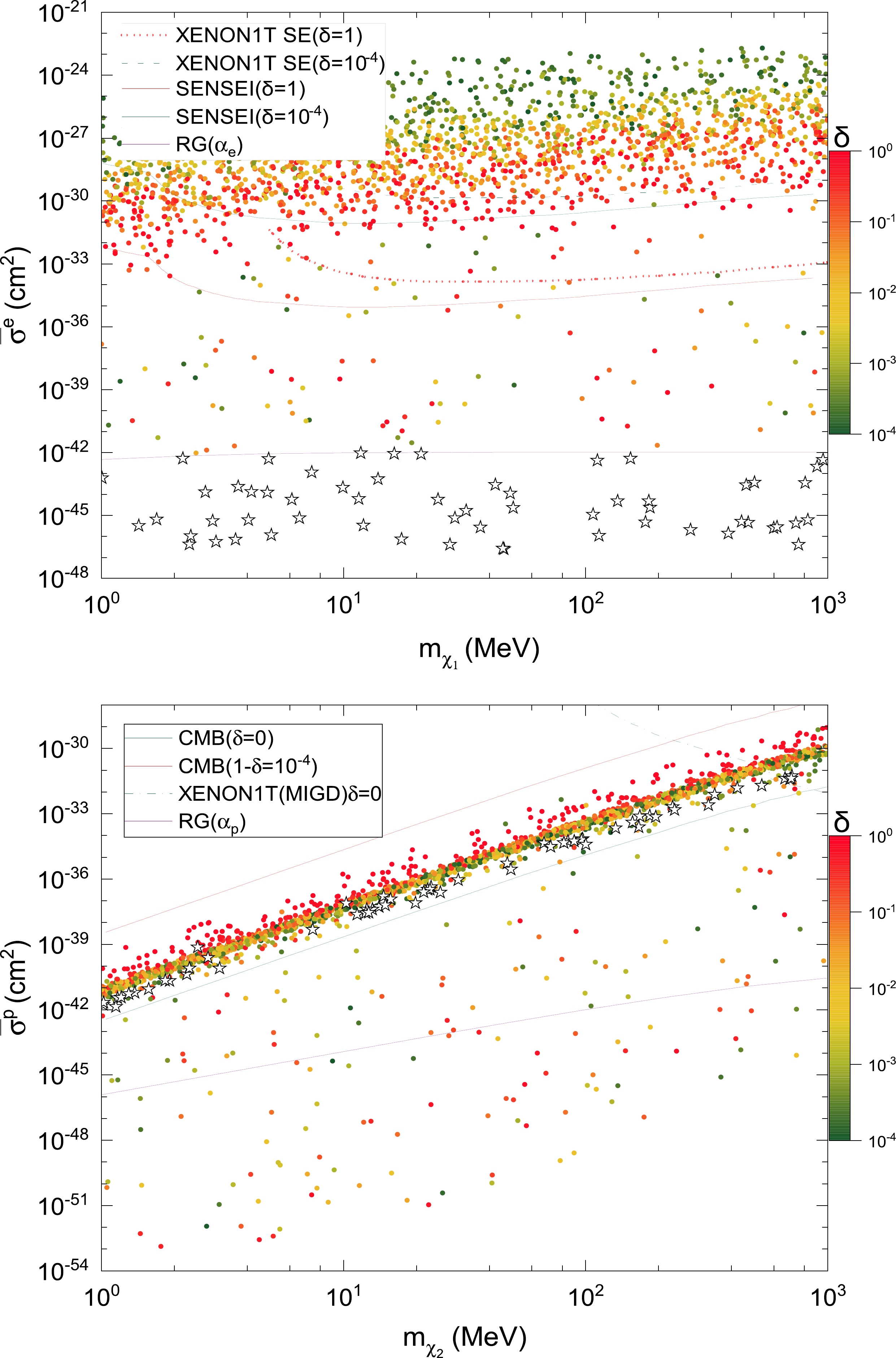
Figure 3. (color online) Samples yielding
$ -500 \leq \left<T_{21}\right> \leq -300 $ mK reported by the EDGES experiment in two-component DM with$ m_{\omega_{1}}=m_{\omega_{2}}=1 $ eV, which are projected to the plot of$ m_{\chi_{1}}-\bar{\sigma}^{e} $ ($ \mathbf{top} $ ) and$ m_{\chi_{2}}-\bar{\sigma}^{p} $ ($ \mathbf{bottom} $ ), with the dependence on the fraction parameter δ highlighted. We also present the same constraints as in Fig. 2 for comparison, with the dependences of the DM direct detection and CMB limits on δ illustrated for explicit values of$ \delta\approx \{0, 10^{-4},1\} $ .
Figure 4. (color online) Same as Fig. 3, but with
$ m_{\omega_{1}}=1 $ eV and$ m_{\omega_{2}}=10^{2} $ eV.Similar to the previous one-component case, the exclusion is robust. This result applies to simplified two-component freeze-in DM with the two light force carriers as two scalars, such as two ALPs, with spin-dependent couplings to SM quarks and leptons, among others.
-
The brightness temperature of the hydrogen 21-cm line reported by the EDGES experiment implies that the temperature of baryon gas is lower than the prediction of ΛCDM. To cool the baryon gas after kinetic decoupling, it is natural to consider the DM-baryon interaction. DM-baryon interactions with magnitudes of the scattering cross sections below current DM direct detection thresholds barely accommodate the observed signal, unless they are velocity-dependent, such as in the Coulomb-like interaction. Previous studies have shown that this type of interaction is still inadequate in simple freeze-in DM models. In this study, we perform a model-independent analysis on the parameter space in one-component and two-component freeze-in DM with the light force carrier(s) other than photons. To achieve this, we provide necessary background materials such as the conversion of the two different cross sections used by relevant experiments and the Boltzmann equations that govern the temperature evolution of both DM and baryon fluid. We show that both cases are robustly excluded by stringent stellar cooling bounds, if not by DM direct detection, etc., in the sub-GeV DM mass range. The exclusion of the one-component case applies to the freeze-in DM model with the light force carrier as gauged
$ B-L $ ,$ L_{e}-L_{\mu} $ ,$ L_{e}-L_{\tau} $ , dark photons, or ALPs, whereas the exclusion of the two-component case applies to the freeze-in DM model with the two light force carriers as two scalars, such as two ALPs, with spin-dependent couplings to SM quarks and leptons. These new results, together with earlier findings in literature, nearly close the barrier of (simplified) freeze-in DM with the Coulomb-like interaction with baryon gas as a solution to the EDGES 21-cm signal.
Freeze-in dark matter in EDGES 21-cm signal
- Received Date: 2023-02-27
- Available Online: 2023-09-15
Abstract: The first measurement of the temperature of the hydrogen 21-cm signal reported by EDGES strongly favors the Coulomb-like interaction between freeze-in dark matter and baryon fluid. We investigate such dark matter in both the one- and two-component context with the light force carrier(s) essential for the Coulomb-like interaction being other than photons. Using a conversion of cross sections used by relevant experiments and Boltzmann equations to encode the effects of the dark matter-baryon interaction, we show that both cases are robustly excluded by the stringent stellar cooling bounds in the sub-GeV dark matter mass range. The exclusion of the one-component case applies to simplified freeze-in dark matter with the light force carrier as dark photons, gauged


 DownLoad: