


 Abstract
 HTML
HTML Reference
 Related
 PDF
PDF


-
The anomalous magnetic moment of a muon, denoted as
$ a_\mu=(g_\mu-2)/2 $ , plays a crucial role in the precision tests of the Standard Model (SM) [1, 2]. The long-standing discrepancy between the SM prediction of$ a_\mu $ and its experimental measurement has recently been updated to 4.2 standard deviations [3, 4], and it has sparked numerous theoretical investigations. The SM uncertainty on$ a_\mu $ is dominated by hadronic vacuum polarization (HVP), with the largest contribution originating from the$ \pi\pi $ intermediate states, accounting for over 70% of the HVP contribution. Theoretically, the two-pion low-energy contribution to$ a_\mu $ is expressed as an integral over the modulus squared of the pion electromagnetic form factor, which can be extracted from$ e^+ e^- $ -annihilation experiments. In principle, the two-pion contribution to$ a_\mu $ can be evaluated accurately as long as the experimental data of$ e^+ e^- \to \pi^+\pi^- $ are available everywhere at the required level of precision. Although it is known that a tension exists between the two most precise measurements by BaBar and KLOE Collaborations, the BaBar data lie systematically above the KLOE results in the dominant ρ region. Consequently, considerable efforts have been dedicated to finely describing the pion electromagnetic form factor [5−11]. In the dominant ρ region of the$ e^+ e^- \to \pi^+\pi^- $ process, the isospin-breaking effect due to$ \rho-\omega $ mixing, which becomes enhanced by the small mass difference between ρ and ω mesons, plays a significant role and should be considered appropriately.Usually, the momentum dependence of
$ \rho-\omega $ mixing amplitude is neglected, and a constant mixing amplitude is used to describe$ e^+ e^- \to \pi^+\pi^- $ data due to the narrowness of the ω resonance. The first study on the momentum dependence of$ \rho-\omega $ mixing amplitude was conducted by Ref. [12]. Based on a quark loop mechanism of$ \rho-\omega $ mixing, it was determined that the mixing amplitude significantly depends on momentum. Subsequently, the investigation of various loop mechanisms for$ \rho-\omega $ mixing was initiated in different models, such as the global color model [13], extended Nambu-Jona-Lasinio (NJL) model [14, 15], chiral constituent quark model [16, 17], and hidden local symmetry model [18−20]. In our pervious study [21], we examined$ \rho-\omega $ mixing using a model independent approach through Resonance Chiral Theory (RχT) [22]. Guided by chiral symmetry and large$ N_C $ expansion, RχT provides us a reliable theoretical framework to study the dynamics with light flavor resonances and pseudo-Goldstone mesons in the intermediate energy region [23−28], and it has been successfully applied in the calculation of$ a_\mu $ in the SM [9, 29−36]. In Ref. [21], we calculated the one-loop contributions to$ \rho-\omega $ mixing, which are at the next-to-leading order (NLO) in the$ 1/N_C $ expansion [28, 37−40]. In this study, we update the previous study [21] by incorporating the contribution arising from the kaon mass splitting in the kaon loops.Moreover, we focus on analysing the impact of the momentum dependence of
$ \rho-\omega $ mixing on describing the pion vector form factor data and its contribution to$ a_\mu $ . Specifically, we perform two types of fits (with momentum-independent or momentum-dependent$ \rho-\omega $ mixing amplitude) describing$ e^+e^-\rightarrow \pi^+\pi^- $ and and$ \tau\rightarrow \nu_{\tau}2\pi $ data in the energy region of 600–900 MeV, decay width of$ \omega \rightarrow \pi^+\pi^- $ , and compare their results. The fit results demonstrate that the momentum-independent and momentum-dependent$ \rho-\omega $ mixing schemes can effectively describe the data, while the momentum-dependent scheme exhibits higher self-consistency due to the reasonable imaginary part of the extracted mixing matrix element$ \Pi_{\rho\omega} $ . Regarding the contribution to the anomalous magnetic moment of a muon,$ a_\mu^{\text{HVP,LO}}[\pi^+\pi^-] $ , which is evaluated between 0.6 GeV and 0.9 GeV, the results obtained from fits considering the momentum-dependent$ \rho-\omega $ mixing amplitude are in good agreement with those from fits that do not include the momentum dependence of$ \rho-\omega $ mixing, within the margin of errors.This paper is organized as follows. In Sec. II, we introduce the description of
$ \rho-\omega $ mixing and elaborate on the calculation of$ \rho-\omega $ mixing amplitude up to the next-to-leading order in the$ 1/N_C $ expansion. In Sec. III, the fit results are shown and related phenomenologies are discussed. A summary is provided in Sec. IV. -
In the isospin basis
$ |I,I_3\rangle $ , we define the pure isospin states$ |\rho_I\rangle\equiv |1,0\rangle $ and$ |\omega_I\rangle\equiv |0,0\rangle $ . The mixing between the isospin states of$ |\rho_I\rangle $ and$ |\omega_I\rangle $ can be implemented by considering the self-energy matrix$ \begin{eqnarray} \Pi_{\mu\nu}=T_{\mu\nu}\left( \begin{array}{cc} \Pi_{\rho\rho}(s) & \Pi_{\rho\omega}(s) \\ \Pi_{\rho\omega}(s) & \Pi_{\omega\omega}(s) \\ \end{array} \right)\,, \end{eqnarray} $

(1) with
$ T_{\mu\nu}\equiv g_{\mu\nu}- \dfrac{p^\mu p^\nu}{p^2} $ and$ s\equiv p^2 $ . The none-zero off-diagonal matrix element$ \Pi_{\rho\omega}(s) $ contains information on$ \rho-\omega $ mixing. The mixing between the physical states of$ \rho^0 $ and ω, is obtainable by introducing the following relation$ \begin{eqnarray} \left( \begin{array}{c} \rho^0 \\ \omega \end{array} \right) =C \left( \begin{array}{c} \rho_I \\ \omega_I \end{array} \right)\,,\qquad C= \left(\begin{array}{cc} 1 & -\epsilon_1 \\ \epsilon_2 & 1 \end{array} \right), \end{eqnarray} $

(2) where
$ \epsilon_1 $ and$ \epsilon_2 $ denote the mixing parameters. The matrix of dressed propagators corresponding to physical states is diagonal [41],$ \begin{eqnarray} \left( \begin{array}{cc} 1/s_{\rho} & 0 \\ 0 & 1/s_{\omega} \end{array} \right)=C \left( \begin{array}{cc} 1/s_{\rho} & \Pi_{\rho\omega}/s_{\rho}s_{\omega} \\ \Pi_{\rho\omega}/s_{\rho}s_{\omega} & 1/s_{\omega} \end{array} \right) C^{-1}, \end{eqnarray} $

(3) where abbreviations
$ s_\rho $ and$ s_\omega $ are defined by the following:$ \begin{aligned}[b] s_\rho&\equiv s-\Pi_{\rho\rho}(s)-m_\rho^2, \\ s_\omega&\equiv s-\Pi_{\omega\omega}(s)-m_\omega^2. \end{aligned} $

(4) The information of
$ \rho-\omega $ mixing is encoded in the off-diagonal element of the self-energy matrix, decomposed as follows:$ \begin{eqnarray} \Pi_{\rho\omega}(s)=\Delta_{ud}\,S_{\rho\omega}(s)+4\pi\alpha\,E_{\rho\omega}(s)\ , \end{eqnarray} $

(5) where
$ \Delta_{ud}=m_u-m_d $ denotes the mass difference between u and d quarks, and α denotes the fine-structure constant.$ S_{\rho\omega}(s) $ and$ E_{\rho\omega}(s) $ denote the structure functions of the strong and electromagnetic interactions, respectively. In this study, the diagrams in Fig. 1 are calculated in RχT up to NLO in$ 1/N_C $ expansion.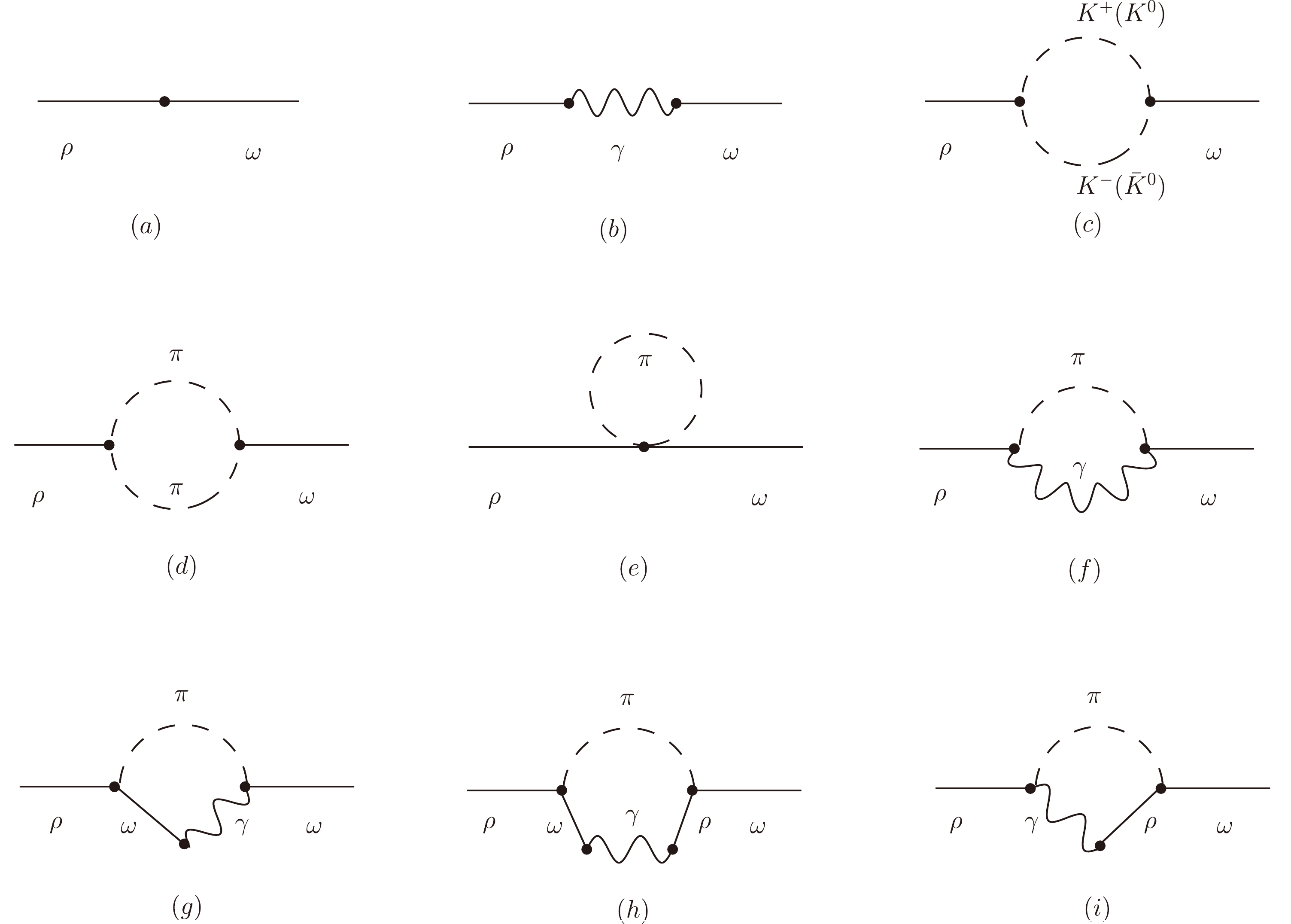
Figure 1. Feynman diagrams contributing to
$ \rho-\omega $ mixing.In RχT, the vector resonances can be described in terms of antisymmetric tensor fields with normalization:
$ \begin{eqnarray} \langle 0|V_{\mu\nu}|V,p\rangle ={\rm i} M_V^{-1}\{p_\mu\epsilon_\nu(p)-p_\nu\epsilon_\mu(p)\}, \end{eqnarray} $

(6) where
$ \epsilon_\mu $ denotes the polarization vector. Here, the vector mesons are collected in a$ 3\times3 $ matrix as follows:$ \begin{equation} V_{\mu\nu}= \left( {\begin{array}{*{3}c} \dfrac{1}{\sqrt{2}}\rho^0 +\dfrac{1}{\sqrt{2}}\omega & {\rho^+ } & {K^{\ast+} } \\ {\rho^- } & -\dfrac{1}{\sqrt{2}}\rho ^0 +\dfrac{1}{\sqrt{2}}\omega & {K^{\ast0} } \\ { K^{\ast-}} & {\overline{K}^{\ast0} } & -\phi \\ \end{array}} \right)_{\mu\nu}\,. \end{equation} $

(7) The effective Lagrangian for the leading order strong isospin-breaking effect, corresponding to the tree-level contribution diagram (a) in Fig. 1, is as follows [42, 43]:
$ \begin{eqnarray} \mathcal{L}_2^{\rho\omega}=\lambda_6^{VV}\langle V_{\mu\nu}V^{\mu\nu}\chi_+\rangle \,, \end{eqnarray} $

(8) with
$ \chi_+=u^{+}\chi u^{+}+ u\chi^{+}u $ and$\chi=2B_0(s+{\rm i}p)$ . The pseudo-Goldstone bosons originating from the spontaneous breaking of chiral symmetry can be filled nonlinearly into:$ \begin{aligned}[b] u_\mu =& {\rm i} \left( u^\dagger\partial_\mu u\, -\, u \partial_\mu u^\dagger\right) \,, \\ u =& \exp \Bigg( \frac{{\rm i}\Phi}{\sqrt{2}F} \Bigg)\,, \end{aligned} $

(9) with the Goldstone fields
$ \begin{align} \Phi &= \begin{pmatrix} {\dfrac{1}{\sqrt{2}}\pi ^0 +\dfrac{1}{\sqrt{6}}\eta } & {\pi^+ } & {K^+ } \\ {\pi^- } & {-\dfrac{1}{\sqrt{2}}\pi ^0 +\dfrac{1}{\sqrt{6}}\eta} & {K^0 } \\ { K^-} & {\bar{K}^0 } & {-\dfrac{2}{\sqrt{6}}\eta} \\ \end{pmatrix} . \end{align} $

(10) where F denotes the pion decay constant. Considering the mass relations of the vector mesons at
$ O(p^2) $ in terms of the quark counting rule, the value of the coupling constant is determined as follows:$ \lambda_6^{VV}=1/8 $ [42, 43]. Thus, the tree-level strong contribution can be expressed as follows:$ \begin{eqnarray} S_{\rho\omega}^{(a)}=2\,M_V \ . \end{eqnarray} $

(11) The Lagrangian describing the interactions between
$ V_{\mu\nu} $ and electromagnetic fields or Goldstone bosons are as follows:$ \begin{eqnarray} \mathcal{L}_{2}(V)&=&\frac{F_V}{2\sqrt{2}}\langle V_{\mu\nu}f_+^{\mu\nu}\rangle+\frac{{\rm i}G_V}{\sqrt{2}}\langle V_{\mu\nu}u^\mu u^\nu\rangle\ , \end{eqnarray} $

(12) with the relevant building blocks defined as follows:
$ \begin{aligned}[b] u_\mu =&{\rm i}[u^+(\partial _\mu \ -{\rm i}r_\mu)u-u(\partial _\mu -{\rm i}l_\mu)u^+]\,, \\ f_{\pm}^{\mu\nu}=&uF_L^{\mu\nu}u^+\pm u^+F_R^{\mu\nu}u \,. \end{aligned} $

(13) Here,
$ F_{L,R}^{\mu\nu} $ denote field strength tensors composed of the left and right external sources$ l_\mu $ and$ r_\mu $ , and$ F_V $ and$ G_V $ denote real resonance couplings constants. The tree-level electromagnetic contribution from diagram (b) in Fig. 1 can be calculated using the Lagrangian in Eq. (12):$ \begin{eqnarray} E_{\rho\omega}^{(b)}=\frac{ F_\rho F_\omega}{3}\,. \end{eqnarray} $

(14) The physical decay constants
$ F_\rho $ and$ F_\omega $ have been employed in the amplitude, and are differentiated by means of isospin breaking.The loop contributions of diagrams (d)–(i) in Fig. 1 have been extensively discussed in our previous study [21]. However, a noteworthy distinction in our current study is the inclusion of the contribution from diagram (c), which arises from the kaon mass splitting within the kaon loops. To ensure comprehensiveness, we present the expressions for the loop contributions in the Appendix A. Furthermore, it should be noted that the ultimate expression for the renormalized mixing amplitude
$ {\Pi}_{\rho\omega}(p^2) $ is presented in Eq. (A23). -
The mass and width of the ρ meson are conventionally determined by fitting to the experimental data of
$ e^+e^-\rightarrow \pi^+\pi^- $ and$ \tau\rightarrow \nu_{\tau}2\pi $ [44], where various mechanisms are used to describe$ \rho-\omega $ mixing effect. To prevent interference due to their$ \rho-\omega $ mixing mechanisms, we treat mass$ M_\rho $ and relevant couplings$ G_\rho $ and$ F_\rho $ as free parameters in our fit. Regarding its width, the energy-dependent form is constructed in a similar manner as introduced in [45]:$ \begin{eqnarray} \Gamma_{\rho}(s)=\frac{sM_\rho}{96\pi F^2}\left[\sigma_\pi^3\theta(s-4m_\pi^2)+\frac{1}{2}\sigma_K^3\theta(s-4m_K^2)\right]\,, \end{eqnarray} $

(15) where
$ \sigma_{P} \equiv \sqrt{1-4m_{P}^{2}/s} $ and$ \theta(s) $ is the step function.With respect to the ω mass, it has been indicated in Refs. [5, 7] that the result determined from
$ e^+e^- \rightarrow \pi^+\pi^- $ is inconsistent with that from particle data group (PDG) [44], primarily determined by experiments involving$ e^+e^- \rightarrow 3\pi $ and$ e^+e^- \rightarrow \pi^0\gamma $ . Therefore, we treated the ω mass and width as free parameters and estimated them by fitting in our programme. The physical coupling$ F_\omega $ can be determined from the decay width of$ \omega\rightarrow e^+e^- $ . Using the Lagrangian formula in Eq. (12), the decay width can be derived as follows:$ \begin{eqnarray} \Gamma_{\omega}^{e^+e^-}=\frac{4\alpha^2\pi F_\omega^2(2m_e^2+M_\omega^2)\sqrt{M_\omega^2-4m_e^2}}{27 M_\omega^4}\,, \end{eqnarray} $

(16) Hence, the expression for
$ F_\omega $ can be obtained. Based on the decay widths provided above,$ s_\rho $ and$ s_\omega $ in Eq. (4) can be rewritten as$ \begin{aligned}[b] s_\rho\simeq& s-M_{\rho}^2+{\rm i}M_{\rho}\Gamma_{\rho}(s) \ ,\\ s_\omega\simeq& s-M_{\omega}^2+{\rm i}M_{\omega}\Gamma_{\omega}\ . \end{aligned} $

(17) The pion form-factor in
$ \tau\rightarrow \nu_{\tau}2\pi $ decay, irrelevant to$ \rho-\omega $ mixing effect, were thoroughly examined in Refs. [36, 46−48]:$ \begin{aligned}[b] F_\pi^\tau(s)=&\Bigg(1-\frac{G_\rho F_\rho s}{F^2}\frac{1}{s_{\rho}}\Bigg)\\& \times \exp\left\{\frac{-s}{96\pi^{2}F^{2}}\left({\rm Re}\left[A[m_{\pi},M_{\rho},s]+\frac{1}{2}A[m_{K},M_{\rho},s]\right]\right)\right\}\,. \end{aligned} $

(18) Furthemorme, function
$ \begin{eqnarray} A\left(m_{P},\mu,s\right) = \ln\left(m_{P}^{2}/\mu^{2}\right)+\frac{8m_{P}^{2}}{s}-\frac{5}{3}+\sigma_{P}^{3}\ln\left(\frac{\sigma_{P}+1}{\sigma_{P}-1}\right) \, . \end{eqnarray} $

(19) To incorporate isospin-breaking effects, one approach involves multiplying
$ |F_\pi^\tau(s)|^2 $ by factor$ S_{\rm EW}G_{\rm EM}(s) $ , where$ S_{\rm EW}=1.0233 $ corresponds to the short distance correction [49]. Additionally,$ G_{\rm EM}(s) $ accounts for the long-distance radiative correction, as described in [50]. Specifically, in our fit of$ \tau\rightarrow \nu_{\tau}2\pi $ decay data, we perform the following substitution.$ \begin{eqnarray} |F_\pi^\tau(s)|^2\Rightarrow S_{\rm EW}G_{\rm EM}(s)|F_\pi^\tau(s)|^2. \end{eqnarray} $

(20) The pion form-factor in
$ e^+e^- $ annihilation is as follows:$ \begin{aligned}[b] F_\pi^{ee}(s)=&\Bigg[1-\frac{G_\rho F_\rho s}{F^2}\frac{1}{s_{\rho}}-\frac{G_\rho F_\omega s}{3F^2}\frac{1}{s_\omega}\Pi_{\rho\omega}\frac{1}{s_{\rho}} \\&-\frac{4\sqrt{2}aB_0F_\omega(m_u-m_d)s}{3F^2}\frac{1}{s_\omega}\Bigg] \\ & \times \exp\Bigg\{\frac{-s}{96\pi^{2}F^{2}}\Bigg({\rm Re}\Bigg[A[m_{\pi},M_{\rho},s]\\&+\frac{1}{2}A[m_{K},M_{\rho},s]\Bigg]\Bigg)\Bigg\}\,. \end{aligned} $

(21) As defined in Appendix A.2, parameter a is associated with the combined coupling constant of the direct
$ \omega\pi\pi $ interaction. In the first bracket of Eq. (21), the second term corresponds to the contribution from$ \rho\pi\pi $ coupling, third term represents the contribution of$ \rho-\omega $ mixing, and fourth term corresponds to contribution from the direct isospin-breaking coupling of ω to the pion pair.The leading order contribution of
$ \pi\pi(\gamma) $ intermediate state to the anomalous magnetic moment of the muon is as follows [51]:$ \begin{equation} a_{\mu}^{\pi\pi(\gamma),\text{LO} }=\left(\frac{\alpha m_{\mu}}{3\pi}\right)^{2}\int_{4 m_\pi^2}^{\infty}\mathrm{d}s\frac{\hat{K}(s)}{s^{2}}R_{\pi\pi(\gamma)}(s)\text{,} \end{equation} $

(22) where
$ \begin{eqnarray} R_{\pi\pi(\gamma)}(s)=\frac{3s}{4\pi\alpha^{2}} \, \sigma^{(0)}\left(e^+e^-\rightarrow \pi\pi(\gamma)\right)\ , \end{eqnarray} $

(23) and the kernel function is defined as follows:
$ \begin{aligned}[b] \hat{K}(s)=&\frac{3s}{m_{\mu}^{2}}\Bigg[\frac{\left(1+x^{2}\right)(1+x)^{2}}{x^{2}}\left(\ln(1+x)-x+\frac{x^{2}}{2}\right)\\&+\frac{x^{2}}{2}\left(2-x^{2}\right)+\frac{1+x}{1-x}x^{2}\ln x\Bigg]\text{ ,} \end{aligned} $

(24) with
$ \begin{eqnarray} x=\frac{1-\beta_{\mu}(s)}{1+\beta_{\mu}(s)}, & \quad & \qquad \beta_{\mu}(s)=\sqrt{1-\frac{4m_{\mu}^{2}}{s}}\ . \end{eqnarray} $

(25) It should be noted that in the formula for
$ a_{\mu}^{\pi\pi(\gamma),\text{LO} } $ in Eq. (22), the integration is performed from 4$ m_\pi^2 $ to$ \infty $ . In this study, we focus on the momentum dependence of$ \rho-\omega $ mixing. Therefore, we only describe the pion vector form factor up to 900 MeV. To extend the study by considering higher energies, we must consider the effects of excited resonances, including$ \rho^\prime(1450) $ and$ \rho^{\prime\prime}(1700) $ . However, these effects are beyond the scope of this study. It is interesting to note that the$ 1/s^2 $ enhancement factor in Eq. (22) provides higher weight to the lowest lying resonance$ \rho(770) $ that couples strongly to$ \pi^+\pi^- $ .The bare cross section, including final-state radiation, takes the following form [5, 52−54]:
$ \begin{aligned}[b]& \sigma^{(0)}(e^+e^-\to\gamma^*\to\pi^+\pi^-(\gamma))\\ =& \Big[ 1 + \frac{\alpha}{\pi} \eta(s) \Big] \frac{\pi \big|\alpha(s)\big|^2}{3s} \sigma_\pi^3(s) \big| F_\pi^{ee}(s) \big|^2 \frac{s+2m_e^2}{s \sigma_e(s)}, \end{aligned} $

(26) where
$ \begin{aligned}[b] \eta(s) =& \frac{3(1+\sigma_\pi^2(s))}{2\sigma_\pi^2(s)} - 4 \log\sigma_\pi(s) + 6 \log \frac{1+\sigma_\pi(s)}{2} + \frac{1+\sigma_\pi^2(s)}{\sigma_\pi(s)} F(\sigma_\pi(s)) \\& - \frac{(1-\sigma_\pi(s))\big(3+3\sigma_\pi(s)-7\sigma_\pi^2(s)+5\sigma_\pi^3(s)\big)}{4\sigma_\pi^3(s)} \log\frac{1+\sigma_\pi(s)}{1-\sigma_\pi(s)}, \\ F(x) =& -4 \mathrm{Li}_2(x)+4 \mathrm{Li}_2(-x)+2\log x \log\frac{1+x}{1-x} + 3 \mathrm{Li}_2\Big(\frac{1+x}{2} \Big) - 3 \mathrm{Li}_2\Big(\frac{1-x}{2} \Big) + \frac{\pi^2}{2}, \\ \mathrm{Li}_2(x) =& - \int_0^x {\rm d} t \frac{\log(1-t)}{t}. \end{aligned} $ 
(27) The experimental data considered in this study are the pion form factor
$ F_\pi^{ee}(s) $ of the$ e^+e^-\rightarrow \pi^+\pi^- $ process measured by the OLYA [55], CMD [56], BaBar [57], BESIII [58], KLOE [59], CLEO [60], and SND [61] Collaborations, the form factor$ F_\pi^\tau(s) $ of$ \tau\rightarrow \nu_{\tau}2\pi $ decay measured by the ALEPH [62] and CLEO [63] Collaborations, and the decay width of$ \omega \rightarrow \pi^+\pi^- $ [44]. It should be noted that in the experimentally published form factor data$ F_\pi^{ee}(s) $ , the vacuum polarization effects have been excluded through the subtraction of the hadronic running of$ \alpha(s) $ . Thus, in our fitting of the form factor data$ F_\pi^{ee}(s) $ , the one-photon-reducible Fig. 1(b) should not be considered. Given that we focus on the analysis of the$ \rho-\omega $ mixing effect, we only take into account the form factors$ F_\pi^{ee}(s) $ and$ F_\pi^{\tau}(s) $ data in the energy region of 600–900 MeV. It should be noted that for the pion form factor$ F_\pi^{ee}(s) $ , a tension is observed between the two most precise measurements from BaBar and KLOE in theρ peak region. However, other measurements align with theirs within the stated uncertainties. This highlights the impact of momentum dependence of $ \rho-\omega $ mixing, and to avoid the tension between BaBar and KLOE data, we conduct four separate fits. Specifically, in Fits Ia and Ib, we fit all data sets excluding BaBar with momentum-independent$ \Pi_{\rho\omega} $ and momentum-dependent$ \Pi_{\rho\omega} $ , respectively. In Fits IIa and IIb, we fit all data sets excluding KLOE with momentum-independent$ \Pi_{\rho\omega} $ and momentum-dependent$ \Pi_{\rho\omega} $ , respectively. Fits Ia and IIa involve eight free parameters:$ M_\rho $ ,$ G_\rho $ ,$ F_\rho $ ,$ M_\omega $ ,$ \Gamma_\omega $ , a, and the real and imaginary part of constant$ \Pi_{\rho\omega} $ . There are nine free parameters in Fits Ib and IIb:$ M_\rho $ ,$ G_\rho $ ,$ F_\rho $ ,$ M_\omega $ ,$ \Gamma_\omega $ , a,$ X_W^r $ ,$ X_Z^r $ , and$ X_R^r $ . As defined in the Appendix A,$ X_W^r $ ,$ X_Z^r $ , and$ X_R^r $ are the corresponding parameters for the counterterms.In Fig. 2, the fitted results of the fits using momentum-independent
$ \Pi_{\rho\omega} $ (Fits Ia and IIa) and momentum-dependent$ \Pi_{\rho\omega} $ (Fits Ib and IIb) are shown as red dotted lines and black solid lines, respectively. The fitted parameters as well as$ \chi^2/\text{d.o.f.} $ are listed in Table 1. It is intriguing to compare the results obtained from fits utilising momentum-independent$ \Pi_{\rho\omega} $ and momentum-dependent$ \Pi_{\rho\omega} $ for the same datasets. Specifically, we compare Fit Ia and Ib and Fit IIa and IIb. When examining pion form factors$ |F_\pi^{ee}(s)|^2 $ and$ |F_\pi^{\tau}(s)|^2 $ , we observe that the differences between the theoretical predictions of the fits using momentum-independent$ \Pi_{\rho\omega} $ and the corresponding ones using momentum-dependent$ \Pi_{\rho\omega} $ are low. Furthermore, it should be noted that for the pion form factor$ |F_\pi^{ee}(s)|^2 $ in Fits Ia and Ib, the theoretical predictions are much higher than the KLOE data at ρ peak, and these deviations contribute significantly to their value of$ \chi^2 $ . Thus, we conclude that the momentum-independent$ \Pi_{\rho\omega} $ and momentum-dependent$ \Pi_{\rho\omega} $ can describe the data well, and the discordances among different collaborations contribute significantly to$ \chi^2 $ values in the fits.
Figure 2. (color online) Fit results of the pion form factor in the
$ e^+e^- \rightarrow \pi^+\pi^- $ process (left panel) and$ \tau\rightarrow \nu_\tau 2\pi $ process (right panel) in the energy region of 600–900 MeV. The data of$ e^+e^- $ annihilation are considered from OLYA (Gray) [55], CMD (Yellow) [56], BaBar (Blue) [57], BESIII (Green) [58], KLOE (Cyan) [59], CLEO (Magenta) [60], and SND (Orange) [61] Collaborations. The τ decay data are taken from the ALEPH (Orange) [62], and CLEO (Green) [63] collaborations. Fits Ia and Ib fit all data sets excluding BaBar (top), and Fits IIa and IIb fit all data sets excluding KLOE (bottom). Fits Ia and IIa use momentum-independent$ \Pi_{\rho\omega} $ and are denoted by the red dashed lines. Fits Ib and IIb use momentum-dependent$ \Pi_{\rho\omega} $ and are denoted by the black solid lines. The vertical lines lie at$ M_\rho $ ,$ M_\omega $ , and$ 2M_\omega-M_\rho $ (from left to right).Fit Ia Fit Ib Fit IIa Fit IIb $ M_\rho $ /MeV

$ 775.35 \pm 0.10 $ 

$ 775.68 \pm 0.12 $ 

$ 775.45\pm0.10 $ 

$ 775.55\pm0.11 $ 

$ G_\rho $ /MeV

$ 55.25 \pm 0.09 $ 

$ 55.74 \pm 0.08 $ 

$ 54.21\pm0.09 $ 

$ 55.03\pm0.07 $ 

$ F_\rho $ /MeV

$ 152.65\pm 0.29 $ 

$ 151.40\pm 0.21 $ 

$ 155.65\pm0.23 $ 

$ 153.38\pm0.31 $ 

$ M_\omega $ /MeV

$ 782.59 \pm 0.13 $ 

$ 782.68 \pm 0.12 $ 

$ 782.39\pm0.11 $ 

$ 782.45\pm0.11 $ 

$ \Gamma_\omega $ /MeV

$ 8.97 \pm 0.27 $ 

$ 9.03 \pm 0.26 $ 

$ 8.04\pm0.16 $ 

$ 8.16\pm0.17 $ 

$a /\text{GeV}^{-1}$ 

$ -0.0020\pm 0.0150 $ 

$ -0.0054\pm 0.0010 $ 

$ -0.1066\pm0.0152 $ 

$ -0.0067\pm0.0009 $ 

$\text{Re}(\Pi_{\rho\omega}) /\text{MeV}^2$ 

$ -3372 \pm 112 $ 

− $ -3799 \pm 85 $ 

− $\text{Im}(\Pi_{\rho\omega}) /\text{MeV}^2$ 

$ 296\pm 669 $ 

− $ -4544 \pm 704 $ 

− $X_W^r /\text{GeV}^{-6}$ 

− $ -0.141\pm 0.013 $ 

− $ -0.177\pm0.008 $ 

$X_Z^r /\text{GeV}^{-4}$ 

− $ 0.195\pm 0.016 $ 

− $ 0.303\pm0.007 $ 

$X_R^r /\text{GeV}^{-2}$ 

− $ -0.081\pm 0.006 $ 

− $ -0.133\pm0.003 $ 

$ {\chi^2}/{\rm d.o.f.} $ 

$ \dfrac{410.7}{(238-8)}=1.79 $ 

$ \dfrac{405.8}{(238-9)}=1.77 $ 

$ \dfrac{392.2}{(341-8)}=1.18 $ 

$ \dfrac{394.6}{(341-9)}=1.19 $ 

$ a_\mu^{\pi\pi}|_{[0.6,0.9] \text{GeV}} [\times 10^{10}] $ 

$ 367.72\pm 1.07 $ 

$ 367.80\pm 2.92 $ 

$ 375.41\pm 1.03 $ 

$ 375.29\pm2.21 $ 

Table 1. Fit results of the parameters. Fits Ia and Ib fit all data sets excluding BaBar, and Fits IIa and IIb fit all data sets excluding KLOE. Fits Ia and IIa use momentum-independent
$ \Pi_{\rho\omega} $ , while Fits Ib and IIb use momentum-dependent$ \Pi_{\rho\omega} $ .In the last line of Table 1, we provide the results of
$ a_\mu^{\text{HVP,LO}}[\pi^+\pi^-] $ , evaluated between 0.6 GeV and 0.9 GeV. The differences between the results using the momentum-independent$ \Pi_{\rho\omega} $ and the results using the momentum-dependent$ \Pi_{\rho\omega} $ for the same datasets, namely the differences between Fits Ia and Ib and Fits IIa and IIb, respectively, are negligible.In Fig. 3, we plot the real and imaginary parts of the mixing amplitudes
$ \Pi_{\rho\omega}(s) $ in Fits Ib and IIb. It is determined that the real part is dominant within$ \rho-\omega $ mixing region. The real part in Fit IIb demonstrates a significant momentum dependence, whereas the real part in Fit Ib displays a smooth momentum dependence. Additionally, it should be noted that the real parts of the two fits nearly reach the same point at$ s^{1/2}=M_\omega $ . In comparison to the real part, the imaginary part is rather small. At$ s=M_\omega^2 $ , in Fit Ib the mixing amplitude$\Pi_{\rho\omega}(M_\omega^2)=(-3405.0+62.1{\rm i})$ MeV$ ^2 $ , and in Fit IIb$\Pi_{\rho\omega}(M_\omega^2)=(-3316.3+113.7{\rm i})$ MeV$ ^2 $ . The minimal magnitude of the imaginary part aligns with the findings presented in Refs. [64, 65]. However, therein the effect of direct$ \omega_I \rightarrow \pi^+\pi^- $ was not considered. It is worth mentioning that larger imaginary part is obtained in [13, 17] by using global color model and a chiral constituent quark model, respectively. By utilising our fitted parameter results, we proceed to calculate the ratio of the two-pion couplings associated with the isospin-pure ω and ρ.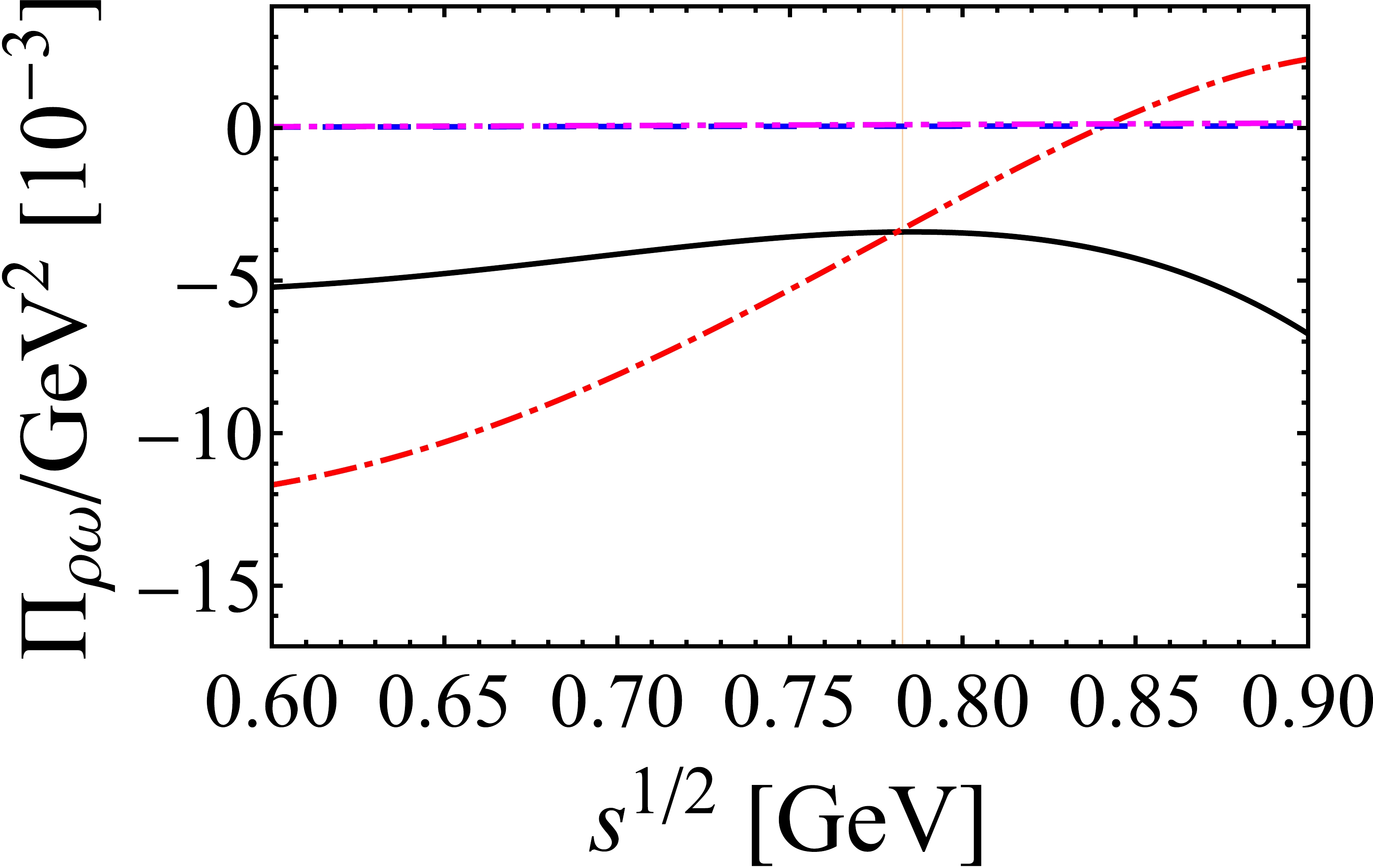
Figure 3. (color online) Momentum dependence of the mixing amplitudes
$ \Pi_{\rho\omega}(s) $ . The black solid and red dot-dashed lines correspond to the real part of$ \Pi_{\rho\omega}(s) $ in Fits Ib and IIb, respectively. The blue dashed and magenta dash-dot-dotted lines correspond to the imaginary part of$ \Pi_{\rho\omega}(s) $ in Fits Ib and IIb, respectively. The vertical line lies at$ M_\omega $ .$ \begin{eqnarray} G=\frac{g_{\omega_I\pi\pi}}{g_{\rho_I\pi\pi}}=\frac{4\sqrt{2}a B_0(m_u-m_d)}{G_\rho}. \end{eqnarray} $

(28) The results are
$ G=(2.1\pm1.1)\times 10^{-3} $ in Fit Ib, and$ G=(2.6\pm1.2)\times 10^{-3} $ in Fit IIb. It should be noted that the value of G is expected to be of the order$ \alpha=1/137 $ in Ref. [65]. The central values of our results of G are in good agreement with the expectation in Ref. [65], while they are lower than other two estimations, namely$ G=(5.0\pm1.7_{\text{model}}\pm 1.0_{\text{data}})\times 10^{-2} $ in [66] and$ G=(3.47\pm 0.64)\times 10^{-2} $ in [67]. As listed in Table 1, the differences in$ {\chi^2}/{\rm d.o.f.} $ between the momentum-dependent fits and momentum-independent fits for the same data sets are minimal. The$ \chi^2 $ of Fit IIa is slightly lower than the$ \chi^2 $ of Fit IIb. However, Fit IIa contains one less fitting parameter than Fit IIb. It can be observed that the magnitude of the imaginary part of$ \Pi_{\rho\omega} $ in Fit IIa is significantly greater than those in other three fits. In our framework, the imaginary part of$ \Pi_{\rho\omega} $ arises from$\pi^{0}\gamma$ and$ \pi\pi $ real intermediate states. By considering the decay widths of$ \omega \rightarrow \pi^0\gamma $ and$ \rho \rightarrow \pi^0\gamma $ , the imaginary part of$ \Pi_{\rho\omega} $ , contributed from$ \pi^0\gamma $ intermediate state, can be estimated to be approximately −150 MeV2 [7, 65]. If the estimated ratio of the two-pion couplings of the isospin-pure ω and ρ are used:$ G \sim \alpha=1/137 $ [65], then the$ \pi\pi $ intermediate state contribution to the imaginary part of$ \Pi_{\rho\omega} $ can be obtained in the order of several hundred MeV2. In our momentum-dependent scheme, the imaginary part of$ \Pi_{\rho\omega} $ due to$ \pi^0\gamma $ and$ \pi\pi $ intermediate states are explicitly computed, and the numerical results of Im$ \Pi_{\rho\omega} $ in Fits Ib and IIb are of the order of one hundred MeV2, as expected. However, in the momentum-independent Fits Ia and IIa, the imaginary part of$ \Pi_{\rho\omega} $ is a free fitting parameter. As listed in Table 1, the fitted results of Im$ \Pi_{\rho\omega} $ and parameter "a" in Fit IIa are unreasonably high. The fitted results of Im$ \Pi_{\rho\omega} $ and parameter "a" in Fit Ia exhibit large error bars. Consequently, we conclude that both momentum-independent and momentum-dependent$ \rho-\omega $ mixing schemes can describe$ e^+e^- \rightarrow \pi^+\pi^- $ data well. However, the momentum-dependent$ \rho-\omega $ mixing scheme is more self-consistent, especially given the reasonable imaginary part of$ \Pi_{\rho\omega} $ , which is extracted.We wish to emphasize that the direct
$ \omega_I\rightarrow \pi^+\pi^- $ coupling is generally an unknown quantity, and it impacts$ F_\pi^{ee}(s) $ in two ways, both through the third term in the first bracket of Eq. (21), appearing as real intermediate state in the contributions to$ \Pi_{\rho\omega} $ and through the fourth term in that bracket. Conventionally, the direct$ \omega_I\rightarrow \pi^+\pi^- $ is assumed to be neutralized in$ e^+e^- \rightarrow \pi^+\pi^- $ due to the fact that ω and ρ are quasidegenerate and that 2π channel dominates the ρ decay [65]. Theoretical models that do not neglect direct$ \omega_I\rightarrow \pi^+\pi^- $ coupling may be more comprehensive, especially given the availability of high-precision data available currently. It should be noted that in Refs. [5, 7], the pion form factor has been examined in a model-independent way using dispersion theory. Specifically,$ \rho-\omega $ mixing is subsumed in one parameter$ \epsilon_\omega $ , which should contain a small imaginary part originating from the radiative intermediate states (with an estimated phase of approximately 4 degrees). Furthemrore, given that direct$ \omega_I\rightarrow \pi^+\pi^- $ coupling is not considered in Refs. [5, 7],$ \epsilon_\omega $ term is actually a combination of$ \rho-\omega $ mixing and direct$ \omega_I\rightarrow \pi^+\pi^- $ . Therefore, it cannot be directly compared to$ \Pi_{\rho\omega} $ discussed in this context. (At$ s=M_\omega^2 $ , our$ \Pi_{\rho\omega}(M_\omega^2) $ in Fits Ib and IIb contains negative phase.) Nevertheless, the ratio between the on-ω-mass-shell$ \gamma^\ast \rightarrow \omega \rightarrow \pi\pi $ transition amplitude and$ \gamma^\ast \rightarrow \rho \rightarrow \pi\pi $ transition amplitude (without$ \pi\pi $ final state interaction) should be model independent. With$ s=M_\omega^2 $ , the ratio between the second term and first term in Eq. (2.5) of [7] yields$R_{\omega\rho}=\text{Amplitude}~({\gamma^{\ast} \rightarrow \omega \rightarrow \pi\pi})/ \text{Amplitude}~ ({\gamma^\ast \rightarrow \rho \rightarrow \pi\pi})= (0.178 \;\pm \;0.003)\;\times\; {\rm e}^{{\rm i}(4.66\pm 1.13)^\circ}$ , using Re$\epsilon_\omega= (1.97\pm 0.03)\times 10^{-3}$ and$ \delta_\epsilon=(4.5\pm 1.2)^\circ $ obtained therein. It can be observed that the difference between the phase of$ R_{\rho\omega}(M_\omega^2) $ and$ \delta_\epsilon $ is minimal. In this study, the ratio between the sum of the third term and fourth terms and the sum of the first and second terms in the first bracket of Eq. (21) predicts$R_{\omega\rho} =(0.155 \pm 0.002)\times {\rm e}^{{\rm i}(5.80\pm 1.71)^\circ}$ and$R_{\omega\rho}= (0.150 \pm 0.002)\times {\rm e}^{{\rm i}(3.67\pm 1.71)^\circ}$ in Fit Ib and IIb, respectively. It can be observed that our results of$ R_{\omega\rho} $ approximately agree with that in [7].Using the central values of the fitted parameters of our best fit (Fit IIb) in Table 1, we calculate the decay width of
$ \omega \rightarrow \pi^+\pi^- $ $ \begin{aligned}[b] \\[-7pt] \Gamma_{\omega \rightarrow \pi^+\pi^-}=&\frac{1}{192\pi F^4}(M_\omega^2-4m_\pi^2)^{\frac{3}{2}} \times \Bigg(\exp\left[\frac{-M_\omega^2}{96\pi^{2}F^{2}}\left({\rm Re}\left[A[m_{\pi},M_{\rho},M_\omega^2]+\frac{1}{2}A[m_{K},M_{\rho},M_\omega^2]\right]\right)\right]\Bigg)^2 \\ & \times \Big| 8\sqrt{2}B_0(m_u-m_d)a+\frac{2G_\rho \Pi_{\rho\omega}(M_\omega^2)}{M_\omega^2-M_\rho^2-{\rm i}(M_\omega \Gamma_\omega-M_\rho \Gamma_\rho)}\Big|^2\\ =&0.013\mid (0.29)+(-0.22+3.35{\rm i})\mid^2 \,. \end{aligned} $ 
(29) Based on Eq. (29), we can determine that the first term due to direct
$ \omega_I \rightarrow \pi^+\pi^- $ is smaller than the second term due to$ \rho-\omega $ mixing by an order of magnitude. Within 1σ uncertainties, our theoretical value of the branching fraction is$ \mathscr{B}(\omega \rightarrow \pi^+\pi^-)=(1.48\pm 0.10)\times 10^{-2} $ , which is consistent with the values provided in PDG [44] and with those reported in the recent dispersive analysis [68].Regarding the mass of the ω meson, previous studies [5, 7, 57] indicated that the result extracted from
$ e^+e^- \rightarrow \pi^+\pi^- $ is substantially lower than the current PDG average [44], which primarily relies on$ e^+e^- \rightarrow 3\pi $ and$ e^+e^- \rightarrow \pi^0\gamma $ experiments. The discrepancy amounts to approximately 1 MeV, corresponding to around 5 σ considering the current precision. It has been observed that the fitted value for$ M_\omega $ and phase of$ \epsilon_\omega $ are strongly correlated [5, 7, 57]. It should be noted that direct$ \omega_I\rightarrow \pi^+\pi^- $ coupling has not been considered in [5, 7, 57]. As indicated in Table 1 above, our fitted results for the mass of ω are in good agreement with the value in PDG:$ M_\omega= 782.66 \pm 0.13 $ MeV, and this agreement remains unaffected by the inclusion or exclusion of the momentum dependence of$ \Pi_{\rho\omega} $ . Furthermore, we can observe that a strong correlation (80%) exists between parameter "a," which quantifies the direct$ \omega_I\rightarrow \pi^+\pi^- $ coupling, and the mass of ω. As mentioned earlier, the direct$ \omega_I\rightarrow \pi^+\pi^- $ coupling influences the imaginary part and real part of the amplitude, and thereby, affects the phase of$ R_{\rho\omega}(M_\omega^2) $ . It should be noted that the phase of$ R_{\rho\omega}(M_\omega^2) $ approximately agrees with the phase of$ \epsilon_\omega $ . Thus, our observations align with with those in Refs. [5, 7, 57]. Hence, a strong correlation exists between the mass of the omega meson and phase of$ \epsilon_\omega $ . Our findings suggest that the inclusion of direct$ \omega_I\rightarrow \pi^+\pi^- $ coupling is likely crucial in the analysis aimed at extracting the ω mass from the$ e^+e^- \rightarrow \pi^+\pi^- $ process. -
We utilized the resonance chiral theory to examine
$ \rho-\omega $ mixing. Specifically, we analyzed the impact of the momentum dependence of$ \rho-\omega $ mixing on describing the pion vector form factor in the$ e^+e^-\rightarrow \pi^+\pi^- $ process and its contribution to the anomalous magnetic moment of muon$ a_\mu $ . The incorporation of momentum dependence arises from the calculation of loop contributions, which corresponds to the next-to-leading orders in$ 1/N_C $ expansion. Based on fitting to the data of$ e^+e^-\rightarrow \pi^+\pi^- $ and$ \tau\rightarrow \nu_{\tau}2\pi $ processes within the energy range of 600–900 MeV and decay width of$ \omega \rightarrow \pi^+\pi^- $ , we determine that the$ \rho-\omega $ mixing amplitude is dominated by its real part, and its imaginary part is relatively small. Although momentum-independent and momentum-dependent$ \rho-\omega $ mixing schemes yield satisfactory data descriptions, the latter proves to be more self-consistent due to the reasonable imaginary part of the mixing matrix element$ \Pi_{\rho\omega} $ . Regarding the contribution to anomalous magnetic moment of muon$ a_\mu^{\pi\pi}|_{[0.6,0.9]\text{GeV}} $ , the results obtained from fits considering the momentum-dependent$ \rho-\omega $ mixing amplitude align well with those from corresponding fits that exclude the momentum dependence of$ \rho-\omega $ mixing, within the margin of error. Additionally, we provide the ratio of the isospin-pure ω and ρ two-pion couplings, denoted as$ G=g_{\omega_I\pi\pi}/g_{\rho_I\pi\pi} $ , and observe that$ \rho-\omega $ mixing plays a crucial role in the decay width of$ \omega \rightarrow \pi^+\pi^- $ . Furthermore, we ascertain that including direct$ \omega_I\rightarrow \pi^+\pi^- $ coupling is essential in analyzing the extraction of the mass of the ω meson from the$ e^+e^- \rightarrow \pi^+\pi^- $ process. -
We are grateful to Pablo Roig for helpful discussions and valuable suggestions.
-
Using
$ \rho K\bar{K} $ and$ \omega K\bar{K} $ vertexes obtained via the Lagrangian in Eq. (12):${\rm i} G_V/\sqrt{2}\langle V_{\mu\nu}u^\mu u^\nu\rangle= {\rm i} G_V/ F^2 \rho^0_{\mu\nu}(\partial^\mu K^+ \partial^\nu K^- - \partial^\mu K^0 \partial^\nu \bar{K}^0) + {\rm i} G_V/F^2 \omega_{\mu\nu}(\partial^\mu K^+ \partial^\nu K^- + \partial^\mu K^0 \partial^\nu \bar{K}^0)+...$ , we can calculate the charged and neutral kaon loops contribution to amplitude$ \begin{aligned}[b] \Pi_{\rho\omega}^{\text{kaon,charged}} =& \frac{G_V^2 p^4}{192F^4\pi^2 } \Bigg\{\left(1-\frac{6m_{K^+}^2}{p^2}\right)\left(\lambda_{\infty}-\ln\frac{m_{K^+}^2}{\mu^2}\right)\\ &+\frac{5}{3}-\frac{8m_{K^+}^2}{p^2} -\sigma_{K^+}^3\ln\left(\frac{\sigma_{K^+}+1}{\sigma_{K^+}-1}\right)\Bigg\}\,, \end{aligned}\tag{A1} $

and
$ \begin{aligned}[b] \Pi_{\rho\omega}^{\text{kaon,neutral}} =& -\frac{G_V^2 p^4}{192F^4\pi^2 } \Bigg\{\left(1-\frac{6m_{K^0}^2}{p^2}\right)\left(\lambda_{\infty}-\ln\frac{m_{K^0}^2}{\mu^2}\right)\\ &+\frac{5}{3}-\frac{8m_{K^0}^2}{p^2} -\sigma_{K^0}^3\ln\left(\frac{\sigma_{K^0}+1}{\sigma_{K^0}-1}\right)\Bigg\}\,, \end{aligned}\tag{A2} $

where
$ \sigma_P\equiv\sqrt{1-4m_P^2/p^2} $ and$\lambda_{\infty}\equiv \dfrac{1}{\epsilon}-\gamma_E+1+\ln4\pi$ with$\epsilon=2-\dfrac{d}{2}$ and$\gamma_{\rm E}$ is the Euler constant.The persistence of a non-zero structure function arises from the mass difference between the charged and neutral kaons as described:
$ S_{\rho\omega}^{(c)}=\frac{1}{m_u-m_d}(\Pi_{\rho\omega}^{\text{kaon,charged}}+\Pi_{\rho\omega}^{\text{kaon,neutral}})\,. \tag{A3}$

-
For the isospin-violating vertex of
$ \omega_I\rightarrow \pi^+\pi^- $ , we construct the Lagrangian:$ \begin{aligned}[b] \mathcal{L}_{\omega_I\rightarrow \pi^+\pi^-}=&a_1 {\rm i} \langle V_{\mu\nu}\{\chi_+, u^\mu u^\nu\}\rangle +a_2 {\rm i} \langle V_{\mu\nu}u^\mu \chi_+ u^\nu\rangle \\ =&\left(a_1-\frac{1}{2}a_2\right)\frac{8\sqrt{2}B_0{\rm i}}{F^2}\Delta_{ud}\,\omega_{\alpha\beta}\pi^{+\alpha}\pi^{-\beta}. \end{aligned}\tag{A4} $

For convenience, we define the combination
$ a\equiv a_1-\dfrac{1}{2}a_2. $ The$ \pi\pi $ -loop contribution to the structure function can be calculated as follows:$ \begin{aligned}[b] S_{\rho\omega}^{(d)} =& \frac{\sqrt{2}G_VB_0a}{12F^4\pi^2 } p^4\Bigg\{\left(1-\frac{6m_\pi^2}{p^2}\right)\left(\lambda_{\infty}-\ln\frac{m_\pi^2}{\mu^2}\right)\\ & +\frac{5}{3}-\frac{8m_\pi^2}{p^2} -\sigma_\pi^3\ln\left(\frac{\sigma_\pi+1}{\sigma_\pi-1}\right)\Bigg\}\,. \end{aligned}\tag{A5} $

-
According to the Lorentz, P and C invariances, the Lagrangian corresponding to the interaction of
$ \omega_I\rho_I \pi\pi $ can be constructed as follows:$ \begin{aligned}[b] \mathcal{L}_{\omega_I\rho_I PP}=& b_1\langle V_{\mu\nu}V^{\mu\nu}(u^\alpha u_\alpha \chi_+ +\chi_+u^\alpha u_\alpha)\rangle \\ &+b_2\langle V_{\mu\nu}V^{\mu\nu}u^\alpha \chi_+u_\alpha \rangle +b_3\langle V_{\mu\nu}\chi_+V^{\mu\nu}u^\alpha u_\alpha \rangle \\ &+ b_4\langle V_{\mu\nu}u^\alpha V^{\mu\nu} (\chi_+u_\alpha+u_\alpha\chi_+) \rangle \\ &+b_5\langle V_{\mu\alpha}V^{\nu\alpha}u^\mu u_\nu\chi_+ +V^{\nu\alpha}V_{\mu\alpha}\chi_+ u_\nu u^\mu\rangle \\ &+b_6\langle V_{\mu\alpha}V^{\nu\alpha}u^\mu\chi_+ u_\nu\rangle +b_7\langle V_{\mu\alpha}\chi_+V^{\nu\alpha}u^\mu u_\nu\rangle \\ &+ b_8\langle V_{\mu\alpha}V^{\nu\alpha}u_\nu u^\mu \chi_+ +V^{\nu\alpha}V_{\mu\alpha}\chi_+ u^\mu u_\nu\rangle \\ &+b_9\langle V_{\mu\alpha}V^{\nu\alpha} u_\nu\chi_+u^\mu\rangle +b_{10}\langle V_{\mu\alpha}\chi_+V^{\nu\alpha}u_\nu u^\mu \rangle \\ &+b_{11}\langle V_{\mu\alpha}u^\alpha V^{\mu\beta}u_\beta \chi_+ +V^{\mu\beta}u^\alpha V_{\mu\alpha} \chi_+u_\beta \rangle \\ &+b_{12}\langle V_{\mu\alpha}u^\alpha V^{\mu\beta}\chi_+u_\beta +V^{\mu\beta}u^\alpha V_{\mu\alpha} u_\beta\chi_+ \rangle \\ &+b_{13}\langle V_{\mu\alpha}u_\beta V^{\mu\beta}u^\alpha \chi_+ +V^{\mu\beta}u_\beta V_{\mu\alpha} \chi_+u^\alpha \rangle\\ &+b_{14}\langle V_{\mu\alpha}u_\beta V^{\mu\beta}\chi_+u^\alpha +V^{\mu\beta}u_\beta V_{\mu\alpha}u^\alpha \chi_+ \rangle \\ &+g_1{\rm i}\langle V_{\mu\nu}V^{\mu\nu}(u^\alpha \nabla_\alpha\chi_-+ \nabla_\alpha\chi_-u^\alpha)\rangle \\ &+g_2{\rm i}\langle V_{\mu\nu}u^\alpha V^{\mu\nu} \nabla_\alpha\chi_-\rangle \\ &+g_3{\rm i}\langle V_{\mu\beta}V^{\mu\alpha}u^\beta \nabla_\alpha\chi_-+ V^{\mu\alpha}V_{\mu\beta}\nabla_\alpha\chi_-u^\beta \rangle \\ &+g_4{\rm i}\langle V_{\mu\beta}V^{\mu\alpha} \nabla_\alpha\chi_-u^\beta+ V^{\mu\alpha}V_{\mu\beta}u^\beta\nabla_\alpha\chi_- \rangle \\ &+g_5{\rm i}\langle V_{\mu\beta}u^\beta V^{\mu\alpha} \nabla_\alpha\chi_-+ V^{\mu\alpha}u^\beta V_{\mu\beta}\nabla_\alpha\chi_- \rangle \\ &+\lambda_6^{VV}\langle V_{\mu\nu}V^{\mu\nu}\chi_+\rangle \,. \end{aligned}\tag{A6} $

For simplicity, we define the combinations,
$ \begin{aligned}[b] h_1\equiv&6b_1-b_2+3b_3+b_4-2g_1-g_2, \\ h_2\equiv&4b_5-b_6+3b_7+4b_8-b_9+3b_{10}+2b_{11}+2b_{12}\\ &+2b_{13}+2b_{14}-2g_3-2g_4-2g_5\,. \end{aligned}\tag{A7} $

The mass difference between the charged and neutral pions in the internal lines of loops can be disregarded due to its higher-order magnitude beyond our scope of consideration. Consequently, the expanded expression of Lagrangian (A6) can be simplified as follows:
$ \begin{aligned}[b] \mathcal{L}_{\omega_I\rho_I \pi\pi}=&\frac{4B_0}{F^2}h_1(m_u-m_d)\rho_{I\mu\nu}\omega^{\mu\nu}\pi_{\alpha}{\pi}^{\alpha}\\ &-\frac{2B_0}{F^2}\lambda_6^{VV}(m_u-m_d)\rho_{I\mu\nu}\omega^{\mu\nu}{\pi}^2\\ &+\frac{4B_0}{F^2}h_2(m_u-m_d)\rho_{I\mu\alpha}\omega^{\nu\alpha}\pi_{\mu}{\pi}^{\nu}\,. \end{aligned}\tag{A8} $

With the aforementioned Lagrangian, the π-tadpole contribution to
$ \rho-\omega $ mixing can be derived as follows:$ \begin{aligned}[b] S^{(e)}_{\rho\omega} =&-\frac{m_\pi^2B_0}{8\pi^2F^2}\bigg\{(-16\lambda_6^{VV}+4h_1 m_\pi^2+h_2 m_\pi^2)\\ & \times(\lambda_\infty-\ln\frac{m_\pi^2}{\mu^2})+\frac{h_2}{2} m_\pi^2\bigg\}\,. \end{aligned}\tag{A9} $

-
In the loop diagrams (f)-(i), the resonance chiral effective Lagrangian describing vector-photon-pseudoscalar (VJP) and vector-vector-pseudoscalar (VVP) vertices are provided in Ref. [69]:
$ \begin{aligned}[b] \mathcal{L}_{\rm VJP}=&\frac{c_1}{M_V}\epsilon_{\mu\nu\rho\sigma}\langle \{V^{\mu\nu},f_+^{\rho\alpha}\}\nabla_\alpha u^\sigma\rangle \\ &+\frac{c_2}{M_V}\epsilon_{\mu\nu\rho\sigma}\langle \{V^{\mu\alpha},f_+^{\rho\sigma}\}\nabla_\alpha u^\nu\rangle \\ &+\frac{{\rm i}c_3}{M_V}\epsilon_{\mu\nu\rho\sigma}\langle \{V^{\mu\nu},f_+^{\rho\sigma}\}\chi_-\rangle \\ &+\frac{{\rm i}c_4}{M_V}\epsilon_{\mu\nu\rho\sigma}\langle V^{\mu\nu}[f_-^{\rho\sigma},\chi_+]\rangle \\ &+\frac{c_5}{M_V}\epsilon_{\mu\nu\rho\sigma}\langle \{\nabla_\alpha V^{\mu\nu},f_+^{\rho\alpha}\}u^\sigma\rangle \\ &+\frac{c_6}{M_V}\epsilon_{\mu\nu\rho\sigma}\langle \{\nabla_\alpha V^{\mu\alpha},f_+^{\rho\sigma}\}u^\nu\rangle \\ &+\frac{c_7}{M_V}\epsilon_{\mu\nu\rho\sigma}\langle \{\nabla^\sigma V^{\mu\nu},f_+^{\rho\alpha}\}u_\alpha\rangle \,, \end{aligned}\tag{A10} $

and
$ \begin{aligned}[b] \mathcal{L}_{\rm VVP}=&d_{1}\epsilon_{\mu\nu\rho\sigma}\langle \{V^{\mu\nu},V^{\rho\alpha}\}\nabla_\alpha u^\sigma\rangle \\ &+{\rm i}d_{2}\epsilon_{\mu\nu\rho\sigma}\langle \{V^{\mu\nu},V^{\rho\sigma}\}\chi_-\rangle \end{aligned} $

$ \begin{aligned}[b] &+d_{3}\epsilon_{\mu\nu\rho\sigma}\langle \{\nabla_\alpha V^{\mu\nu},V^{\rho\alpha}\}u^\sigma\rangle \\ &+d_{4}\epsilon_{\mu\nu\rho\sigma}\langle \{\nabla^\sigma V^{\mu\nu},V^{\rho\alpha}\}u_\alpha\rangle \,. \end{aligned}\tag{A11} $

The couplings involved, or their combinations, can be estimated by matching the leading operator product expansion of
$\rm\langle VVP\rangle$ Green function to the same quantity evaluated within RχT. This procedure leads to high energy constraints on the resonance couplings [69]:$ \begin{aligned}[b] 4c_3+c_1=&0,\\ c_1-c_2+c_5=&0,\\ c_5-c_6=&\frac{N_c}{64\pi^2}\frac{M_V}{\sqrt{2}F_V},\\ d_1+8d_2=&-\frac{N_c}{64\pi^2}\frac{M_V^2}{F_V^2}+\frac{F^2}{4F_V^2},\\ d_3=&-\frac{N_c}{64\pi^2}\frac{M_V^2}{F_V^2}+\frac{F^2}{8F_V^2}. \end{aligned}\tag{A12} $

Using the the effective vertices stated in Eqs. (A10) and (A11), the
$ \pi\gamma $ loop contribution, i.e., the summation of the loops diagrams (f)-(i), can be expressed as$ \begin{aligned}[b] {\rm i}\Pi_{\rho\omega}\epsilon_{\rho\mu}\epsilon_\omega^\mu=& \frac{1}{p^2}\int \frac{d^nk}{(2\pi)^n}\frac{\rm -i}{k^2}\frac{\rm i}{(p-k)^2-m_\pi^2}\\ &\times[(k\cdot p)^2\epsilon_{\rho}^\mu\epsilon_{\omega\mu}-k^2p^2\epsilon_{\rho}^\mu\epsilon_{\omega\mu} +p^2k\cdot\epsilon_{\rho}k\cdot\epsilon_{\omega}]\\ &\times\bigg\{\frac{-32e^2}{3 M_V^2F^2}\big[c_1(p-k)\cdot k-c_2(p-k)\cdot p\\ & -4c_3m_\pi^2-c_5p\cdot k+c_6p^2\big]^2\\ &-\frac{16\sqrt{2}F_Ve^2}{3 M_VF^2}\bigg[\frac{1}{M_\omega^2-k^2}+\frac{1}{M_\rho^2-k^2}\bigg]\\ &\times\big[d_1(p-k)^2+8d_2m_\pi^2+2d_3p\cdot k\big] \\ &\times \big[c_1(p-k)\cdot k-c_2(p-k)\cdot p-4c_3m_\pi^2\\ &-c_5p\cdot k+c_6p^2\big]-\frac{16F_V^2e^2}{3 F^2(M_\rho^2-k^2)(M_\omega^2-k^2)}\\ &\times\big[d_1(p-k)^2+8d_2m_\pi^2+2d_3p\cdot k\big]^2 \bigg\}\,. \quad \end{aligned}\tag{A13} $

The subsequent calculation is straightforward. However, the result of the extracted electromagnetic structure function
$ E^{\pi\gamma}_{\rho\omega}\equiv E_{\rho\omega}^{(f)}+E_{\rho\omega}^{(g)}+E_{\rho\omega}^{(h)}+E_{\rho\omega}^{(i)} $ is too extensive to present here. It should be noted that in our numerical computation we employ the high energy constraints in Eq. (A12) along with the fitted parameters provided in Ref. [25]. Therefore, all the parameters involved in$ E^{\pi\gamma}_{\rho\omega} $ are known. -
Given that the ω meson predominantly decays into the three-pion state, its two-loop self energy diagram contributes beyond NLO in
$ 1/N_C $ and is not relevant for our current consideration. The self-energy diagrams for ρ meson are depicted in Fig. A1. The Lagrangian required to renormalize ρ meson one-loop self-energy has been provided in Ref. [38],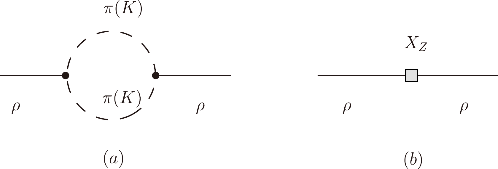
Figure A1. Feynman diagrams contributing to ρ self-energy.
$ \begin{aligned}[b] {\cal L}_{4Y} =& \frac{X_{Y_1}}{2} \, \langle \nabla^2 V^{\mu\nu} \left\{\nabla_\nu,\nabla^\sigma\right\} V_{\mu\sigma} \rangle \\& + \frac{X_{Y_2}}{4} \, \langle \left\{\nabla_\nu,\nabla_\alpha\right\} V^{\mu\nu} \left\{\nabla^\sigma,\nabla^\alpha\right\} V_{\mu\sigma} \rangle \\ & + \frac{X_{Y_3}}{4} \, \langle \left\{\nabla^\sigma,\nabla^\alpha\right\} V^{\mu\nu} \left\{\nabla_\nu,\nabla_\alpha\right\} V_{\mu\sigma} \rangle\, . \end{aligned}\tag{A14} $

Specifically, only the combination of couplings
$X_Y\equiv X_{Y_1}+ X_{Y_2}+ X_{Y_3}\equiv X_Y^r+\delta X_Y$ is relevant for this purpose. Using Lagrangians in Eqs. (12) and (A14), ρ self-energy takes the form:$ \begin{aligned}[b] \Sigma_{\rho}(p^2) =& -\frac{G_V^2}{48F^4\pi^2 } p^4\Bigg\{\left(1-\frac{6m_\pi^2}{p^2}\right)\left(\lambda_{\infty}-\ln\frac{m_\pi^2}{\mu^2}\right)\\&-\frac{8m_\pi^2}{p^2} -\sigma_\pi^3\ln\left(\frac{\sigma_\pi+1}{\sigma_\pi-1}\right)\\ &+\left(1-\frac{6m_K^2}{p^2}\right)\left(\lambda_{\infty}-\ln\frac{m_K^2}{\mu^2}\right)-\frac{8m_K^2}{p^2} \\&-\sigma_K^3\ln\left(\frac{\sigma_K+1}{\sigma_K-1}\right)+\frac{10}{3}\Bigg\}-X_Y p^4\,. \end{aligned}\tag{A15} $

The renormalized ρ mass fulfills:
$ M_\rho^2=M_V^2+\Sigma_{\rho}(M_\rho^2)\,. \tag{A16}$

Given that physical
$ M_\rho $ is finite, the following holds:$ \delta X_Y=-\frac{G_V^2}{48F^4 M_\rho^2\pi^2 }\left(1-6\frac{m_\pi^2}{M_\rho^2}-6\frac{m_K^2}{M_\rho^2}\right)\lambda_{\infty}\,. \tag{A17} $

The wave-function renormalization constant of ρ meson is obtained from:
$ Z_\rho=1+\frac{\partial \Sigma_\rho(p^2)}{\partial p^2}\bigg|_{p^2=M_\rho^2}\,. \tag{A18} $

In our calculation of
$ \rho-\omega $ mixing, the tree amplitudes can only absorb the ultraviolet divergence that is proportional to$ p^0 $ . To neutralize$ O(p^2) $ ,$ O(p^4) $ , and$ O(p^6) $ ultraviolet divergence originating from loop contribution$ S_{\rho\omega}^{(c)} $ ,$ S_{\rho\omega}^{(d)} $ ,$ S_{\rho\omega}^{(e)} $ , and$ E_{\rho\omega}^{\pi\gamma} $ , we construct the counterterms as follows:$ \begin{aligned}[b] {\cal L}_{ct}=&Y_A\langle V_{\mu\nu}V^{\mu\nu}\chi_+\rangle -\frac{1}{2}Y_B\langle \nabla^{\lambda}V_{\lambda\mu}\nabla_{\nu}V^{\nu\mu}\chi_+\rangle \\ &+\frac{Y_{C_1}}{2}\langle \nabla^2V^{\mu\nu}\{\chi_+,\{\nabla_\nu,\nabla^\sigma\}V_{\mu\sigma}\}\rangle \\ &+\frac{Y_{C_2}}{4}\langle \{\nabla_\nu,\nabla_\alpha\}V^{\mu\nu}\{\chi_+,\{\nabla^\sigma,\nabla^\alpha\}V_{\mu\sigma}\}\rangle \\ &+\frac{Y_{C_3}}{4}\langle \{\nabla^\sigma,\nabla^\alpha\}V^{\mu\nu}\{\chi_+,\{\nabla_\nu,\nabla_\alpha\}V_{\mu\sigma}\}\rangle \\ &+\frac{Z_A F_V}{2\sqrt{2}}\langle V_{\mu\nu}f_+^{\mu\nu}\rangle +\frac{Z_B F_V}{2\sqrt{2}}\langle V_{\mu\nu}\nabla^{2}f_+^{\mu\nu}\rangle \\ &+\frac{Z_C F_V}{2\sqrt{2}}\langle V_{\mu\nu}\nabla^{4}f_+^{\mu\nu}\rangle +\frac{Z_D F_V}{2\sqrt{2}}\langle V_{\mu\nu}\nabla^{6}f_+^{\mu\nu}\rangle \,. \end{aligned}\tag{A19} $

We adopt
$ \overline{\rm MS}-1 $ subtraction scheme and absorb the divergent pieces proportional to$ \lambda_\infty $ by the bare couplings in the counterterms. Consequently, the remanent finite pieces of counterterms can be expressed as$ \Pi_{\rho\omega}^{ct}=X_W^r\, p^6+X_Z^r\,p^4+X_R^r\, p^2 \ , \tag{A20} $

with
$ \begin{aligned}[b] X_W^r\equiv& \frac{8\pi\alpha F_\rho F_\omega}{3}(Z_D^r +Z_B^r Z_C^r)\ ,\\ X_Z^r\equiv& \frac{4\pi\alpha F_\rho F_\omega}{3}(2 Z_C^r +{Z_B^r}^2)\\ &+16M_\rho(m_u-m_d)(Y_{C_1}^r+Y_{C_2}^r+Y_{C_3}^r)\ ,\\ X_R^r\equiv&\frac{8\pi\alpha F_\rho F_\omega}{3}Z_B^r-4M_\rho(m_u-m_d)Y_B^r\ . \end{aligned}\tag{A21} $

In summary, at the NLO in
$ 1/N_C $ , the UV-renormalized mixing amplitude is as follows:$ \begin{aligned}[b] {\Pi}^r_{\rho\omega}(p^2)=& S_{\rho\omega}^{(a)}\sqrt{Z_\rho}+\bar{S}_{\rho\omega}^{(c)}+\bar{S}_{\rho\omega}^{(d)}+\bar{S}_{\rho\omega}^{(e)}+\overline{E}_{\rho\omega }^{\pi\gamma}(p^2)\\&+X_W^r p^6+ X_Z^rp^4+X_R^rp^2\,, \end{aligned}\tag{A22} $

where a bar denotes that the divergences are subtracted.
As discussed in Ref. [41], the mixing amplitude should vanish as
$ p^2\to 0 $ . Thus, the final expression of the renormalized mixing amplitude is obtained as follows:$ {\Pi}_{\rho\omega}(p^2)={\Pi}^r_{\rho\omega}(p^2)-{\Pi}^r_{\rho\omega}(0)\ , \tag{A23}$

where an additional finite shift is imposed to guarantee that constraint
$ {\Pi}_{\rho\omega}(0)=0 $ is satisfied. It should be noted that due to the finite shift performed in Eq. (A23), our numerical calculation is actually independent of the coupling$ X_Y^r $ . In our numerical computation, scale μ will be set to$ M_\rho $ , and we use$ (m_u-m_d)=-2.49 $ MeV provided by PDG [44].
Momentum dependence of $ {\boldsymbol{\rho-\omega}} $ mixing in the pion vector form factor and its effect on ${\boldsymbol{(g-2)_\mu}} $
- Received Date: 2023-03-14
- Available Online: 2023-10-15
Abstract: The inclusion of the


 DownLoad: