


 Abstract
 HTML
HTML Reference
 Related
 PDF
PDF


-
Gravitational waves, which in physics refer to the ripples in the curvature of space-time, travel outward from a source of radiation in the form of waves that transmit energy through gravitational radiation. In other words, a gravitational wave is a kind of wave produced by the violent movement and change in matter and energy. Einstein predicted the existence of gravitational waves in general relativity, which is a consequence of the Lorentz invariance of general relativity [1−6]. To date, except for the GW detectors in low and middle frequency bands (such as: BICEP3 [7], Ali [8, 9], PTA [10], LISA [11−13], Taiji [14, 15], TIANQIN [16, 17], DECIGO [12, 18], LIGO [19−23]), several instruments have been built to detect high-frequency gravitational waves (HFGW). However, the abovementioned sensors do not have sufficient sensitivity for the detection of high-frequency gravitational waves [24]. In this paper, we will discuss another type of detector for the detection of very high frequency GWs of about 1 GHz. The goal is to supplement the detection of GW signals in all frequency bands.
There have been many researches on the calculation of Li-Baker detector. Li et al. [25−31] studied the response of electro-magnetic field to high-frequency relic gravitational waves (HFRGWs) by using a Gaussian beam propagating through a static magnetic field . Based on this, Li et al. [32, 33] further researched the calculation of signal (i.e. PPF) and noise (i.e. BPF) in the sycro-resonance electromagnetic system, which consists of a standard Gaussian beam (GB), a static magnetic field, and fractal membranes . In particular, Wen et al. [34, 35] found that the Li-Baker detector can observe polarizations other than those predicted by general relativity.
Following the above studies, Wei et al. proposed some improvements. Their main innovation was replacing the standard GB by a modulated GB with bandwidth. In addition, they used deep learning for data processing [36]. Their results showed that in random thermal noise, the signal (PPFs) can be recongnized correctly by convolutional neural networks (CNN), and the parameters estimation was also accurate. However, in an actual experiment, the noise is more complicated than just thermal noise. Therefore, in this study, we investigated the detectability of PPFs in the noise composed of BPFs (main noise), diffraction noise, and shot noise. Furthermore, we used traditional data processing to analyze the signal to noise ratio (SNR) and detectable areas.
The paper is structured as follows: (1) In Sec. II, we briefly introduce the principle of the detector. (2) The accurate expression and physical behavior of the first-order transverse perturbative photon fluxes, background photon fluxes, and other system noise are discussed in Secs. III, IV, and V, respectively. (3) The processing of the signal and noise data to obtain the SNR by using matched filter and other methods is discussed in Sec. VI. Finally, the discussion and conclusion are presented, including some meaningful remarks and some suggestions for further research.
-
When a gravitational wave and electromagnetic field exist together, it is equivalent to the electromagnetic field in curved space-time, so we need to consider the electrodynamic equation of curved space-time, which can be explained by the electro-dynamical equations in curved space-time [25, 26, 28, 29, 34],
$ \begin{equation} \frac{-1}{\sqrt{-g}}\frac{\partial}{\partial x^\nu}(\sqrt{-g}g^{\mu \alpha}g^{\nu \beta}F_{\alpha \beta})=\mu_0J^\mu, \end{equation} $

(1) $ \begin{equation} \nabla_\alpha F_{\mu \nu}+\nabla_\nu F_{\alpha \mu}+\nabla_\mu F_{\nu \alpha}=0, \end{equation} $

(2) where
$ J^\mu $ indicates the four-dimensional electric current density. We consider the detector in vacuum, so$ J^{\mu}=0 $ . Also,$ g^{\mu \nu} $ is the contra-variant metric. All of$ F_{\alpha \beta} $ ,$ F_{\mu \nu} $ ,$ F_{\alpha \mu} $ , and$ F_{\nu \alpha} $ are co-variant tensors. Because the source of the gravitational wave is so far away from the observation point that the metric of HFGWs can be written as a small perturbation$ h_{\mu \nu} $ to the flat space-time$ \eta_{\mu \nu} $ ,$ \begin{equation} g_{\mu \nu}=h_{\mu \nu}+\eta_{\mu \nu}. \end{equation} $

(3) Supposing an ideal condition, the HFGWs are along the z axis in our coordinate system, and considering the TT-gauge [25, 30, 31, 35], the HFGWs can be expressed in two polarizations as
$h_{11}=-h_{22}= A_{\oplus}\exp[{\rm i}(k_{g}z- \omega_{g}t)]$ ,$h_{12}=h_{21}={\rm i}A_{\otimes}\exp[{\rm i}(k_{g}z-\omega_{g}t)]$ . Here,$ A_{\otimes} $ and$ A_{\oplus} $ denote the amplitude of the$ \oplus $ and$ \otimes $ polarizations in the laboratory frame, respectively. Moreover, in a curved space-time, if there is a static magnetic field that is perpendicular to the direction of gravitational wave propagation, then an electromagnetic response will be generated. If the high-level minima is ignored, we could get the components of first-order disturbed electromagnetic field as follows [25, 29]$ \begin{aligned}[b] \widetilde{E}_x^1(z,t,\omega_{g})=&\frac{\rm i}{2}A_{\oplus}\widehat{B}_y^0k_gc(z+l_1)\exp[{\rm i}(k_gz-\omega_{g}t)]\\ &+\frac{1}{4}A_{\oplus}\widehat{B}_y^0c\exp[{\rm i}(k_gz+\omega_{g}t)], \end{aligned} $

(4) $ \begin{aligned}[b] \widetilde{B}_y^1(z,t,\omega_{g})=&\frac{\rm i}{2}A_{\otimes}\widehat{B}_y^0k_gc(z+l_1)\exp[{\rm i}(k_gz-\omega_{g}t)]\\ &-\frac{1}{4}A_{\otimes}\widehat{B}_y^0\exp[{\rm i}(k_gz+\omega_{g}t)], \end{aligned} $

(5) $ \begin{aligned}[b] \widetilde{E}_y^1(z,t,\omega_{g})=&-\frac{1}{2}A_{\oplus}\widehat{B}_y^0k_gc(z+l_1)\exp[{\rm i}(k_gz-\omega_{g}t)]\\ &+\frac{\rm i}{4}A_{\oplus}\widehat{B}_y^0c\exp[{\rm i}(k_gz+\omega_{g}t)], \end{aligned} $

(6) $ \begin{aligned}[b] \widetilde{B}_x^1(z,t,\omega_{g})=&\frac{1}{2}A_{\otimes}\widehat{B}_y^0k_gc(z+l_1)\exp[{\rm i}(k_gz-\omega_{g}t)]\\ &+\frac{\rm i}{4}A_{\otimes}\widehat{B}_y^0\exp[{\rm i}(k_gz+\omega_{g}t)], \end{aligned} $

(7) $ \begin{align} \widetilde{E}_z^1(z,t,\omega_{g})=\widetilde{B}_z^1(z,t,\omega_{g})=0. \end{align} $

(8) In this expression,
$ l_1=0.3m $ , the superscripts 0 and 1 denote the quantity of the background field and disturbance field, respectively, and the notations$ \sim $ and$ \land $ denote the time-dependent evolution field and static field, respectively.In order to increase the energy of the perturbed electromagnetic field, we add a Gaussian beam to provide a zero-order perturbed electromagnetic field, which was proposed by Li-Baker [31]. Typically, a Gaussian beam resonance scheme, called as the Li-Baker detector, is used to detect HFGWs in the GHz band [25, 31]. The basic structure of the detector is shown in Fig. 1.
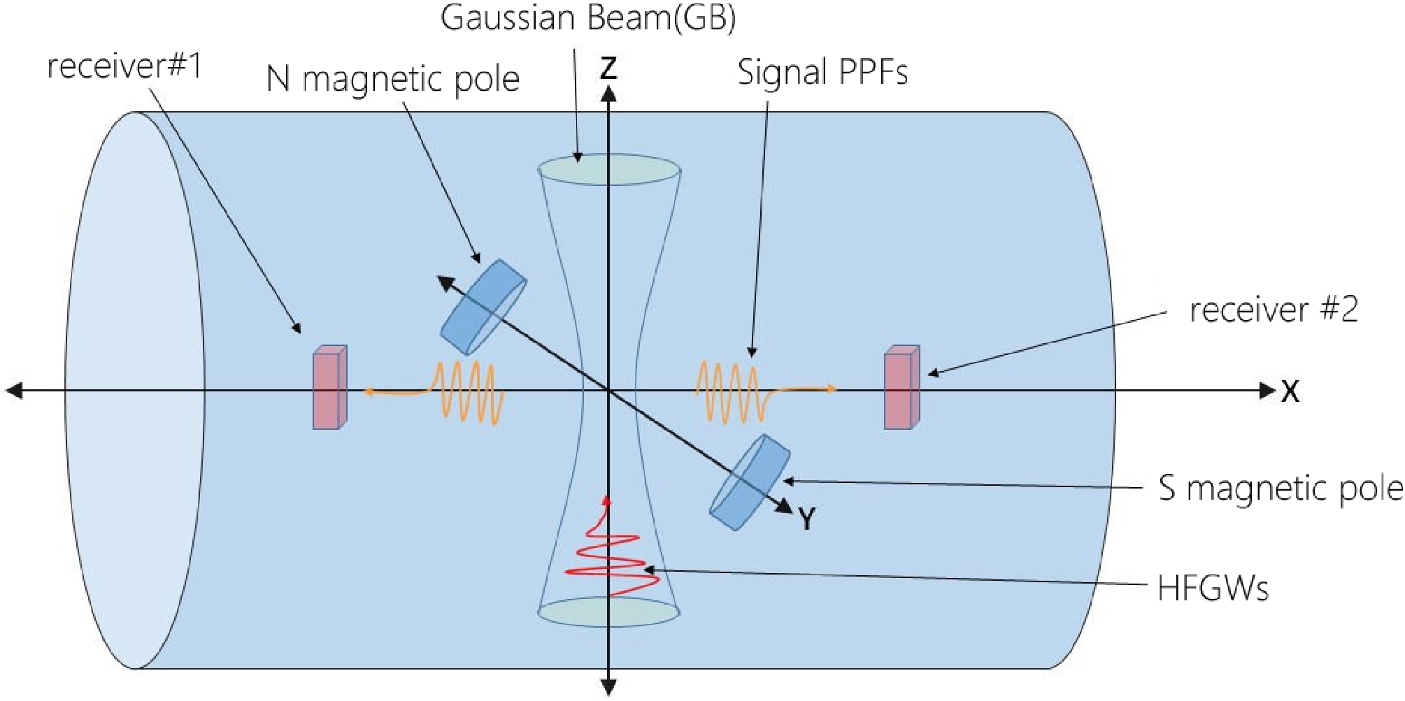
Figure 1. (color online) Schematic diagram of the detector structure [37]. Here, the receivers are used to receive the photon fluxes along the x axis.
In Fig. 1, the static magnetic field
$ \widehat{B}_y^0 $ on the y axis would interact with the incoming HFGWs and generate a first order perturbative EM signal [25, 26, 28, 32], which will be discussed in the next section. -
Without loss of the generality, we assume a standard Gaussian beam (GB) [25] as
$ \begin{aligned}[b] \widetilde{\Psi}(x,y,z,\omega_{e})=&\frac{\psi_0}{\sqrt{1+\left(\dfrac{z}{z_o}\right)^2}}\exp\left(-\frac{r^2}{W^2}\right)\\ & \times \exp\Bigg\{{\rm i}[k_ez-\omega_{e}t-\tan^{-1}\left(\frac{z}{z_0}\right)+\frac{k_e r^2}{2R}+\delta\Bigg\}. \end{aligned} $

(9) In the above equation,
$ \psi_0 $ is the maximum amplitude of the electric field component of the Gaussian beam along the direction. Here,$ W=W_0\sqrt{(1+(z/z_0)^2)} $ , with$ W_0 $ being the waist radius of the Gaussian beam, and$ r^2=x^2+y^2 $ ;$ k_e=2\pi/\lambda_e $ is the wave number; and$ R=z+z_0^2/z $ is the curvature radius of the wave fronts of the GB at$ z=0 $ . Also,$ \omega_e=k_e c $ ,$ z_0=\pi W_0/\lambda_e $ , and δ is the initial phase of the Gaussian beam. In this paper, we set$ \psi_0=1260 $ (the corresponding power of the laser is about 10 W),$ \delta=1.32π $ , and$W_0=0.06~\rm m$ . The static magnetic field is assumed to be distributed in the following region: ($ l_1<z<l_2 $ ,$l_1=0.3~\rm m$ ,$l_2=5.7~\rm m$ ).However, in practice, the Gaussian beam cannot be strictly monochromatic, but has a frequency band with the set frequency as the center frequency. As a result, the background Gaussian beam in a certain frequency range near the center frequency can resonate with the gravitational wave in the corresponding frequency band and generate a first-order transverse PPF, which also has the corresponding bandwidth. Therefore, the results of previous related work can be further modified to be more consistent with reality. Therefore, we added an additional item
$ \exp[-\dfrac{(t-\tfrac{\beta}{f_e})^2}{f_e^\alpha }] $ to the expression of the monochromatic GB [36], so that the expression of GB is as follows:$ \begin{aligned}[b] \widetilde{\Psi}_{real}(x,y,z,\omega_{e})=&\frac{\psi_0}{\sqrt{(1+{\frac{z}{z_0}}^2 )}}\exp\left(-\dfrac{r^2}{W^2}\right)\exp\left[-\frac{(t-\frac{\beta}{f_e})^2}{f_e^\alpha }\right]\\ & \times \exp\Bigg\{{\rm i}\Bigg[k_e z-\omega_e t-\tan^{-1}\frac{z}{z_0}+\frac{(k_e r^2)}{2R}+\delta\Bigg]\Bigg\}. \end{aligned} $

(10) Through parameter test, in order to achieve the desired modulation effect, we set
$ \alpha=-2.0 $ and$ \beta=0.5 $ through a parameter test. We compare the difference between the standard GB and the modulated GB in frequency domain (Figs. 2 and 3).
Figure 2. (color online) Distribution of amplitude with frequency for the modulated GB and standard GB; the amplitude is normalized.
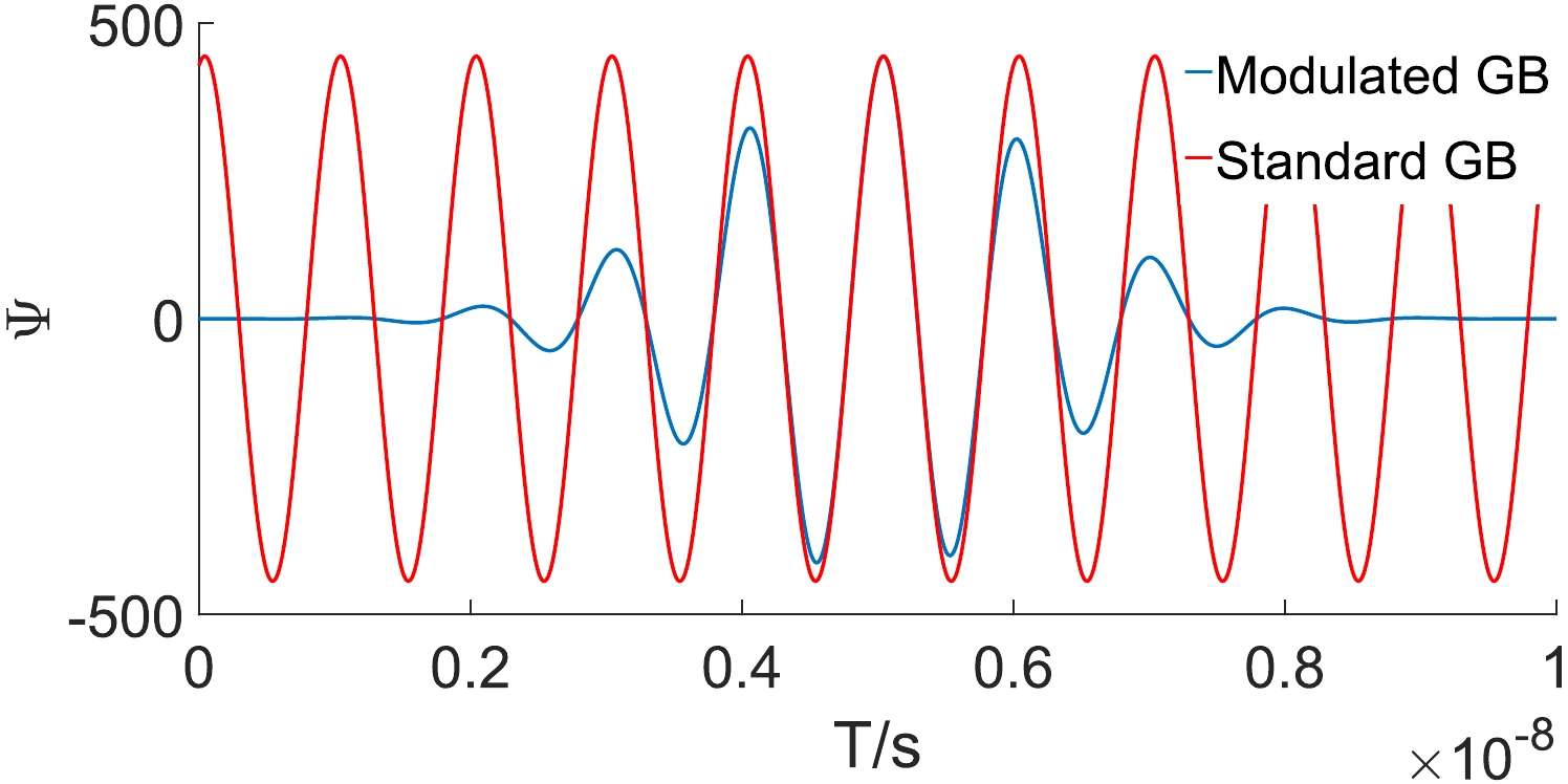
Figure 3. (color online) The amplitude of the modulated GB and standard GB with time.
We can find that the spectrum of the modulated GB is consistent with our expection, and the band width is approximately 0.32 GHz. The part of the frequency band where the corresponding energy reaches more than half of the central frequency energy is selected as the effective bandwidth, which is set to be the frequency band in our simulation. For simplifying our calculation and maintaining the physics mechanism, we suppose that the electric field in the z direction is zero. Then, using the condition of non-divergence,
$ \nabla\cdot E=\partial\psi_x/\partial x+\partial\psi_y/\partial y=0 $ and$\widetilde{B}^0=-\dfrac{\rm i}{\omega}\nabla\times\widetilde{E}^0$ . Without loss of generality, we choose each component of the background electromagnetic field as$ \widetilde{E}_x^0=\widetilde{\psi}_{\rm real}, \widetilde{E}_z^0=0 $ [25, 33]. Then, the other electromagnetic field components can be obtained by solving Maxwell's equations in flat space-time [25, 25, 28]:$ \begin{equation} \widetilde{E}_y^0(x,y,z,t,\omega_{e})=2x\left(\frac{1}{W^2}-\frac{{\rm i} k_e}{2R}\right)\int\widetilde{E}_x^0 {\rm d} y, \end{equation} $

(11) $ \begin{equation} \widetilde{B}_x^0(x,y,z,t,\omega_{e})=\frac{\rm i}{\omega_{e}}\frac{\partial\widetilde{E}_y^0 }{\partial z}, \end{equation} $

(12) $ \begin{equation} \widetilde{B}_y^0(x,y,z,t,\omega_{e})=\frac{\rm i}{\omega_{e}}\frac{\partial\widetilde{E}_x^0 }{\partial z}, \end{equation} $

(13) $ \begin{equation} \widetilde{B}_z^0(x,y,z,t,\omega_{e})=\frac{\rm i}{\omega_{e}}\left(\frac{\partial\widetilde{E}_x^0 }{\partial y}-\frac{\partial\widetilde{E}_y^0}{\partial x}\right). \end{equation} $

(14) Here, we only list the computational components involved in the simulation experiment. Since these two formulas involve special functions that cannot be solved analytically, we only performed numerical calculations for the relevant formulas in our work. For the Gaussian beam, it will generate the Poynting vectors, which are the BPFs. The physical behavior of the longitudinal photon fluxes can hardly be distinguished before and after the existence of gravitational waves [32, 35]; therefore, in the following content, we focus on the transverse (x direction) photon fluxes. When there is no gravitational wave, the transverse photon fluxes as follows:
$ \begin{equation} \widetilde{n}_x^0(x,y,z,t,\omega_{e})= \frac{1}{\hbar\omega_{e}}<\frac{1}{\mu_0}(\widetilde{E}_y^0\widetilde{B}_z^0)> =\frac{1}{2\hbar\omega\mu_0}{\rm Re} [\widetilde{E}_y^0\times\widetilde{B}_z^0]. \end{equation} $

(15) Here, <> means the average over a period of time, and
$ \widetilde{E}_y^0, \widetilde{B}_z^0 $ are the y component of the background electric field and the z component of the magnetic field, respectively; both of them can be solved using Maxwell's equations of electrodynamics in curved space-time [25, 25, 33]. The specific calculation of$ \widetilde{n}_x^0 $ will be discussed in detail in Sec. IV.When there are gravitational waves,
$ \widetilde{B}_z^0 $ of the background field will be coupled with the first-order transverse perturbed electrical component (see Eq. (6)) mentioned above ($ w_e=w_g $ ), thus forming the perturbed photon fluxes as follows:$ \begin{equation} \widetilde{n}_x^1(x,y,z,t,\omega)= \frac{1}{\hbar\omega_{e}}<\frac{1}{\mu_0}(\widetilde{E}_y^1\widetilde{B}_z^0)> =\frac{1}{2\hbar\omega\mu_0}{\rm Re} [\widetilde{E}_y^1\times\widetilde{B}_z^0]. \end{equation} $

(16) Set
$ t=t_d $ ($ t_d $ indicates the beginning of signal accumulation), and after the accumulation for a period of time$ t_0 $ , the number of signal photons received by the receivers, which is parallel to the$ yoz $ plane and is placed on the x axis, can be obtained by integration:$ \begin{equation} \widetilde{N}_x^1(x,t_d)={\rm Re} \left[\int_{t_d}^{t_d+t_0}\iint_{a_r}\widetilde{n}_x^1(x,y,z,t,\omega){\rm d}y{\rm d}z{\rm d}t\right]. \end{equation} $

(17) Here,
$ \widetilde{N}_x^1(x,t_d) $ represents the PPF. In the simulation, the area of the receiving plane was set as$a_r=\Delta y \Delta z= 0.01~\rm m^2$ . The dimensionless amplitude of the gravitational wave is$ 1.0\times10^{-31} $ [25, 36], and the frequency of the gravitational wave and the center frequency of the background electromagnetic wave are chosen to be$f_e=f_g=10^9 ~{\rm Hz}$ . The signal accumulation time is set as$t_0=1.3\times10^{-10}~{\rm s}$ . The spatial and temporal distribution of the PPF$ \widetilde{N}_x^1(x,t_d) $ with x (the transverse coordinate position of the receiving plane) and$ t_d $ (the initial time of detection) are shown in Fig. 4.
Figure 4. (color online) The number of PPF varying x and
$ t_d $ ; the detection area is in the region of$y\in[-0.05,0.05]~ {\rm m}, $ $ z\in[-0.05,0.05] {~\rm m}$ .The power of PPF is
$ \begin{equation} P_{\rm PPF}=h\nu_e\widetilde{N}_x^1(x,t_d). \end{equation} $

(18) It is obvious that if we fix the position of the detector (x) and accumulate the signal at
$t_d=0.5\times10^{-8}~{\rm s}$ from the beginning of the generation of the PPF, the number of PPFs will reach the maximum. Then, if we fix the initial time of signal accumulation ($ t_d $ ) and place the detector at the position ($ x=0 $ ), the signal photon fluxes will reach the maximum, and the number of photons decays with the increase in the transverse distance (|x|). The number of PPFs reaches the maximum, which is 2700 at$(0~\rm m,0.5\times 10^{-8}~{\rm s})$ , while the$P_{\rm PPF}$ can reach up to$1.789\times10^{-21}~\rm W$ . -
In the above mentioned, GB will generate BPF, which will seriously interfere the detection of the PPF. Therefore, we will discuss BPF on the x axis as the main noise of the system in this section. According to the literature [25−27], the density of the BPF in the Li-Baker detector can be described as Eq. (15). The analytic formulas of
$ \widetilde{E}_y^0(x,y,z,t) $ and$ \widetilde{B}_z^0(x,y,z,t) $ are given below:$ \begin{aligned}[b] \widetilde{E}_y^0(x,y,z,t,\omega_{e})=&\frac{2x\psi_0}{\sqrt{1+\frac{z^2}{f^2}}}\left(\frac{1}{W^2}-\frac{{\rm i} k_e}{2R}\right)\\& \times \exp\left[{\rm i}\left(k_ez-\omega_{e}t-\arctan\frac{z}{f}+\frac{k_er^2}{2R}+\delta\right)\right] \end{aligned} $

$ \times\exp\left[-x^2\left(\frac{1}{W^2}-\frac{{\rm i}k_e}{2R}\right)\right]\int\exp\left[y^2\left(\frac{1}{W^2}-\frac{{\rm i}k_e}{2R}\right)\right]{\rm d} y, $

(19) $ \begin{aligned}[b] \widetilde{B}_z^0=&\frac{{\rm i} \psi_0}{\omega_{e}\sqrt{1+\frac{z^2}{f^2}}}\exp\left[-\frac{(t-\frac{\beta}{f_e})^2}{f_e^\alpha }\right] \\& \times\exp\left[{\rm i}\left(k_ez-\omega_{e}t-\arctan\frac{z}{f}+\frac{k_er^2}{2R}+\delta\right)\right]\\ &\times\Bigg\{2\left(\frac{-1}{W^2}+\frac{{\rm i}k_e}{2R}\right)\times y\exp\left[\left(\frac{-1}{W^2}+\frac{{\rm i}k_e}{2R}\right)r^2\right]\\&+4x^2{\left(\frac{-1}{W^2}+\frac{{\rm i}k_e}{2R}\right)}^2\\ &\times\int\exp\left[\left(\frac{-1}{W^2}+\frac{{\rm i}k_e}{2R}\right)r^2\right]{\rm d}y-2\left(\frac{1}{W^2}-\frac{{\rm i}k_e}{2R}\right)\\ &\times\int\exp\left[\left(\frac{-1}{W^2}+\frac{{\rm i}k_e}{2R}\right)r^2\right]{\rm d}y\Bigg\}. \end{aligned} $

(20) Therefore, the number of BPF photons received by the receiver should be
$ \begin{equation} \widetilde{N}_x^0(x,t_d)={\rm Re} \left[\int_{t_d}^{t_d+t_0}\iint_{a_r}\widetilde{n}_x^0(x,y,z,t,\omega){\rm d} y{\rm d}z{\rm d}t \right]. \end{equation} $

(21) Then, the power of BPF is
$ \begin{equation} P_{\rm BPF}=h\nu_e\widetilde{N}_x^0(x,t_d). \end{equation} $

(22) As shown in Fig. 5, the intensity of BPF at the optical waist is zero, and it increases first and then decays rapidly with the increase in the transverse distance x. The number of PPFs reaches the maximum, which is
$ 1.57\times10^{27} $ at$(0.341~{\rm m},~0.5\times10^{-8}{\rm s})$ while$P_{\rm PPF}$ can reach up to$1.04\times10^3~\rm W$ . The direction of BPF will be discussed in Sec. VI.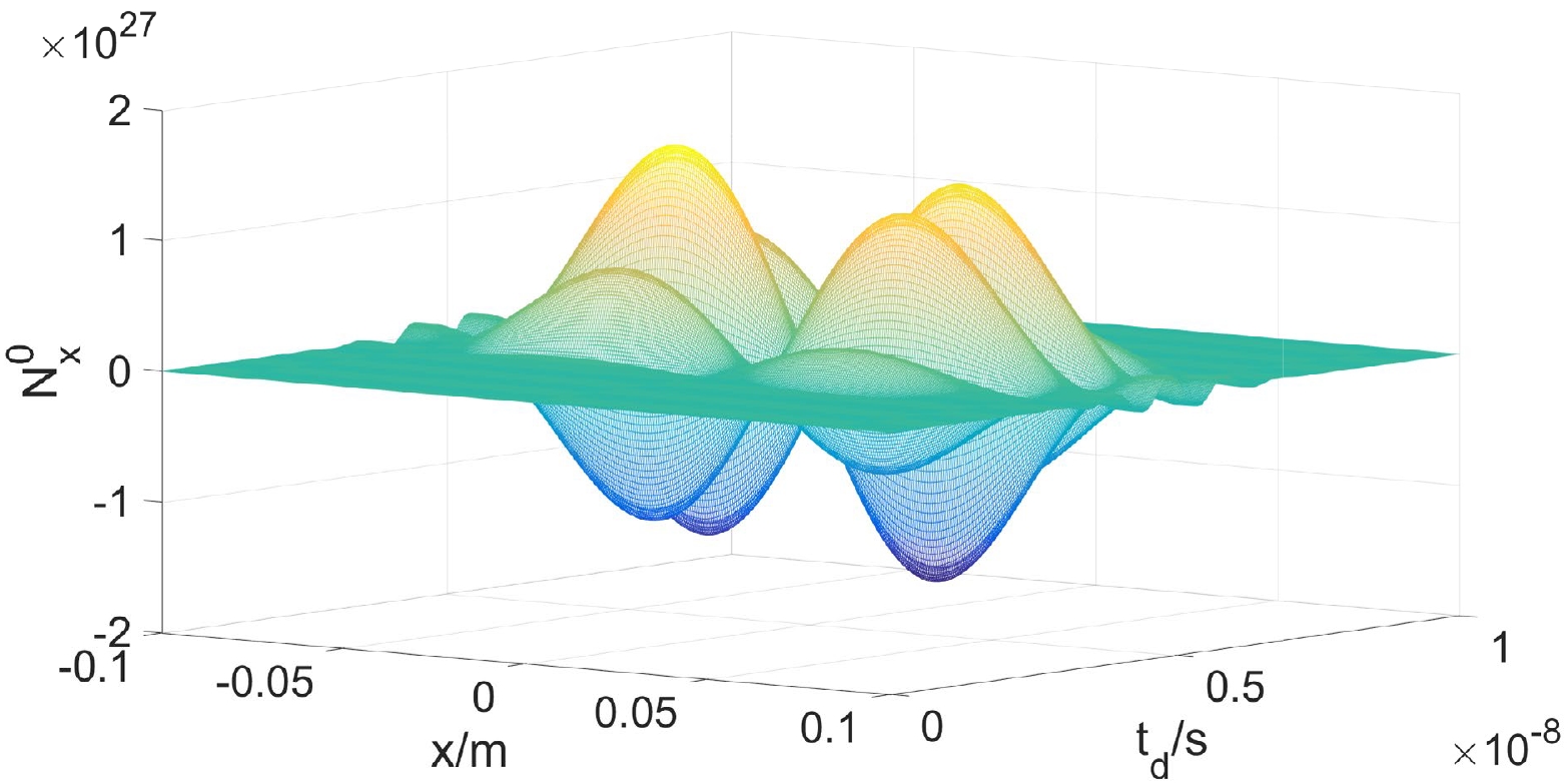
Figure 5. (color online) The number of BPF varying x and
$ t_d $ ; the detection area is in the region of$y\in[-0.05,0.05]~{\rm m}, $ $ z\in[-0.05,0.05]~{\rm m}$ , and the negative part indicates that the photon flux is in the negative x direction. -
In addition to BPF, we discuss diffraction noise and shot noise. When the Gaussian beam propagates along the z direction, the structure of the Gaussian beam generator causes the GB to diffract in the x direction, and it is called diffraction photon flux. This is a potential problem for the design of Li-Baker detectors because the diffraction signal could overwhelm the microwave receiver or represent an important external source of granular noise.
The density of diffraction noise photon fluxes along x axis is expressed as [25, 26, 37]:
$ \begin{equation} n_{\rm dif}=k_e^2(W_0^2/32d^2)\exp\left(-\frac{1}{2}k_e^2W_0^2\right)a_rn_{\rm GB}. \end{equation} $

(23) In Eq. (23),
$ k_e=\dfrac{2\pi}{\lambda_e} $ ,$ n_{\rm GB} $ is the photon flux of the Gaussian beam, i.e., BPF, and d represents the distance from the waist of the Gaussian beam to the receiver. Then, the number of diffracted noise photons that eventually hit the receiving plane could be expressed as:$ \begin{equation} N_{r\,\rm dif}=n_{\rm dif}[a_r/(l\pi d)]\varepsilon_{ab}. \end{equation} $

(24) Here, l represents the length of the GB (
$\; 0.3~\rm m$ for the nominal case), and$ \varepsilon_{ab} $ represents the wall absorption coefficient (the wall absorption coefficient has been discussed and calculated in the literature [25, 29, 30]).According to the literature [30], we set the wall absorption coefficient
$ \varepsilon_{ab}=10^{-22} $ .Figure 6 shows the relationship between the received photon number of diffraction noise (
$N_{r\,\rm dif}$ ) and the position of the receiver (x); here, d is within 10 radii of the optical waist$(-0.6~{\rm m}\le d\le 0.6~{\rm m})$ . It is found that the number of diffraction photons is very small, which decays symmetrically to both sides of the optical waist. The corresponding power is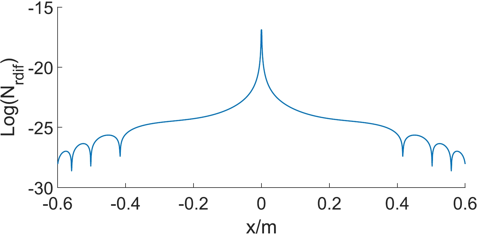
Figure 6. (color online) The distribution of diffraction noise with x,
$N_{r\,\rm dif}$ is converted to logarithm. Here$ \varepsilon_{ab}=10^{-22} $ ,$-0.6~{\rm m}\le d\le 0.6~{\rm m}$ .$ \begin{equation} P_{\rm dif}=h\nu_e{N_{r\,\rm dif}}. \end{equation} $

(25) In terms of Fig. 6, the maximum number of the diffraction photon fluxes can only be
$ 10^{-16} $ . This is obviously less than the PPFs and the other noises that we considered. Meanwhile, the maximum of$P_{\rm dif}$ can only be$10^{-40}~{\rm W}$ .Shot noise is a kind of statistical fluctuation that is generated from a sufficiently small number of particles in the output. In this study, we mainly explore two parts of shot noise: the shot noise
$ P_{nb} $ caused by BPF and the shot noise$ P_{ns} $ caused by PPF. Shot noise is proportional to the square root of the number of photons from the source; therefore, the noise energy can be expressed as [25, 26, 28, 37],$ \begin{equation} P_{nb}=h\nu_e\sqrt{{\widetilde{N}_x^0}}, \end{equation} $

(26) $ \begin{equation} P_{ns}=h\nu_e\sqrt{{\widetilde{N}_x^1}}, \end{equation} $

(27) $ \begin{equation} P_{tot}=P_{ns}+P_{nb}. \end{equation} $

(28) In our simulation, we set the position of the receiver as
$x=-0.08~\rm m,~ 0m,~ 0.06m$ . In Fig. 7,$ P_{ns} $ is much weaker than$ P_{\rm tot} $ . This is because$ P_{ns}\ll P_{nb} $ as$ {\widetilde{N}_x^1}\ll {\widetilde{N}_x^0} $ at the receiver positions. The maximum power of total shot noise is about$ 7.5\times10^{-15}~{\rm W} $ , which is larger than the signal (in the same condition, power of PPF is about$ 1.789\times10^{-21} $ W). Fortunately, due to the different propagation directions of BPF and PPF in some areas, we can neglect$ P_{nb} $ in those areas; then,$ P_{\rm tot}\thickapprox P_{ns}\sim 10^{-23}~{\rm W} $ . This will be discussed in the following section.
Figure 7. (color online) The power of shot noise generated by PPF (left subplot) and total transverse photon fluxes (right subplots) at
$x=-0.08~{\rm m},~ x=0~{\rm m},~ x=0.06~{\rm m}$ , with$ \Delta s=\Delta y \Delta z $ ($y\in[-0.05,0.05]~{\rm m}, z\in[-0.05,0.05]~{\rm m}$ ). -
In signal detection, SNR is critical. In order to obtain a greater SNR, we need to design an optimal linear filter. When the input signal of a linear time-invariant filter is a definite signal and the noise is additive stationary, the filter that can maximize the SNR is the matched filter, which matches the input signal.
Our signal (i.e, PPF) is a kind of determinate signal, and the noises are additive stationary; hence, according to the data processing theory, we just design a matched filter to enhance the SNR. In the matched filtering thory, the SNR of output is determined as
$ \begin{equation} SNR_o\le\int_{-\infty}^{\infty}\frac{|S(f)|^2}{P_n(f)}{\rm d} f. \end{equation} $

(29) When the response function
$ H(f) $ $ \begin{equation} H(f)=\frac{\alpha S^*(f)}{P_n(f)} {\rm e}^{-2\pi jft_0}, \end{equation} $

(30) $ \begin{equation} S(f)=FT[S(t)], \end{equation} $

(31) the
$ SNR_o $ will reach the maximum. Here,$ S(t) $ is the input signal of the filter in the time domain, and$ S(f) $ is the Fourier transform of the signal. In our work,$S(t)= P_{\rm PPF}\big|_{x=x_0}$ .$* $ indicates a complex conjugate and$ P_n(f) $ is the noise power spectrum. Here,$ \begin{equation} P_n=\sqrt{{P_{\rm BPF}}^2+{P_{ns}}^2+{P_{\rm dif}}^2}. \end{equation} $

(32) Figure 8 shows the BPF in the time domain and frequency domain, respectively. The position of the receiving screen is x = 0.08 m. In this location, the maximum number of noise photons is
$ 6.8\times10^{25} $ .
Figure 8. (color online)
$ \widetilde{N}_x^0 $ in the time domain and frequency domain. Here,$ x_0=0.08 $ m. In the left plot,$ f_e=1 $ GHz. The dashed lines represent the photons along the -x direction, which will not be recorded by the receiver. In the right plot,$ t_d=5\times10^{-9} $ s.Figure 9 shows the time and frequency domain diagrams of the PPF. When the receiver is fixed at x = 0.08 m, the maximum number of signal photons is
$ 700 $ .
Figure 9. (color online)
$ \widetilde{N}_x^1 $ in the time domain and frequency domain. Here,$ x_0=0.08 $ m. In the left plot,$ f_e=1 $ GHz. In the right plot,$ t_d=5\times10^{-9} $ s.It can be found that the BPF and PPF have different frequency spectrums. Based on the above equations, we derive the SNR to be only
$ 10^{-32} $ , which is too weak to be detected. That is mainly because the$P_{\rm BPF}$ far exceeds the signal and plays a dominant role in the noise (see Figs. 4, 5 and 7). In order to improve the SNR as much as possible, we must minimize the impact of BPF. Fortunately, we found an interesting result that the direction of the BPF changes with time, while the direction of PPF remains unchanged and always propagates along the positive direction of x axis. Because of this property, we propose a method to eliminate BPF, which is to locate the receiver at the transverse areas where the direction of BPF is opposite to that of PPF.By calculating the product of BPF and PPF with the location of the receiver (see Fig. 10), it is found that when the receiving plane is located within the transverse area (0.04 m, 0.082 m), we can remove the influence of the BPF. Therefore, we can also neglect the shot noise generated from the BPFs. Then, we analyze the SNR with the remaining noises. The result is shown in Table 1.

Figure 10. (color online) The directions of PPF and BPF varying with the receiver position x. Here,
$t_d=5\times10^{-8}~\rm s$ . A negative value (red areas) indicates that the directions of PPF and BPF are opposite, and a positive value (blue areas) indicates they are in the same direction.$ x_0 $ /m

$\rm PPF$ /

$\rm s^{-1} $ 

$N_{r\,\rm dif}$ /

$\rm s^{-1} $ 

$ N_{ns} $ /

$\rm s^{-1} $ 

SNR 0.040 453.6 $ 10^{-10} $ 

21 44 0.064 622 $ 10^{-14} $ 

25 320 0.080 197 $ 10^{-15} $ 

14 259 Table 1. Comparison of PPF,
$N_{r\,\rm dif}$ ,$ N_{ns}=\sqrt{\widetilde{N}_x^1} $ and SNR with the receiver located at$x_0=-0.04,~ 0.064,~ 0.08~\rm m$ .With the same receiver location (x = 0.08 m) where the receiver is beyond the GB waist, we calculate the signal power spectrum after matched filtering (Fig. 11). As shown in this figure, it is obvious that the power spectral density difference between the signal and noise is big enough to capture the signal in our target frequency range (GHz band). It can be seen that the SNR of the output after matched fitering has been improved to
$ 259 $ (see Table 1), which is expected to be detected.
Figure 11. (color online) The power spectral density of signal and noise.
-
In this study, considering the actual GB and all the possible noises, we compared the signal with all types of noise, and discussed how they differ in physical behaviors. The results are as follows: (1) in the time and space domains, the BPF and the PPF have different physical behaviors — the direction of PPFs remains unchanged, but the direction of BPF changes; (2) the amplitude of BPF is much more than that of PPF, but with the increase in x, the amplitude of BPF decreases faster than that of PPF. Therefore, we propose that the receiving screen can be placed at a specific location where the screen can only receive PPF and the other two noises. Under this condition, the SNR can be enhanced to 259 at
$x=0.08~\rm m$ , where the receiver will not interfere with the background electromagnetic field. This indicates that the detection of HFGW in the Li-Baker detector is feasible and the transverse size is maintained within 0.1 m.It should be noted that in order to perform detection, the required continuous scanning time should only be about
$5\times10^{-11}~\rm s$ (cf. Fig. 8). This can be realized using the current exposure technology. Nevertheless, in the actual experiment, the noise will be more complicated, but the total noise strength can be controlled once the BPF is eliminated.
Simulation of high-frequency gravitational wave detection using modulated Gaussian beam
- Received Date: 2023-05-12
- Available Online: 2023-10-15
Abstract: This paper investigates the feasibility of using a Li-Baker detector based on a modulated Gaussian beam to detect gravitational waves in the GHz band. The first-order perturbation photon fluxes (PPF, signal of the detector) and the background photon fluxes (BPF, main noise of the detector), which vary with time, and the transverse distance are calculated. The results show that their propagation directions and energy densities are much different in some areas. Apart from BPF, we also consider two other important noises: diffraction noise and shot noise. In the simulation, it is found that the diffraction noise and shot noise are both lower than the signal level. Meanwhile, the main noise (BPF) can be eliminated when the receiving screen is located in certain special transverse areas where the BPF direction is opposite to that of PPF. Thus, the signal to noise ratio (SNR) obtained using our detection method can reach up to


 DownLoad: