


 Abstract
 HTML
HTML Reference
 Related
 PDF
PDF


-
The standard model (SM) describes elementary particles and their interactions and is highly consistent with most current experimental results. However, it falls short in providing a complete explanation for the observed preponderance of matter over antimatter in the universe. The study of
$ CP $ violation provides a crucial perspective on understanding the origin and nature of this fundamental asymmetry, as well as exploring physics beyond the SM [1−3]. To date,$ CP $ violation has been discovered in the decay of mesons such as K [4], B [5, 6], and D [7] but not yet in any baryon decay.In 1956, Lee and Yang first proposed the violation of parity (P) in weak decays of baryons and later pointed out that violation of parity also implies a violation of charge (C) conjugation symmetry [8]. When studying the decays of a spin-1/2 hyperon Λ into a final state comprising a spin-1/2 baryon p and π, it is observed that the parity-even amplitude results in a p-wave state, whereas the parity-odd amplitude leads to an s-wave state. The amplitudes
$ P_{1} $ and$ S_{1} $ are used to denote the parity-even and parity-odd amplitudes, respectively. The decay parameters of baryons can be represented by the formula$\alpha=2\textstyle\frac{{\rm Re}(S_{1}*P_{1})}{|S_{1}|^{2}+|P_{1}|^{2}}$ . Theoretical physicists Donoghue and Pakvasa proposed that the observable quantity of$ CP $ violation could be constructed using asymmetric parameters in the decay of hyperons. They predicted that the$ CP $ violation of$ \Lambda \rightarrow p \pi^{-} $ in the SM is$ \mathcal O (10^{-5}) $ [9]. As a result, the decay of hyperons is sensitive to sources of$ CP $ asymmetry from physics beyond the SM [10]. In the$ CP $ -conserving limit, the amplitudes$ \bar{S_{1}} $ and$ \bar{P_{1}} $ for the charge-conjugated (c.c.) decay mode of the antibaryon$ \bar{\Lambda}\rightarrow \bar{p} \pi^{+} $ are$ \bar{S_{1}}=-S_{1} $ and$ \bar{P_{1}}=P_{1} $ . Therefore, the decay parameters$ \alpha_{-} $ ($ \Lambda \rightarrow p \pi^{-} $ ) and$ \alpha_{+} $ ($ \bar{\Lambda}\rightarrow \bar{p} \pi^{+} $ ) have opposite values, that is,$ \alpha_{-}=-\alpha_{+} $ .$ CP $ asymmetry can be described as$A_{CP}=\dfrac{\alpha_{-}+\alpha_{+}}{\alpha_{-}-\alpha_{+}}$ . If$ CP $ is conserved,$ A_{CP}=0 $ [11, 12].Experiments specifically aimed at observing hyperon
$ CP $ violation were conducted by Fermilab E756 [13] and HyperCP [14]. In these experiments, the sum of the observables$ A_{CP}^{\Xi^{-}}+A_{CP}^{\Lambda_{p}} $ for$ \Xi^{-} \rightarrow \Lambda \pi^{-} $ ($ \Xi^{-} $ ) and$ \Lambda \rightarrow p \pi^{-} $ ($ \Lambda_{p} $ ) was$ 0(7)\times10^{-4} $ [15]. The SM predicts that$ A_{CP}^{\Xi^{-}}+A_{CP}^{\Lambda_{p}} $ is$ -0.5\times10^{-4} \leq A_{CP}^{\Xi^{-}}+A_{CP}^{\Lambda_{p}} \leq -0.5\times10^{-4} $ [16]. In 2019, BESIII adopted an innovative method to study$ CP $ violation using hyperon-antihyperon pairs based on$ 1.3\times 10 ^{9}\; J/\psi $ and obtained the most accurate measurement results at that time,$ A_{CP}=-0.006\pm0.012\pm0.010 $ [17]. Subsequently, BESIII updated the result using 10 billion$ J/\psi $ events to$ A_{CP} = -0.0025 \pm 0.0046 \pm 0.0012 $ [18]. Nevertheless, the sensitivity of experiments to$ CP $ violation still does not meet theoretical predictions and is currently mainly limited by the statistical uncertainty [19, 20].The Super Tau-Charm Facility (STCF) is one of the most important accelerator-based particle physics large-scale scientific devices after the BEPCII collider [21]. The STCF was designed to collect over 1 ab
$ ^{-1} $ of data and has great potential in improving luminosity and realizing beam polarization. It is expected to provide$ 3.4 \times 10^{12} J/\psi $ events, and an electron beam polarization of 80-90$ % $ at$ J/\psi $ energy is expected to be achieved with the same beam current [22]. In this paper, we focus on the study of$ J/\psi \rightarrow \Lambda\bar{\Lambda} $ and show how the precision of the$ CP $ violation of Λ decay in$ J/\psi \rightarrow \Lambda\bar{\Lambda} \rightarrow p \bar{p}\pi^{+}\pi^{-} $ is related to the polarization of the electron beam. -
Currently, the STCF is in the research and design stage. The center-of-mass energy
$ (\sqrt{s}) $ designed for the STCF ranges from 2 to 7 GeV, with a peak luminosity of at least$ 0.5\times10^{35} $ cm$ ^{-2} $ s$ ^{-1} $ or higher at$ \sqrt{s}=4.0 $ GeV. Moreover, luminosity upgrade space will be left and the beam polarization operation of the second phase will be achieved. The STCF will serve as a crucial experiment to test the SM and study potential new physics.To manifest the expected high-precision with high-luminosity samples, the detector design of the STCF must meet the following requirements: a large coverage angle, high detection efficiency and good resolution of particles resulting in rapid triggering, and high radiation resistance. The preliminary design of the STCF detector mainly consists of a tracking system composed of inner and outer trackers, a particle identification (PID) system with
$ \pi/K $ and$ K/\pi $ misidentification of less than 2% with the PID efficiency of$ K/\pi $ over 97%, an electromagnetic calorimeter (EMC) with an excellent energy resolution and good position resolution, a super conducting solenoid, and a muon detector (MUD) that provides good$ \pi/\mu $ separation. Detailed requirements for each subdetector design can be found in Refs. [23, 24].A fast simulation software, specifically designed for STCF detectors, has been developed to investigate their physical potential and further optimize detector design [25]. Instead of simulating the objects in each subdetector using Geant4, the fast simulation models their response, including efficiency, resolution, and other factors used in data analysis, randomly sampling based on the size and shape of their performance. The performance of each subdetector for a given type of particle is described by empirical formulas. The scaling factor can be adjusted according to the performance limitations of the STCF detector, and these configurations can be easily interfaced. For this analysis, five groups of signal MC samples,
$ J/\psi \rightarrow \Lambda\bar{\Lambda} \rightarrow p \bar{p}\pi^{+}\pi^{-} $ , are generated according to the amplitude described in Sec. III and analyzed using the fast simulation package to investigate$ CP $ violation. Each group consists of$ 1.89 \times 10^8 J/\psi \rightarrow \Lambda \bar{\Lambda} $ events with the polarization rate of the electron beam ranging from 0 to 1, with a step size of 0.2. The obtained signal events are calculated using the following formula:$ \begin{equation} N_{\rm sig}=N_{J/\psi}\times \mathcal B_{J/\psi \rightarrow \Lambda\bar{\Lambda}}\times \mathcal B_{\Lambda\rightarrow p \pi^-} \times \mathcal B_{\bar{\Lambda}\rightarrow \bar{p} \pi^+}, \end{equation} $

(1) where
$N_{\rm sig}$ represents the number of signal events, and$ N_{J/\psi} $ represents the total number of$ J/\psi $ events as 0.1 trillion. Additionally,$ \mathcal B_{J/\psi \rightarrow \Lambda\bar{\Lambda}} $ ,$ \mathcal B_{\Lambda\rightarrow p \pi^{-}} $ , and$ \mathcal B_{\bar{\Lambda}\rightarrow \bar{p} \pi^{+}} $ denote the branching ratios of$ J/\psi \rightarrow \Lambda\bar{\Lambda} $ ,$ \Lambda\rightarrow p \pi^{-} $ , and$ \bar{\Lambda}\rightarrow \bar{p} \pi^{+} $ , with values of$ 1.89 \times 10^{-3} $ , 63.9%, and 63.9% [26], respectively. -
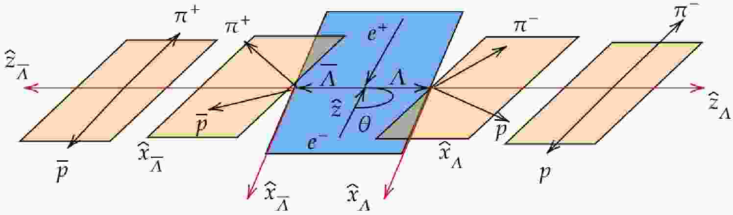
In electron-positron collision experiments, the polarization of the beam is reflected in the produced baryon-antibaryon pairs. The helicity frame is defined in Fig. 1. For the decay
$ J/\psi \rightarrow \Lambda\bar{\Lambda} $ , the$ \hat{z} $ axis follows the direction of the positron momentum. The$ \hat{z}_{1} $ axis is defined along the momentum vector of the Λ baryon, denoted by$ {p}_\Lambda $ =$ - {p}_{\bar{\Lambda}} $ =$ {p} $ in the center-of-mass system of the$ e^{+}e^{-} $ collision. The$ \hat{y}_{1} $ axis is perpendicular to the production plane and oriented along the vector$ {k}\; \times\; {p} $ , where$ {k}_{e^{-}} $ =$ - {k}_{e^{+}} $ =$ {k} $ is the momentum of the electron beam. The scattering angle of Λ is given by$ \cos\theta_{\Lambda} $ =$ \hat{ {p}} \cdot \hat{ {k}} $ , where$ \hat{ {p}} $ and$ \hat{ {k}} $ are unit vectors along the$ {p} $ and$ {k} $ directions, respectively.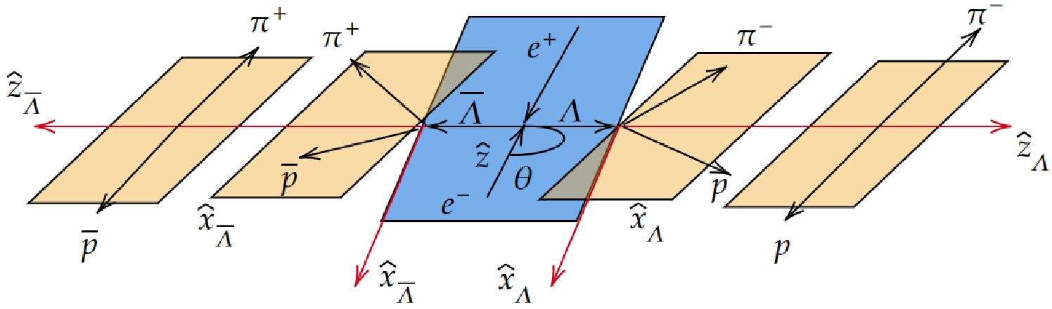
Figure 1. (color online) Definition of the coordinate system used to describe
$e^{+} e^{-} \rightarrow \Lambda\bar{\Lambda} \to p \bar{p}\pi^{+}\pi^{-}$ .The general expression for the joint density matrix of a
$ \Lambda\bar{\Lambda} $ pair is [27]$ \begin{equation} \rho_{\Lambda\bar{\Lambda}}=\sum\limits_{{\mu\upsilon}=0}^{3}{C}_{\mu\upsilon}\sigma_{\mu}^{\Lambda}\otimes\sigma_{\upsilon}^{\bar{\Lambda}}, \end{equation} $

(2) where a set of four Pauli matrices
$ \sigma_{\mu}^{\Lambda} $ ($ \sigma_{\upsilon}^{\bar{\Lambda}} $ ) in the Λ($ \bar{\Lambda} $ ) rest frame is used, and$ {C}_{\mu\upsilon} $ is a$ 4 \times 4 $ real matrix representing the polarization and spin correlations of the baryons. The elements of the$ {C}_{\mu\upsilon} $ matrix are functions of the production angle θ of the Λ baryon [28],$ \begin{equation} \begin{bmatrix} 1+\alpha_{\psi}\cos^{2}\theta &\gamma_{\psi}P_{e}\sin\theta& \beta_{\psi} \sin \theta \cos \theta &(1+\alpha_{\psi})P_{e}\cos \theta\\ \gamma_{\psi}P_{e}\sin\theta & \sin^{2} \theta & 0 &\gamma_{\psi}\sin \theta \cos \theta\\ - \beta_{\psi} \sin\theta \cos\theta& 0 &\alpha_{\psi}\sin^{2}\theta &-\beta_{\psi}P_{e}\sin\theta\\ -(1+\alpha_{\psi})P_{e}\cos\theta&-\gamma_{\psi}\sin \theta\cos\theta&-\beta_{\psi}P_{e}\sin\theta&-\alpha_{\psi}-\cos^{2}\theta \end{bmatrix}, \end{equation} $

(3) where
$ \beta_{\psi}=\sqrt{1-\alpha_{\psi}^{2}} \sin \Delta\Phi $ ,$ \gamma_{\psi}=\sqrt{1-\alpha_{\psi}^{2}} \cos \Delta \Phi $ ,$ \alpha_{\psi}^{2}+ \beta_{\psi}^{2}+ \gamma_{\psi}^{2}=1 $ , and$ P_{e} $ is the polarization of the electron beam. Two factors are naturally connected to the process of the ratio of two helicity amplitudes$ \alpha_{\psi} $ and the relative phase of the two helicity amplitudes$ \Delta\Phi $ in the real coefficients$ {C}_{\mu\upsilon} $ of Eq. (3). The joint angular distribution of the$ p/\bar{p} $ pair within the current formalism is described as follows [27]:$ \begin{align} {\rm T_{r}}\rho_{p\bar{p}}\propto\sum\limits_{{\mu\upsilon}=0}^{3}\alpha_{\mu}^{\Lambda}\alpha_{\upsilon}^{\bar{\Lambda}}, \end{align} $

(4) where
$ \alpha_{\mu}^{\Lambda}(\theta_{1},\; \varphi_{1},\; \alpha_{-}) $ and$ \alpha_{\upsilon}^{\bar{\Lambda}}(\theta_{2},\; \varphi_{2},\; \alpha_{+}) $ represent the correlations of the spin density matrices in the sequential decays, the full expressions for which can be found in [27], and$ \alpha_{-}(\alpha_{+}) $ are the decay parameters for$ \Lambda \rightarrow p \pi^{-} $ ($ \bar{\Lambda} \rightarrow \bar{p}\pi^{+} $ ). In the helicity frame of Λ,$ \theta_{1} $ and$ \varphi_{1} $ are the spherical coordinates of p relative to Λ. An event of the reaction$ J/\psi \rightarrow \Lambda\bar{\Lambda} \rightarrow p \bar{p}\pi^{+}\pi^{-} $ is specified by the five dimensional vector$ \xi=(\theta,\; \Omega_{1}(\theta_{1},\; \varphi_{1}),\; \Omega_{2}(\theta_{2},\; \varphi_{2})) $ , and the joint angular distribution$ \mathcal{W}(\xi) $ can be expressed as$ \begin{aligned}[b] \mathcal{W}(\xi)=& \mathcal{F}_{0}(\xi)+\sqrt{1-\alpha_{\psi}^{2}}\sin(\Delta\Phi)(\alpha_+\cdot\mathcal{F}_{3}-\alpha_-\cdot\mathcal{F}_{4}) \\ &+\alpha_-\alpha_+(\mathcal{F}_{1}+\sqrt{1-\alpha_{\psi}^{2}}\cos(\Delta\Phi)\cdot\mathcal{F}_{2}+\alpha_{\psi}\cdot\mathcal{F}_{5}) \\ & +\alpha_-\cdot\mathcal{F}_{6}+\alpha_+\cdot\mathcal{F}_{7}-\alpha_-\alpha_+\cdot\mathcal{F}_{8}, \end{aligned} $

(5) where the angular functions
$ \mathcal{F}_{i}(\xi) $ (i = 0, 1,..., 8) are defined as$ \begin{aligned} &\mathcal{F}_{0}(\xi)=1+\alpha_{\psi}\cos^{2}\theta,\\ &\mathcal{F}_{1}(\xi)=\sin^{2}\theta \sin\theta_{1}\cos\varphi_{1}\sin\theta_{2}\cos\varphi_{2}-\cos^{2}\theta\cos\theta_{1}\cos\theta_{2},\\ &\mathcal{F}_{2}(\xi)=\sin\theta \cos\theta(\sin\theta_{1}\cos\theta_{2}\cos\varphi_{1}-\cos\theta_{1}\sin\theta_{2}\cos\varphi_{2}),\\ &\mathcal{F}_{3}(\xi)=\sin\theta \cos\theta \sin\theta_{2}\sin\varphi_{2},\\ &\mathcal{F}_{4}(\xi)=\sin\theta \cos\theta \sin\theta_{1}\sin\varphi_{1},\\ &\mathcal{F}_{5}(\xi)=\sin^{2}\theta \sin\theta_{1}\sin\varphi_{1}\sin\theta_{2}\sin\varphi_{2}-\cos\theta_{1}\cos\theta_{2},\\ &\mathcal{F}_{6}(\xi)=P_{e}(\gamma_{\psi}\sin\theta \sin\theta_{1}\cos\varphi_{1}-(1+\alpha_{\psi})\cos\theta \cos\theta_{1}), \\ &\mathcal{F}_{7}(\xi)=P_{e}(\gamma_{\psi}\sin\theta \sin\theta_{2}\cos\varphi_{2}+(1+\alpha_{\psi})\cos\theta \cos\theta_{2}), \\ &\mathcal{F}_{8}(\xi)=P_{e}\beta_{\psi}\sin\theta(\cos\theta_{1}\sin\theta_{2}\sin\varphi_{2}+\sin\theta_{1}\sin\varphi_{1}\cos\theta_{2}). \end{aligned} $

(6) Eq. (5) contains four terms:
$ \mathcal{F}_{0} $ describes the angular distribution of Λ, and$ \mathcal{F}_{3} $ and$ \mathcal{F}_{4} $ account for the transverse polarization of Λ and$ \bar{\Lambda} $ , respectively. The spin correlations between the two hyperons are described by$ \mathcal{F}_{1} $ ,$ \mathcal{F}_{2} $ , and$ \mathcal{F}_{5} $ . The terms$ \mathcal{F}_{6} $ ,$ \mathcal{F}_{7} $ , and$ \mathcal{F}_{8} $ describe the beam polarization. In Eq. (5), the input values of$ \alpha_{-} $ ,$ \alpha_{+} $ ,$ \alpha_{\psi} $ , and$ \Delta\Phi $ are all from Ref. [18]. A study is conducted on the observable$ A_{CP} $ , which represents the magnitude of$ CP $ violation, under different polarization rates.$ A_{CP} $ is defined as$ A_{CP}=\frac{\alpha_{-}+\alpha_{+}}{\alpha_{-}-\alpha_{+}} $ . Using the maximum likelihood to fit the angular distribution of Eq. (5),$ \alpha_{-} $ and$ \alpha_{+} $ can be extracted and$ A_{CP} $ can be calculated. Experimentally, statistical error plays a dominant role in assessing the magnitude of$ CP $ violation. Hence, this study primarily investigates the statistical error associated with the magnitude of$ CP $ violation under different polarization rates.The Λ polarization vector
$ \mathbf{P_{\Lambda}} $ is defined in the rest frame of Λ, as shown in Ref. [28]:$ \begin{align} \mathbf{P_{\Lambda}}=\frac{\gamma_{\psi} P_{e}\sin\theta\hat{x}_{1}-\beta_{\psi} \sin\theta \cos\theta\hat{y}_{1}-(1+\alpha_{\psi})P_{e}\cos\theta\hat{z}_{1}}{1+\alpha_{\psi}\cos^{2}\theta}. \end{align} $

(7) The distribution of the module of
$ \left|\mathbf{P_{\Lambda}}\right| $ against the polar angle of Λ is determined, as shown in Fig. 2.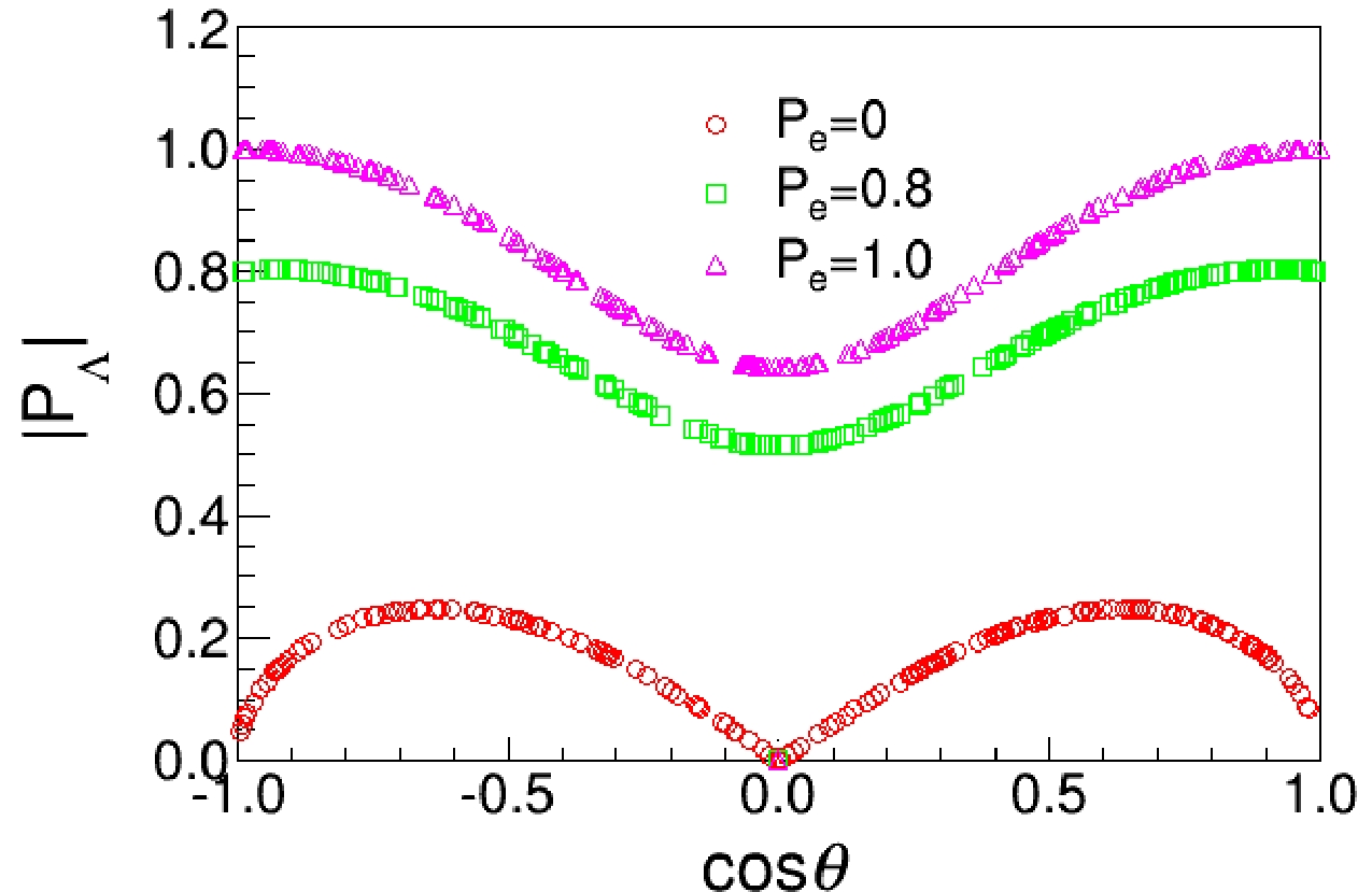
Figure 2. (color online) Distribution of
$\mathbf{P_{\Lambda}}$ against$\cos\theta$ . The red circles, green squares, and pink triangles represent the three cases of electron beam polarization 0, 0.8, and 1.0, respectively.The relationship between electron beam polarization and the polarization of Λ can be described by the following formula [28]:
$ \begin{aligned}[b] \left \langle \mathbf{P_{\Lambda}} \right \rangle=&\frac{(1-\alpha_{\psi}^{2})\sin^{2}(\Delta\Phi)}{\alpha_{\psi}^{2}(3+\alpha_{\psi})}\Bigg(3+2\alpha_{\psi}-3(1+\alpha_{\psi})\frac{\arctan\sqrt{\alpha_{\psi}}}{\sqrt{\alpha_{\psi}}}\Bigg)\\&+ \frac{3(1+\alpha_{\psi})^{2}}{\alpha_{\psi}(3+\alpha_{\psi})}\left(1-\frac{1-\alpha_{\psi}}{1+\alpha_{\psi}}\cos^{2}(\Delta\Phi)\frac{\arctan\sqrt{\alpha_{\psi}}}{\sqrt{\alpha_{\psi}}}\right)P^{2}_{e} . \end{aligned} $

(8) Figure 3 provides an intuitive representation of the relationship between the polarization of Λ and the polarization of the electron beam.

Figure 3. Relationship between the polarization of Λ and the polarization of the electron beam.
-
Charged tracks are selected based on the criteria in the fast simulation. Efficiency loss occurs owing to the acceptance requirement
$ |\cos\theta|\; < \; 0.93 $ , where θ is set in reference to the beam direction, and the requirements on the Λ mass and decay vertex. The decay process$ J/\psi \rightarrow \Lambda\bar{\Lambda} $ can be described as follows: Λ decays into a p and$ \pi^{-} $ , and$ \bar{\Lambda} $ decays into a$ \bar{p} $ and$ \pi^{+} $ . Therefore, the candidate event must have at least four charged tracks. Charged tracks are divided into two categories, where positively charged tracks are p and$ \pi^{+} $ , and negatively charged tracks are$ \bar{p} $ and$ \pi^{-} $ . Based on the momentum of the tracks, the momentum of the particle track can subsequently be identified as$ p (\bar{p}) $ or$ \pi^{+} (\pi^{-}) $ . Specifically, particles with a momentum exceeding 500 MeV/c are identified as$ p (\bar{p}) $ , whereas those with a momentum less than 500 MeV/c are classified as$ \pi^{+} (\pi^{-}) $ . For selected events, multiple charged tracks must be present for p,$ \bar{p} $ ,$ \pi^{+} $ , and$ \pi^{-} $ . A second vertex fit is performed by looping over all combinations of positive and negative charged tracks. The p($ \bar{p} $ )$ \pi^{-} $ ($ \pi^{+} $ ) pairs selected must decay from the same vertex. The invariant mass of Λ($ \bar{\Lambda} $ ) must fall within the range$ 1.1107<M_{p \pi^{+}}<1.1207 $ GeV/$ c^{2} $ ($ 1.1107< M_{\bar{p} \pi^{-}}<1.1207 $ GeV/$ c^{2} $ ). Figure 4 shows the spectrum of the energy invariant mass of p and$ \pi^{-} $ from Λ in the mass frame after applying the aforementioned selection criteria, corresponding to approximately 3.5 times the mass resolution of Λ. The event selection efficiency is finally determined to be 38.2%. The influence of the polarization of the electron beam on event selection efficiency is also studied, and the selection efficiency is found to be unaffected by beam polarization.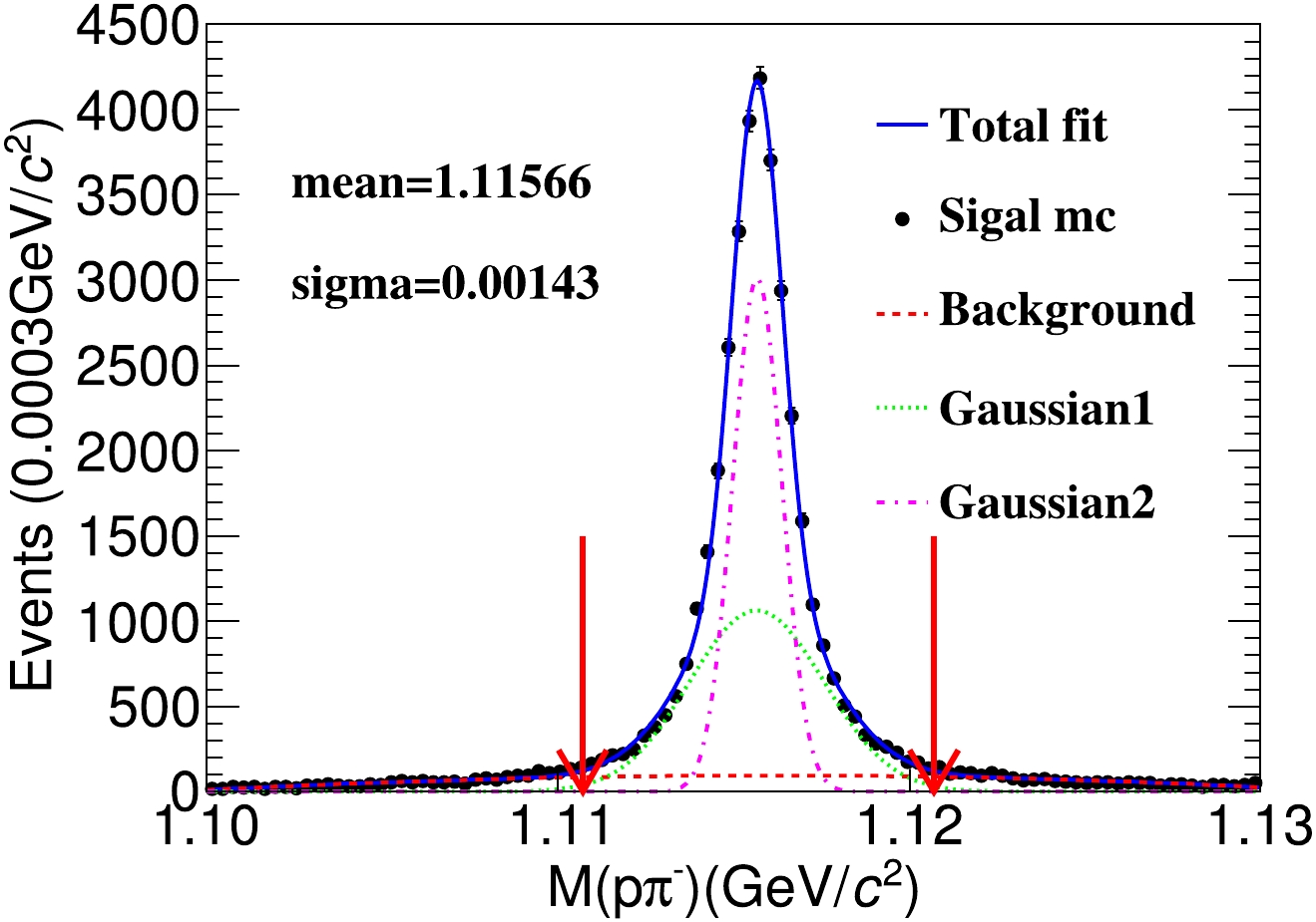
Figure 4. (color online) Spectrum of the invariant mass of p and
$\pi^{-}$ in the mass frame of Λ. The black dots with error bars represent the signal MC sample. The blue solid curve represents the fit results, where the signal function is a double Gaussian consisting of a pink dashed line and green dashed line. The background is represented by the solid red line, which is modeled using a second-order polynomial. -
To enhance the performance of the detector, the momentum resolution and selection efficiency of the charged tracks can be further optimized with the help of the fast simulation software. The optimization results are presented below.
● Tracking efficiency
The detector is capable of identifying the following charged particles in the final state: electrons, muons, pions, kaons, and protons. A wide momentum range must be covered while maintaining a high reconstruction efficiency throughout this range. To further enhance the capability of reconstructing low-momentum tracks, different materials or sophisticated tracking algorithms can be employed to further enhance the capability of low momentum track reconstruction in the design portion of the STCF tracking system. The low momentum final-state particles π mesons are produced by the decay
$ J/\psi \rightarrow \Lambda\bar{\Lambda} \rightarrow p \bar{p}\pi^{+}\pi^{-} $ , which is a useful option for enhancing the resolution of low momentum particles and optimizing detector response. In this analysis, the tracking efficiency scaling factor is gradually increased from 1.0 to 2.0. The scale factor represents the ratio of the efficiency. Figure 5 shows that the final selection efficiency greatly improves between 1.0 and 1.1, resulting in an improvement from 38.2% to 43.7%.
Figure 5. (color online) Scales of charged track efficiency against selection efficiency.
● Momentum resolution of tracking
In the fast simulation, the momentum resolution of the charged track can also be adjusted for improvement. The resolutions of the tracking system in the
$ xy $ plane and z direction are$ \sigma_{xy} $ and$ \sigma_{z} $ , respectively. The default values of$ \sigma_{xy} $ and$ \sigma_{z} $ are 130 μm and 2480 μm, respectively. Optimization is performed on$ \sigma_{xy} $ from 0 to 130 μm, and on$ \sigma_{z} $ from 0 to 2480 μm, resulting in no significant change in detection efficiency, as demonstrated in Fig. 6.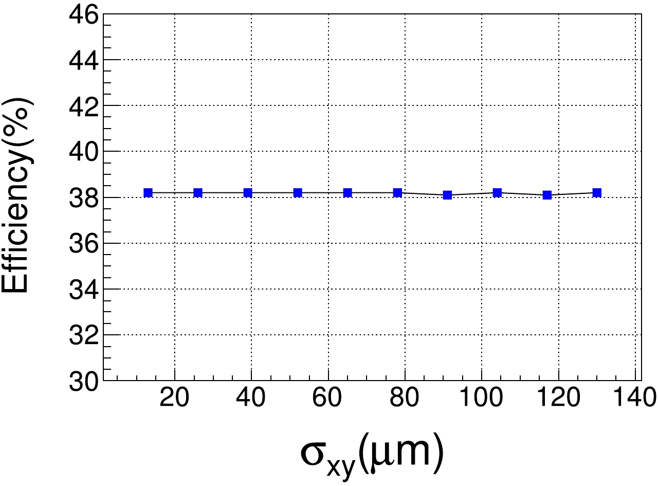
Figure 6. (color online) Momentum resolution of charged tracks against selection efficiency.
-
Based on the joint angular distribution, a maximum likelihood fit is performed with four free parameters (
$ \alpha_{\psi} $ ,$ \alpha_{-} $ ,$ \alpha_{+} $ , and$ \Delta\Phi $ ). The joint likelihood function, as defined in Ref. [29] and shown in Eq. (9), is used for this purpose.$ \begin{aligned}[b] \mathcal{L}=&\prod\limits_{i=1}^{N}\mathcal{P}(\xi^{i}, \alpha_{\psi}, \alpha_-, \alpha_+, \Delta\Phi)\\=&\prod\limits_{i=1}^{N}\mathcal{C}\mathcal{W}(\xi^{i}, \alpha_{\psi},\alpha_-, \alpha_+, \Delta\Phi)\epsilon(\xi^{i}), \end{aligned} $

(9) The probability density function of the kinematic variable
$ \xi^{i} $ for event i, denoted as$ \mathcal{P}(\xi^{i},\; \alpha_{\psi},\; \alpha_{-},\; \alpha_{+},\; \Delta\Phi) $ , is used in the maximum likelihood fit. The fit is performed using Eq. (6), where$ \mathcal{W}(\xi^{i},\; \alpha_{\psi},\; \alpha_{-},\; \alpha_{+},\; \Delta\Phi) $ represents the weights assigned to each event. The detection efficiency is represented by$ \epsilon(\xi^{i}) $ , and N denotes the total number of events. The normalization factor, denoted as$\mathcal{C}^{-1} =\frac{1}{N_{\rm MC}}\sum\limits^{N_{\rm MC}}_{j=1}\mathcal{W}(\xi^{j},\; \alpha_{\psi},\; \alpha_{-}, \; \alpha_{+},\; \Delta\Phi)\epsilon(\xi^{j})$ , estimates the$ N_{\rm MC} $ events generated with the phase space model, which is approximately ten times the size of mDIY MC. Usually, the minimization of$ -{\rm ln}\mathcal{L} $ is performed using MINUIT [30]:$ \begin{align} -{\rm ln}\mathcal{L}=-\sum\limits^{N}_{i=1}{\rm ln}\mathcal{C}\mathcal{W}(\xi^{i},\alpha_{\psi},\alpha_-,\alpha_+,\Delta\Phi)\epsilon(\xi^{i}) . \end{align} $

(10) In this analysis, we extrapolate the sensitivity of
$ CP $ violation for a large number of$ J/\psi $ events generated at the future STCF, considering the effects of excessive disk pressure. This extrapolation is based on the relationship between the sensitivity of$ CP $ violation and the generated 0.1 trillion$ J/\psi $ events. We investigate this relationship using a sample size ranging from 0.01 to 0.1 trillion$ J/\psi $ , with a step size of 0.01 trillion$ J/\psi $ . The sensitivity analysis is presented in Fig. 7, where we examine the impact of event statistics on the sensitivity of$ CP $ violation. The sensitivity can be described using the following formula: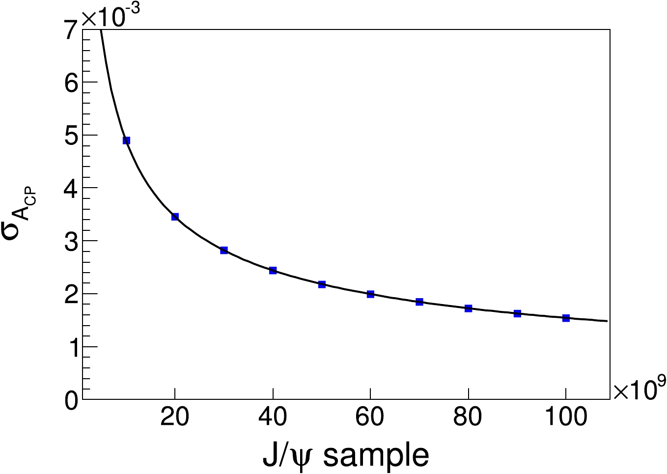
Figure 7. (color online) Blue dots represent the statistical errors on
$CP$ violation, and the black line is fit using Eq. (11).$ \begin{equation} \sigma_{A_{CP}}\times\sqrt{N_{\rm fin}}=k. \end{equation} $

(11) The variable
$N_{\rm fin}$ represents the number of events that pass the final selection criteria, and k is a constant with a value of 7.82.As shown in Fig. 7, the sensitivity of statistical errors increases proportionally with the square root of the number of signal events. This observation provides a foundation for extrapolating
$ CP $ violation sensitivity from the size of the data sample.Five different beam polarizations are utilized to generate a sample of 0.1 trillion MC events, with the specific aim of investigating the quantity
$ \sigma_{A_{CP}} $ . The resulting five sets of data points are fit using Eq. (12) [28]:$ \begin{equation} \sigma_{A_{CP}}\approx \sqrt{\frac{3}{2}} \frac{1}{\alpha_-\sqrt{N_{\rm sig}}\sqrt{\left \langle P_{\Lambda}^{2} \right \rangle}}. \end{equation} $

(12) Under the same sample size, the obtained results align with those in Ref. [31], maintaining consistency at the order of magnitude level. By extrapolating the number of
$ J/\psi $ events based on the 3.4 trillion events expected to be generated annually by the future STCF, as demonstrated in Figs. 7 and 8, it is apparent that the statistical sensitivity of$ CP $ violation will reach the order of$ \mathcal O (10^{-5}) $ at a beam polarization of 80%.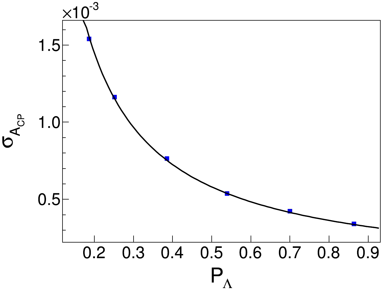
Figure 8. (color online) Blue dots represent the values of
$\sigma_{A_{CP}}$ under different Λ polarizations. -
In this study, the detection efficiency and
$ CP $ violation sensitivity of the$ J/\psi \rightarrow \Lambda\bar{\Lambda} \rightarrow p \bar{p}\pi^{+}\pi^{-} $ process under different beam polarizations are investigated using$ 1.89 \times 10^8 J/\psi \rightarrow \Lambda \bar{\Lambda} $ MC samples generated by the fast simulation package developed during the pre-research stage of the STCF. We find that the polarization of the electron beam does not affect the final detection efficiency; however, the sensitivity of$ CP $ violation increases with increasing electron beam polarization. Moreover, if the tracking efficiency of charged particles with low momentum can be improved by 10% compared to the baseline in the fast simulation, the final detection efficiency will significantly improve by 14.3%. This places high demands on each sub-detector in the expected STCF design. If the future STCF can achieve significant luminosity improvement and beam polarization, the sensitivity of$ CP $ violation will be greatly enhanced, making it an ideal place to test$ CP $ violation in the SM. -
We thank the Hefei Comprehensive National Science Center for their strong support with the STCF key technology research project.
Prospects of CP violation in Λ decay with a polarized electron beam at the STCF
- Received Date: 2023-06-28
- Available Online: 2023-11-15
Abstract: Based on


 DownLoad: