


 Abstract
 HTML
HTML Reference
 Related
 PDF
PDF


-
In the QCD phase diagram in the plane of the temperature and baryon chemical potential, it is conjectured that there is a critical end point (CEP) connecting the first-order phase transition line at a high baryon chemical potential and the continuous crossover in the high temperature regime [1, 2], as presented in [3−5] with related reviews. Because of the importance of CEP in the studies of the QCD phase structure, that would deepen our understanding of the fundamental properties of strongly correlated QCD matter in extreme conditions, recent years have seen significant progress in the studies of CEP from both the theoretical and experimental aspects.
Lattice QCD simulations indicate that there is no CEP in the region of
$ \mu_B/T\lesssim 2 \sim 3 $ [6], where$ \mu_B $ denotes the baryon chemical potential and T is the temperature. Reliable computations of the lattice QCD at larger$ \mu_B $ are hindered by the rapidly increasing severity of the sign problem at finite chemical potential [7−9]. The region of reliable calculations can be further extended to that of$ \mu_B/T\sim 4 $ within the functional continuous field approaches; for instance, the functional renormalization group (fRG) [5, 10−12] and Dyson-Schwinger equations [4], which should have passed through benchmark tests of the lattice QCD in the small$ \mu_B $ regime. It is interesting to note that recent first-principles functional approaches have exhibited a convergent estimate of the location of CEP in the phase diagram at a small region at approximately$ \mu_B \sim 600 $ MeV [13−15].The QCD critical end point is a second-order phase transition point, that belongs to the
$ Z(2) $ symmetry, i.e., Ising-like, universality class. Generally, fluctuation measurements, in particular, high-order non-Gaussian fluctuations, are sensitive to the critical behavior of the second-order phase transition. Thus, it has been proposed for a long time that one can use the fluctuations of conserved charges, such as the baryon number fluctuations, to search for the CEP [16−19]. Relevant experiments have been underway at the Relativistic Heavy Ion Collider (RHIC) over the last decade, and fluctuations of the proton, electric charge, and net-kaon numbers have been measured [20−29]. Remarkably, a non-monotonic dependence of the kurtosis of the net-proton distributions, i.e., the fourth-order proton number fluctuations, on the collision energy is observed with$ 3.1\, \sigma $ significance [25]. Although this observation does not yet provide evidence for the existence of a CEP in the QCD phase diagram [30, 31], it is indeed significant progress in this direction.The critical behavior of a phase transition is encoded in the cumulants of the net-proton or net-baryon number distributions, and hence these properties should also be reflected directly in the distribution function. In comparison with the cumulants, more information is included in the baryon number distributions, rather than a few moments of the distribution function. Moreover, the baryon number distributions can be used in some transport models of heavy-ion collisions [32, 33]. Therefore, it is interesting and useful to evaluate the baryon number distributions directly.
The baryon number distribution can be computed directly through the calculation of the canonical partition function [34]. However, the calculation becomes increasingly difficult with the increase of the baryon chemical potential, and it is almost inaccessible for the chemical freeze-out baryon chemical potentials in the Beam Energy Scan experiments at RHIC. In this work, we would like to adopt an alternative approach, and use a few order cumulants to reconstruct the baryon number distributions. This task is a typical inverse problem, that is ill-defined. Thanks to the rapid progress in statistics and computing science, a number of methods have been developed to deal with inverse problems. In this work, we choose two of them: the maximum entropy method (MEM) and the Gaussian process regression (GPR), which is abbreviated as the Gaussian process (GP), to reconstruct the baryon number distributions from a finite number of cumulants. Eventually, We would like to apply the reconstruction to cumulants, which are obtained in both theoretical calculations and experimental measurements.
This paper is organized as follows: In Sec. II we present a brief introduction of the relation between the baryon number distribution and the generalized baryon number susceptibilities. The approaches of the MEM and GP are discussed in Sec. III and Sec. IV, respectively. In Sec. V numerical setups for these two approaches are presented. In Sec. VI we use the two methods to reconstruct the baryon number distributions across the chiral phase transition and those at the collision energy
$\sqrt{s_{NN}}=$ 7.7 GeV. Finally, the conclusions and summary are presented in Sec. VII. -
We proceed with the basic relation between fluctuations and the probability distribution for a conserved charge, e.g., the net baryon number
$ N_{B} $ . The n-th order central moment of a net baryon number distribution is defined as$ \langle(\delta N_{B})^{n}\rangle= \sum\limits_{N_{B}=-\infty}^{\infty}(\delta N_{B})^{n}P(N_{B})\, , $

(1) with
$ \delta N_{B}\equiv N_{B}-\langle N_{B} \rangle $ , where$ P(N_{B}) $ denotes the probability distribution of the net baryon number$ N_{B} $ , and$ \langle N_{B} \rangle $ is its mean value. Consequently, if the probability distribution is known, one can readily obtain the relevant cumulants of different orders [34−36].For a system of a grand canonical ensemble in thermal equilibrium, the distribution cumulants of a conserved charge can be directly obtained by differentiating the thermodynamic potential of the system w.r.t. the chemical potential conjugate to the charge. Thus, the cumulants of the baryon number are provided by the generalized susceptibilities related to the baryon chemical potential
$ \mu_{B} $ , which is$ \chi_{n}^{B}=\frac{\partial^{n}}{\partial(\mu_{B}/T)^{n}}\frac{p}{T^{4}}\, , $

(2) with pressure p and temperature T, where the temperature is fixed. The pressure is directly related to the thermodynamic potential density as
$ p=-\Omega[T, \mu_{B}]\, . $

(3) The pressure as well as the thermodynamic potential of the QCD matter for a grand canonical ensemble in thermal equilibrium can be computed from lattice QCD simulations [7−9] and functional approaches, such as the fRG [5, 11, 13] and Dyson-Schwinger equations [4]. In the fRG approach, the thermodynamic potential is extracted from the difference between the effective action at finite T and
$ \mu_B $ and that in the vacuum, that is,$ \Omega[T, \mu_{B}]=\frac{T}{V}\Big{(}\Gamma[\bar{\Phi}]\Big{|}_{T, \mu_{B}}-\Gamma[\bar{\Phi}]\Big{|}_{T=\mu_{B}=0}\Big{)}\, , $

(4) with volume V, where Γ is the effective action, and
$ \bar{\Phi} $ denotes a collection of different fields on their respective equations of motion [31, 37, 38].For the lowest four orders, the generalized susceptibilities of the baryon number
$ \chi_{n}^{B} $ in Eq. (2) are related to the cumulants in Eq. (1) through equations as follows,$ \chi_{1}^{B}=\frac{1}{VT^{3}}\langle N_{B} \rangle\, , \tag{5a}$

$ \chi_{2}^{B}=\frac{1}{VT^{3}}\langle (\delta N_{B})^{2} \rangle\, , \tag{5b}$

$ \chi_{3}^{B}=\frac{1}{VT^{3}}\langle (\delta N_{B})^{3} \rangle\, , \tag{5c}$

$ \chi_{4}^{B}=\frac{1}{VT^{3}}\Big{(}\langle (\delta N_{B})^{4}\rangle-3\langle(\delta N_{B})^{2}\rangle^{2}\Big{)}\, . \tag{5d} $

It is also convenient to use the cumulants directly related to
$ \chi_{n}^{B} $ , given by$ \kappa_{n}=(VT^{3})\chi_{n}^{B}\, , $

(6) which are proportional to the volume V, and thus are extensive. In the following, we will use the cumulants calculated in thermodynamics from Eq. (2), and attempt to reconstruct the baryon number distributions in Eq. (1) by employing the MEM and GP.
-
In this section, we present the distribution reconstruction with the maximum entropy strategy. The maximum entropy method embedded in the Bayesian inference has been successfully applied to ill-posed inverse problems for over 30 years [39−42]. It is straightforward to apply the MEM to the reconstruction of the net baryon number distributions, based on several lowest-order cumulants of the distribution.
We begin with a rather general discussion. Suppose there are some known data of n-th order cumulants
$ \kappa=(\kappa_1, \kappa_2, \cdots, \kappa_n, \cdots) $ and some prior information I (e.g. the distribution is positive definite), the probability of the distribution of$ P(N_{B}) $ with the previous conditions is denoted as$ \mathscr{P}[P|\kappa, I] $ , that is also referred to as the posterior probability. We are then are left with the task to determine a proper distribution$ P(N_{B}) $ , such that the resulting posterior probability$ \mathscr{P}[P|\kappa, I] $ reaches its maximum value. The Bayesian theorem states that one can access this probability from the likelihood probability and the prior probability as follows$ \mathscr{P}[P|\kappa, I]=\frac{\mathscr{P}[\kappa|P, I]\mathscr{P}[P|I]}{\mathscr{P}[\kappa|I]}\, , $

(7) where
$ \mathscr{P}[\kappa|P, I] $ refers to the likelihood probability, which describes the observed data distributions and$ \mathscr{P}[P|I] $ is the so-called prior probability, which is a prior estimate of$ P(N_{B}) $ without any observed data. The denominator on the right side of Eq. (7),$ \mathscr{P}[\kappa|I] $ , is a normalization constant that can be safely ignored in the inference process in what follows. The observed data distributions are most commonly assumed to be Gaussian-like, i.e.,$ \mathscr{P}[\kappa|P, I]\propto \;{\rm{e}}^{-L}\, , $

(8) with
$ L=\frac{1}{2}\sum\limits_{i, j}(\kappa_i-\kappa^{P}_i)C^{-1}_{ij}(\kappa_j-\kappa^{P}_j)\, , $

(9) where
$ \kappa_i $ indicates an average of the i-th order cumulant from the observed data and$ \kappa^{P}_i $ with a superscript P that is calculated from the distribution$ P(N_{B}) $ .$ C_{ij} $ is the covariance matrix for the observed data. If only the likelihood probability in Eq. (8) is maximized, it would be equivalent to the$ \chi^2 $ -fitting. Unfortunately, for this ill-posed problem, the number of data of cumulants in the order of$ {\cal{O}}(1) $ , is considerably smaller than that of the baryon number distributions$ P(N_{B}) $ in the order of$ {\cal{O}}(100) $ that we would like to reconstruct, which could result in a plethora of spurious solutions for the$ \chi^2 $ -fitting. The prior probability then plays the role as a penalty term. In the context of MEM, the prior probability reads$ \mathscr{P}[P|I]\propto \;{\rm{e}}^{\alpha S(P)}\, , $

(10) where S is the entropy of the baryon number distribution
$ P(N_{B}) $ . For a discrete probability distribution, we adopt the Shannon entropy as follows$ S=-\sum\limits_{i=-\infty}^{\infty}P_i\ln(P_i)\, , $

(11) where we have used the shorthand notation
$ P_i\equiv P(N_{B}) $ . The hyperparameter α in Eq. (10) is used to control the relative weight between the likelihood probability and prior probability. Finally, we are led to the posterior probability that is expressed as$ \mathscr{P}[P|\kappa, I]\propto \;{\rm{e}}^{Q(P)}\, , \qquad Q(P)=\alpha S-L\, , $

(12) and thus, one is required to maximize the function
$ Q(P) $ . Because$ Q(P) $ is a concave functional of P, it is possible to use, e.g., convex optimization techniques, to maximize it.If the errors of cumulants calculated from the generalized susceptibilities of the baryon number in Eq. (2) are neglected, that is, the covariance matrix in Eq. (9) approaching the limit
$ C\to 0 $ , the likelihood probability, i.e., the L part in Eq. (12), can be reduced to a few constraints, which is expressed as$ \kappa_n=\kappa_n^{P}=\sum\limits_{i}K_{ni}P_i\, , $

(13) where
$ K_{ni} $ indicates the kernel of cumulant$ \kappa_n $ . Specifically, if$ K_{n=0i}=1 $ is chosen, Eq. (13) leaves us with$ \kappa_0=1 $ , that is, the normalization for the distribution function. Considering the constraints discussed above, the entropy in Eq. (11) is extended to the equation as follows$ S=-\sum\limits_{i=-\infty}^{\infty}P_i\ln(P_i)+\sum\limits_{n=0}^{n_{{\rm{trunc}}}}\lambda_n\left(\sum\limits_{i=-\infty}^{\infty} K_{ni}P_i-\kappa_n\right)\, , $

(14) where
$ \lambda_n $ is the Lagrange multiplier for each constraint, and$ n_{{\rm{trunc}}} $ stands for the maximal order of cumulants used to reconstruct the distribution. Maximizing Eq. (14) with respect to the probability distribution$ P_i $ and the multipliers$ \lambda_n $ , one is led to an analytic baryon number distribution, which reads$ P_i=\exp\left(\sum\limits_{n=1}^{n_{{\rm{trunc}}}}\lambda_n K_{ni}+\lambda_0-1\right)\, , $

(15) where the Lagrange multipliers are determined by the constraints in Eq. (13).
-
The Gaussian process regression is a powerful method to infer the probability function from a finite number of observations, cf. reviews [43, 44], paper[45], and textbooks [46]. Recently, it has been employed in the study of parton distribution functions from lattice QCD [47−49] and the reconstruction of the QCD spectral functions from fRG [50−52]. In this section, the discrete GP, which is suitably applied to the net baryon number distribution, is introduced.
Generally, the probability distribution of the baryon number distribution can be described by a discrete Gaussian process,
$ P(N_{B})\sim {\cal{GP}}\Big(\mu(N_{B}), C(N_{B}, N^{\prime}_{B})\Big)\, , $

(16) with the mean function
$ \mu(N_{B}) $ and the covariance function or covariance matrix$ C(N_{B}, N^{\prime}_{B}) $ , that is symmetric, i.e.,$ C(N_{B}, N^{\prime}_{B})=C(N^{\prime}_{B}, N_{B}) $ . For the GP, the probability of the function is described by a multivariate Gaussian or normal distribution, which includes a finite set of sample points$ \{N_{B_{1}}, N_{B_{2}}, ..., N_{B_{n}}\} $ , that is,$ \begin{align} \left(\begin{array}{c} P(N_{B_{1}}) \\ \vdots \\ P(N_{B_{n}}) \end{array}\right) & \sim {\cal{N}}\left(\left(\begin{array}{c} \mu(N_{B_{1}}) \\ \vdots \\ \mu(N_{B_{n}}) \end{array}\right), \right.\\ &\left.\left(\begin{array}{ccc} C(N_{B_{1}}, N_{B_{1}}) & \ldots & C(N_{B_{1}}, N_{B_{n}}) \\ \vdots & \ddots & \vdots \\ C(N_{B_{n}}, N_{B_{1}}) & \ldots & C(N_{B_{n}}, N_{B_{n}}) \end{array}\right)\right) \, , \end{align} $

(17) where
$ {\cal{N}} $ stands for the n-dimensional normal distribution. In particular, this approach is constructed from a complete family of functions, such that there is no restriction on the functional basis or no artificial truncation.For the reconstruction of baryon number distributions, it is necessary to add a set of observations, here denoted by
$ O_i $ , to Eq. (14), which yields$ \begin{align} \left(\begin{array}{c} P(N_{B}) \\ {\boldsymbol{O}} \end{array}\right) &\sim {\cal{N}}\Bigg(\left(\begin{array}{c} \mu(N_{B}) \\ {\boldsymbol{\mu}}_{O} \end{array}\right), \\ &\left(\begin{array}{cc} C\left(N_{B}, N_{B}^{\prime}\right) & {\boldsymbol{C}}^\top(N_{B}) \\ {\boldsymbol{C}}\left(N^{\prime}_{B}\right) & {\boldsymbol{C}}+\sigma_n^2 \cdot {\bf{1}} \end{array}\right)\Bigg)\, , \end{align} $

(18) with
$ {{\boldsymbol{\mu}}_{O}}_i \equiv\mu(O_i)\, , \qquad {\boldsymbol{C}}_i(N_{B})\equiv C(O_i, N_{B})\, , $

(19) $ {\boldsymbol{C}}_{ij} \equiv C(O_i, O_j)\, . $

(20) where
$ \sigma_n^2 $ denotes the pointwise variance due to the measurement noise in the observations. Notably, the observation can either be the baryon number distribution$ P(N_{B}) $ at some values of$ N_{B} $ , or the cumulants of the distribution as shown in Eq. (13). Thus, given the posterior information on baryon number distributions provided by the observations$ O_i $ , one is led to the conditional probability of baryon number distributions [46], as follows$ P(N_{B}) \big | {\boldsymbol{O}} \sim{\cal{N}}\Big(\bar\mu(N_{B}), \bar C(N_{B}, N_{B}^{\prime})\Big)\, , $

(21) with
$ \begin{align}[b] &\bar\mu(N_{B}) \\ \equiv &\mu(N_{B})+{\boldsymbol{C}}^{\top}(N_{B})\Big({\boldsymbol{C}}+\sigma_n^2 \cdot {\bf{1}}\Big)^{-1}({\boldsymbol{O}}-{\boldsymbol{\mu}}_{O})\, , \end{align} $

(22) $ \begin{align}[b] &\bar C(N_{B}, N_{B}^{\prime})\\ \equiv&C(N_{B}, N_{B}^{\prime})-{\boldsymbol{C}}^{\top}(N_{B})\Big({\boldsymbol{C}}+\sigma_n^2 \cdot {\bf{1}}\Big)^{-1} {\boldsymbol{C}}(N_{B}^{\prime}) \, , \end{align} $

(23) which follow from the standard results of multivariate normal distribution. However, the probability of the observed data also obeys the multivariate normal distribution, which is
$ {\boldsymbol{O}}_i \sim {\cal{N}}\Big({{\boldsymbol{\mu}}_{O}}_i, {\boldsymbol{C}}_{ij}\Big)\, , $

(24) with the mean value in Eq. (19) and the covariance in Eq. (20) given by
$ {{\boldsymbol{\mu}}_{O}}_i =\sum\limits_{N_{B}} K_{i}(N_{B})\, \mu(N_{B})\, , $

(25) $ {\boldsymbol{C}}_{ij}= \sum\limits_{N_{B}, N'_{B}} K_{i}(N_{B}) C(N_{B}, N_{B}^{\prime})K_{j}(N'_{B})\, , $

(26) where
$ K_{i}(N_{B}) $ corresponds to the kernel in Eq. (13) if the cumulants are observed. In the same way, the following is obtained$ {\boldsymbol{C}}_i(N_{B})=\sum\limits_{N_{B}^{\prime}} K_{i}(N'_{B}) C(N'_{B}, N_{B})\, . $

(27) Inserting Eq. (25), Eq. (26), and Eq. (27) into Eq. (22) and Eq. (23), we obtain
$ \begin{aligned}[b] \bar\mu(N_{B})= &\mu(N_{B})+\sum\limits_{i, j}\sum\limits_{N_{B}^{\prime}} K_{i}(N'_{B}) C(N'_{B}, N_{B})\\ & \times\Big({\boldsymbol{C}}+\sigma_n^2 \cdot {\bf{1}}\Big)^{-1}_{ij}({\boldsymbol{O}}_j-{{\boldsymbol{\mu}}_{O}}_j)\, , \end{aligned} $

(28) $ \begin{aligned}[b] \bar C(N_{B}, N_{B}^{\prime})=&C(N_{B}, N_{B}^{\prime})-\sum\limits_{i, j}\sum\limits_{N''_{B}N'''_{B}} K_{i}(N''_{B}) C(N''_{B}, N_{B})\\ & \times\Big({\boldsymbol{C}}+\sigma_n^2 \cdot {\bf{1}}\Big)^{-1}_{ij} K_{j}(N'''_{B}) C(N'''_{B}, N'_{B}) \, , \end{aligned} $

(29) where the summation over the subscripts
$ i, j $ applies for all observed data.In this work, we adopt the commonly used kernel function called the radial basis function (RBF), which reads
$ C(N_{B}, N'_{B})=\sigma_c^2 \exp \bigg(-\frac{(N_{B}-N'_{B})^2}{2 l^2}\bigg)\, , $

(30) where two hyperparameters denoted by
$ {\boldsymbol{\alpha}}=\{\sigma_c, l\} $ have been introduced, which are determined by minimizing the negative logarithm likelihood (NLL) probability in Eq. (24), to wit,$ \begin{aligned}[b] -\log\mathscr{P}[{\boldsymbol{O}};{\boldsymbol{\alpha}}]=&\frac{1}{2}({\boldsymbol{O}}-{\boldsymbol{\mu}}_{O})^{\top}\Big({\boldsymbol{C}}_{{\boldsymbol{\alpha}}}+\sigma_n^2 \cdot {\bf{1}}\Big)^{-1}({\boldsymbol{O}}-{\boldsymbol{\mu}}_{O})\\ &+\frac{1}{2}\log\det\Big({\boldsymbol{C}}_{{\boldsymbol{\alpha}}}+\sigma_n^2 \cdot {\bf{1}}\Big)+\frac{N}{2}\log(2\pi)\, , \end{aligned} $

(31) where the explicit dependence on the hyperparameters is shown, and N is the number of the observations.
-
In this section, we use a concrete example to illustrate how the baryon number distribution is reconstructed based on a few first low-order cumulants, using the MEM and GP. Here, we use the first four-order cumulants of baryon number distributions obtained in fRG through Eq. (2) at temperature
$ T=130 $ MeV and the baryon chemical potential$ \mu_B=406 $ MeV [31]. The volume in Eq. (6) is chosen as$V=542~ {\rm{fm}}^3$ , and the resulting values for the first four-order cumulants are presented in the line of fRG input in Table 1.$ \kappa_1 $ 

$ \kappa_2 $ 

$ \kappa_3 $ 

$ \kappa_4 $ 

$ \lambda_0 $ 

$ \lambda_1 $ 

$ \lambda_2 $ 

$ \lambda_3 $ 

$ \lambda_4 $ 

fRG input 28.74 31.46 37.54 54.60 — — — — — MEM ( $ \kappa_1 $ ,

$ \kappa_2 $ input)

28.74 31.46 $ \sim 0^* $ 

$ \sim 0^* $ 

$ -1.643 $ 

$ \sim 0 $ 

$ -1.589 \times 10^{-2} $ 

— — MEM ( $ \kappa_1 $ ,

$ \kappa_2 $ ,

$ \kappa_3 $ input)

28.74 31.46 37.54 $ {1.099\times 10^4 }^* $ 

$ -1.526 $ 

$ -4.033\times 10^{-3} $ 

$ -1.595\times 10^{-2} $ 

$ 4.276\times 10^{-5} $ 

— MEM ( $ \kappa_1 $ ,

$ \kappa_2 $ ,

$ \kappa_3 $ ,

$ \kappa_4 $ input)

28.74 31.46 37.54 54.60 $ -1.086 $ 

$ -1.978\times 10^{-2} $ 

$ -1.567\times 10^{-2} $ 

$ 2.147\times 10^{-4} $ 

$ -3.182\times 10^{-6} $ 

GP ( $ \kappa_1 $ ,

$ \kappa_2 $ ,

$ \kappa_3 $ ,

$ \kappa_4 $ input)

28.74 31.46 37.33 54.75 — — — — — Table 1. Reconstruction of the baryon number distributions from several low-order cumulants obtained in fRG [31] within the MEM and GP. Numbers with a star are calculated with the reconstructed distribution. Values of the Lagrange multiples in Eq. (15) in the MEM are presented. See text for details.
For the MEM, we employ three different inputs to reconstruct the baryon number distribution. One is to use just the first two cumulants
$ \kappa_1 $ ,$ \kappa_2 $ as inputs; the next one adds$ \kappa_3 $ into the inputs; the last one adds$ \kappa_4 $ . The resulting baryon number distributions for the three different inputs are presented in Fig. 1. It is clearly observed that the difference arises in the tails of the distribution, i.e., the region far away from the mean value, when more information of high-order cumulants is encoded. In Table 1, we also present$ \kappa_3 $ and$ \kappa_4 $ of the baryon number distribution reconstructed from$ \kappa_1 $ and$ \kappa_2 $ , indicated by a star, and$ \kappa_4 $ from$ \kappa_1 $ ,$ \kappa_2 $ and$ \kappa_3 $ . It can be observed that the baryon number distribution reconstructed from$ \kappa_1 $ and$ \kappa_2 $ within the MEM is consistent with a discretized Gaussian distribution, that is,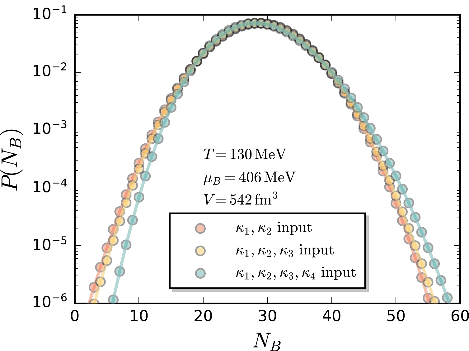
Figure 1. (color online) Baryon number distributions reconstructed from the cumulants obtained in fRG [31] with
$ T=130 $ MeV,$ \mu_B=406 $ MeV, and$V=542~ {\rm{fm}}^3$ by means of the MEM. Three different inputs are employed, corresponding to the input of only$ \kappa_1 $ and$ \kappa_2 $ , that of$ \kappa_1 $ through$ \kappa_3 $ , and that of$ \kappa_1 $ through$ \kappa_4 $ , respectively.$ P(N_B)\sim \exp\left({-\frac{(N_B-\kappa_ 1)^2}{2\kappa_2}}\right)\, , $

(32) and the non-Gaussian cumulants
$ \kappa_3 $ and$ \kappa_4 $ are very close to zero. The baryon number distribution reconstructed with$ \kappa_1 $ ,$ \kappa_2 $ and$ \kappa_3 $ , however, gives rise to a very large nonvanishing$ \kappa_4 $ as illustrated in Table 1. More detailed studies indicate that it is an artifact, that always occurs when cumulants of the odd number are used to reconstruct the distribution with the MEM. Moreover, values of the Lagrange multipliers in Eq. (15) for each reconstruction are presented in Table 1.For the reconstruction of baryon number distributions by the GP, it is necessary to provide more observations besides the cumulants. For instance, it is natural to assume that the baryon number distribution is non-negative, i.e.,
$ P(N_{B})\geq 0 $ for each value of$ N_{B} $ ; however, this property sometimes is violated in the reconstructed distribution by the GP, if only the cumulants are used. It should be noted that it is difficult to implement the positivity of functions directly in the GP. Alternatively, in this work, we provide boundary conditions of the further distribution for the GP to avoid the violation of positivity indirectly, such that$ P(N_B)\Big|_{{\rm{GP}}}=P(N_B)\Big|_{{\rm{MEM}}}\quad{\rm{for}}\quad P(N_B)\leq 10^{-10}\, . $

(33) The equation above indicates that the distribution in the GP is chosen to be identical to that obtained in MEM, when the baryon number is far away from the mean value.
For the reconstruction of the GP, we use the same first four-order cumulants obtained in fRG as illustrated in Table 1. It is found, however, that the third and fourth cumulants calculated from the reconstructed baryon distribution deviate slightly from the input values, as presented in the last line of Table 1, which arises from numerical errors in the reconstruction of GP. The hyperparameters
$ {\boldsymbol{\alpha}}=\{\sigma_c, l\} $ in the kernel function in Eq. (30) is determined by minimizing the NLL function in Eq. (31). In Fig. 2 the NLL probability is depicted in the plane of l and$ \sigma_c $ , and the location of the minimum is labeled with a cross, that corresponds to$ \sigma_{c}=0.025 $ and$ l=8.0 $ . Inserting the relevant values of the hyperparameters into Eq. (28) and Eq. (29), we obtain the central value and the variance of$ P(N_B) $ for each value of$ N_B $ , respectively, which are depicted in Fig. 3. To explicitly demonstrate the effects of the hyperparameters, we modify their values slightly such that$ \sigma_{c}=0.25 $ and$ l=2.0 $ , and present the relevant baryon distribution in Fig. 3 for comparison. It can be observed that the central values are almost not altered, but the variance increases significantly in comparison to the optimized case, where the variance is nearly invisible. In Fig. 3 the distribution obtained from MEM is also presented, and it can be observed that the baryon number distributions reconstructed with these two different approaches are in good agreement.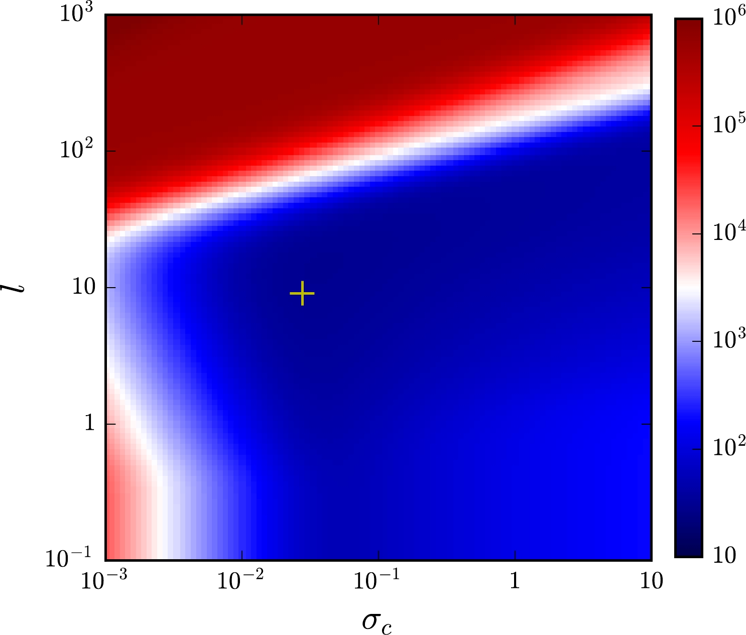
Figure 2. (color online) Heatmap of the NLL probability as a function of the hyperparameters
$ \sigma_{c} $ and l, where the minimum is labeled with a cross.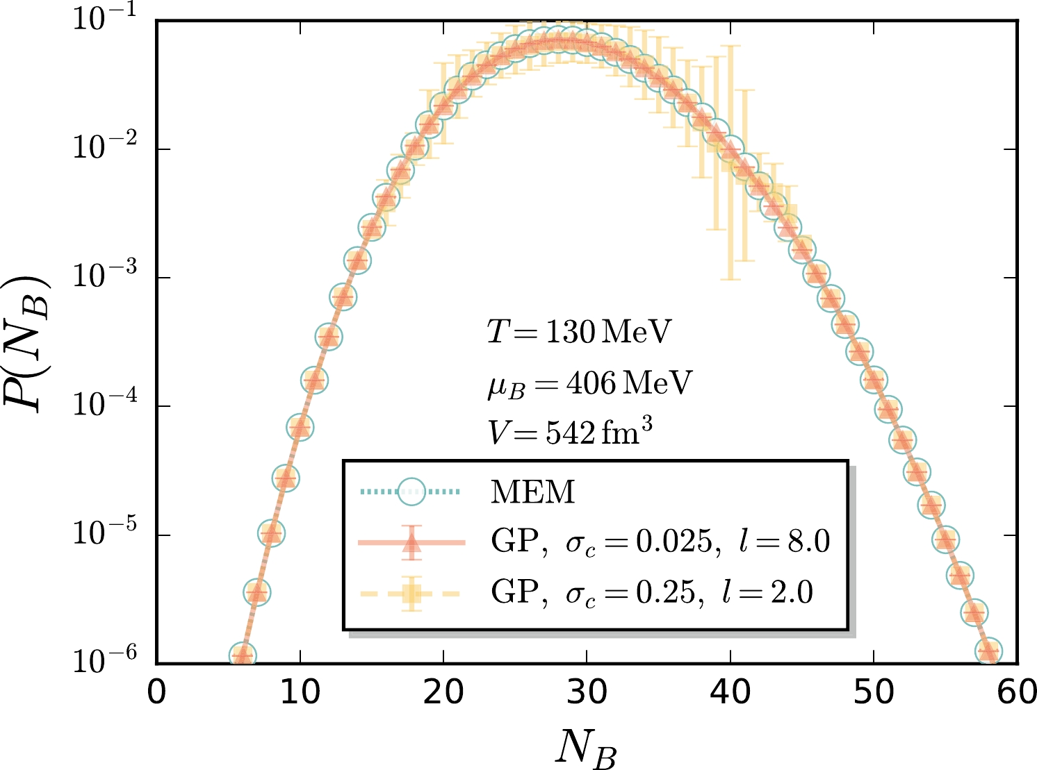
Figure 3. (color online) Baryon number distributions reconstructed from the first four-order cumulants obtained in fRG [31] with
$ T=130 $ MeV,$ \mu_B=406 $ MeV, and$V=542~ {\rm{fm}}^3$ by means of the GP. The NLL function is minimized with the hyperparameters$ \sigma_{c}=0.025 $ and$ l=8.0 $ . The distribution with$ \sigma_{c}=0.25 $ and$ l=2.0 $ and that reconstructed through the MEM are presented for comparison. -
In this section, we use the MEM and GP to reconstruct baryon number distributions across the chiral phase transition, or more exactly, the chiral crossover, with the increase of the temperature at a fixed value of the baryon chemical potential. The employed baryon number susceptibilities of the first four orders are shown in Fig. 4, which are calculated within the fRG approach [31]. Here, we choose the baryon chemical potential
$ \mu_{B}=406 $ MeV, that is around the value of the chemical freeze-out$ \mu_{B} $ with the collision energy$\sqrt{s_{NN}}=7.7$ GeV at RHIC. Then, the relevant pseudo-critical temperature of the chiral crossover is around$ T_{{\rm{pc}}}\sim 137 $ MeV. Four slices of temperature indicated by different symbols as shown in Fig. 4 are chosen. One is smaller than$ T_{{\rm{pc}}} $ a bit$ T=130 $ MeV, and the three others are in the chiral symmetric phase.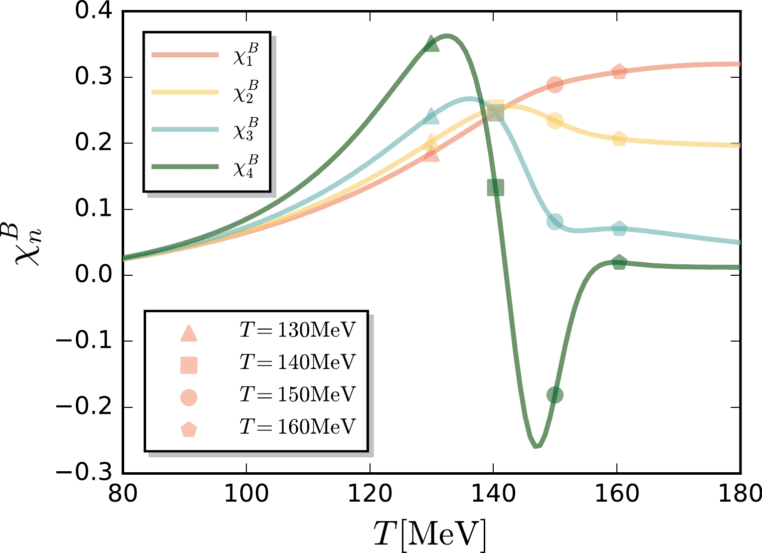
Figure 4. (color online) Baryon number susceptibilities of the first four orders as functions of the temperature T with the baryon chemical potential
$ \mu_{B}=406 $ MeV, obtained in the fRG computations [31]. Susceptibilities at four values of temperature are employed to reconstruct the baryon number distributions in Fig. 5.The baryon number distributions corresponding to the four adopted temperatures in Fig. 4 are shown in Fig. 5. Both the MEM and GP are used to reconstruct the distributions, whose results are denoted by the triangles and circles, respectively. It can also be observed that these two methods give rise to consistent distributions. For the case of
$ T=130 $ MeV, i.e., in the hadronic phase and near the chiral phase transition, it is intriguing to compare the reconstructed baryon number distribution with the hadronic Skellam distribution [53]. The Skellam distribution is completely determined by the first two order cumulants, expressed as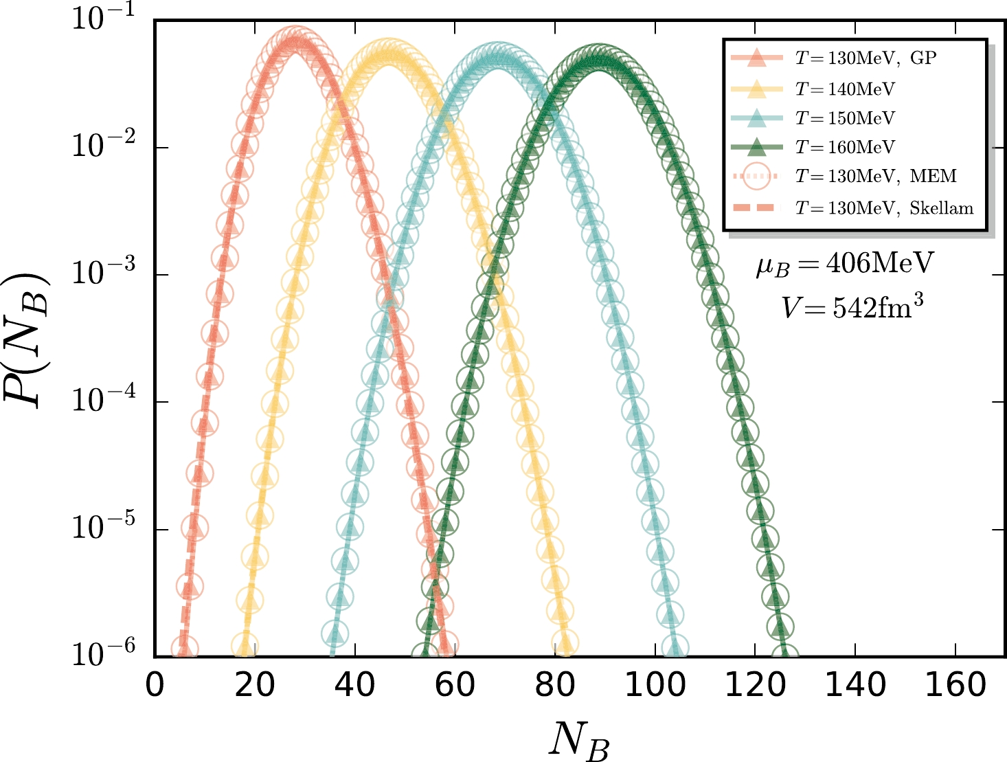
Figure 5. (color online) Baryon number distributions reconstructed from the cumulants in Fig. 4 at four values of temperature with
$ \mu_{B}=406 $ MeV, where the volume is chosen as$V=542~ {\rm{fm}}^{3}$ . Results of both the MEM and GP are presented. The errors for the distributions that can be computed from the GP are not shown because they are too small to be visible. The Skellam distribution at$ T=130 $ MeV is also shown for comparison.$ P(N_B)=\left(\frac{b}{\bar{b}}\right)^{N_B / 2} I_{N_B}\Big(2 \sqrt{b \bar{b}}\Big)\exp\big[-(b+\bar{b})\big]\, , $

(34) with
$ b=\kappa_{2}+\kappa_{1} $ and$ \bar{b}=\kappa_{2}-\kappa_{1} $ being the mean number of baryons and anti-baryons, respectively.$ I_{N_B} $ in Eq. (34) is the modified Bessel function of the first kind. The Skellam distribution of$ T=130 $ MeV is shown in Fig. 5 by the red dashed line. It is deduced that the reconstructed distribution is consistent with the Skellam distribution except that there is a slight deviation in the left tail of the distribution because the temperature is in the proximity of$ T_{{\rm{pc}}} $ .If Eq. (1) is modified as such
$ \langle(\delta N_{B})^{n}\rangle=\sum\limits_{P(N_{B})\geq P_{{\rm{cut}}}}(\delta N_{B})^{n}P(N_{B})\, , $

(35) that is, a cut for the summation of
$ N_{B} $ is implemented, it is possible to determine the dependence of the cumulants on the cut$ P_{{\rm{cut}}} $ , which would reveal important information, such as the importance of the tail of the distribution for different order cumulants. In Fig. 6, the cumulants of the first four orders are shown as functions of the cut$ P_{{\rm{cut}}} $ for the four values of temperature, based on the reconstructed baryon number distributions in Fig. 5. Because the MEM and the GP have almost the same distributions, we do not distinguish them here. It is clearly shown in Fig. 6 that with the increase of the order of cumulants, the saturation$ P_{{\rm{cut}}} $ , i.e., the$ P_{{\rm{cut}}} $ where the curve of$ \kappa_n $ becomes a horizontal line, decreases remarkably. For example,$ \kappa_1 $ saturates at$ P_{{\rm{cut}}}\sim10^{-2} $ ,$ \kappa_2 $ $ \sim10^{-3} $ ,$ \kappa_3 $ $ \sim10^{-4} $ ,$ \kappa_4 $ $ \sim10^{-6} $ . This implies that the statistics in the long tails of the distribution would play a pivotal role in the experimental measurements of high-order cumulants of the net proton number and other conserved charges. Where a higher order is concerned, a longer tail should be considered.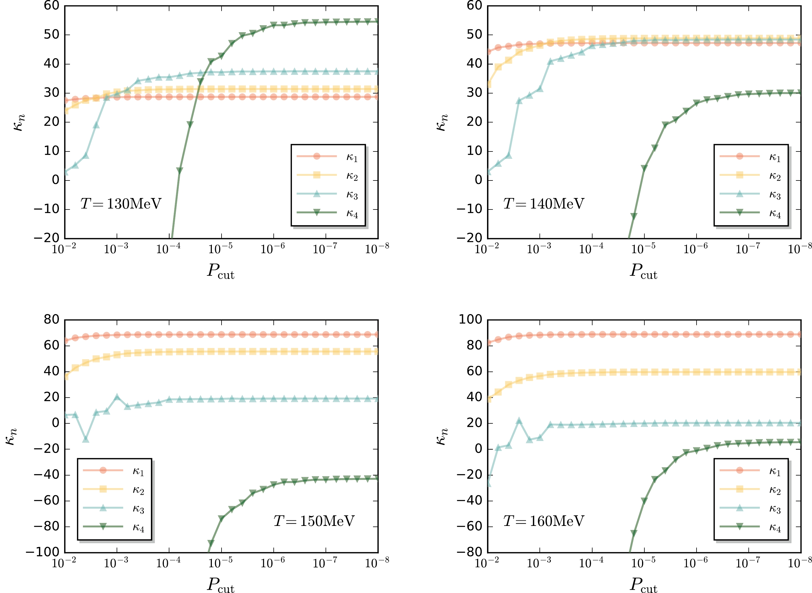
Figure 6. (color online) Cumulants of the first four orders as functions of the cut
$ P_{{\rm{cut}}} $ in Eq. (35) at four temperature values. The reconstructed baryon number distributions in Fig. 5 are used. -
In this section, we apply the two methods, the MEM and GP, to experimental data, for the reconstruction of the distributions. Here, we choose the most important and intriguing fluctuation measurements at the collision energy
$\sqrt{s_{NN}}=7.7$ GeV in the Beam Energy Scan experiment at RHIC, which have been collected in Table 2. Here, the first four order cumulants of the net-proton distributions for central (0−5%) Au+Au collisions are presented [25]. The cumulants measured at$\sqrt{s_{NN}}=7.7$ GeV are believed to play a crucial role in the non-monotonic dependence of the kurtosis on the collision energy observed in experiments. Moreover, it can be observed that the error for the fourth-order cumulant of the experimental data is very large. Therefore, it is very interesting to evaluate the baryon number distributions reconstructed from the measured experimental data, especially the influence of the fourth-order cumulant. It should be noted that we do not distinguish the net-proton number and the net-baron number here, because if the net proton is an ideal proxy for the net baryon in the experimental measurement, the difference between them is a constant factor. In Table 2 we illustrate the theoretical results at$\sqrt{s_{NN}}=$ 7.7 GeV obtained in the fRG [31].$ \kappa_{1} $ 

$ \kappa_{2} $ 

$ \kappa_{3} $ 

$ \kappa_{4} $ 

STAR $ 39.4215{\pm 0.0200} $ 

$ 36.9630{\pm 0.2142} $ 

$ 29.5181{\pm 2.8394} $ 

$ 65.3126{\pm 43.4652} $ 

fRG 39.4662 42.3560 47.6895 57.8462 Table 2. Cumulants of the first four orders of the net-proton distributions for central (0−5%) Au+Au collisions at the collision energy
$\sqrt{s_{NN}}=7.7$ GeV measured by the STAR collaboration [25], as well as the theoretical results for the net-baryon number calculated in fRG [31]. Notably, only the statistical errors of the experimental data are shown here, and we do not include the errors for the fRG results. In the fRG calculations, the chemical freeze-out baryon chemical potential and temperature are$ {\mu_B}_{_{{\rm{CF}}}}=406 $ MeV and$ T_{_{{\rm{CF}}}}=136.2 $ MeV, respectively, at$\sqrt{s_{NN}}=7.7$ GeV. The volume is chosen as$V=542~ {\rm{fm}}^3$ to obtain the same$ \kappa_1 $ for the experiment and theory.In the left panel of Fig. 7 we show the baryon number distributions reconstructed with the MEM and based on the STAR cumulants in Table 2. Because the errors of the first three order cumulants of the STAR data are small, we use their central values. In contrast, the error of the measured
$ \kappa_4 $ is sizable, and it is more reasonable to choose several different values for$ \kappa_4 $ , which are scattered around its central value but within the error. It is deduced that with the increase of$ \kappa_4 $ , there is another peak in the distribution function developed in the region of large$ N_B $ ; the critical value of$ \kappa_4 $ for this behavior, with the values of$ \kappa_1 $ through$ \kappa_3 $ presented in Table 2, is approximately 60, close to the central value measured in the experiments. This unusual behavior of the distribution function is reflected in the dependence of cumulants on the cut defined in Eq. (35) as well. In Fig. 8 the fourth-order cumulant is depicted as a function of the cut. Apparently, it is deduced that when the value of$ \kappa_4 $ is large and above the critical value, the cumulant jumps up to another value after it is already saturated at$ P_{{\rm{cut}}}\sim10^{-6} $ , because the second peak in the distribution function begins to play a role.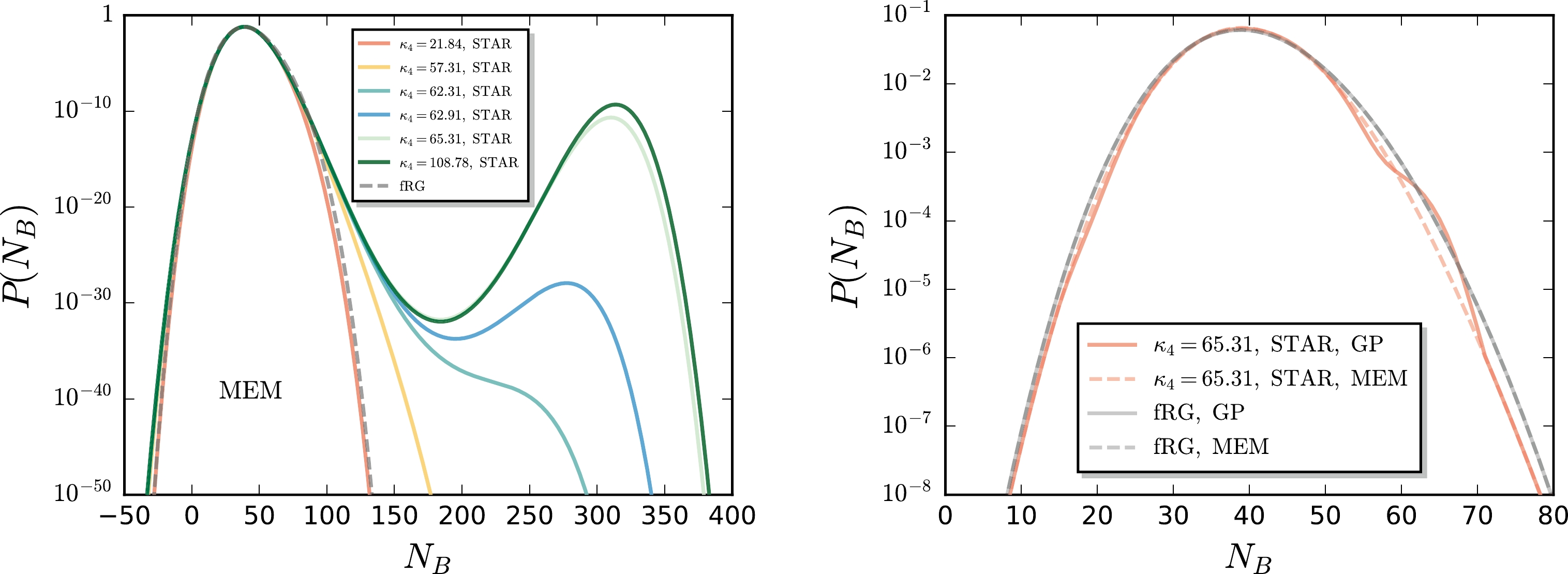
Figure 7. (color online) Left panel: Baryon number distributions reconstructed within the MEM, where the solid and dashed lines denote the results with the STAR and fRG inputs as presented in Table 2, respectively. Here,
$ \kappa_1 $ ,$ \kappa_2 $ ,$ \kappa_3 $ for the STAR data are chosen to be their central values, and$ \kappa_4 $ is varied around its central value but within its error. Right panel: Comparison between the baryon number distribution reconstructed with the GP and that with the MEM for both the STAR and fRG inputs.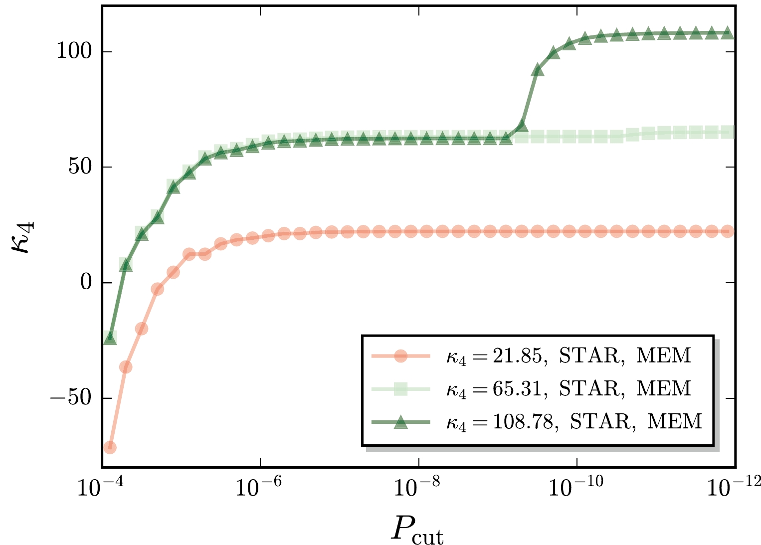
Figure 8. (color online) Fourth-order cumulant as a function of the cut
$ P_{{\rm{cut}}} $ in Eq. (35), where the baryon number distributions of the STAR data with three values of$ \kappa_4 $ , shown in the left panel of Fig. 7, are used. The MEM is employed to reconstruct the distributions.We also use the GP to reconstruct the distribution function based on the STAR data. Unfortunately, reliable calculations in the region of
$ P(N_B)\lesssim 10^{-10} $ are still not accessible at the moment in the GP, where a boundary condition is implemented as discussed above, and thus it is not possible to evaluate the second peak in the GP. However, we show the reconstructed distribution function of the STAR data within the GP in the right panel in Fig. 7. It is observed that it is not consistent with the MEM result, and it can be observed that there is a kink in the curve of GP for the STAR data when$ N_B \in (50, 70) $ . In contrast, for the fRG cumulants in Table 2, both the GP and MEM produce almost identical baryon number distributions as shown in the right panel of Fig. 7, and there is no second peak for the MEM reconstruction as shown in the left panel of Fig. 7.What can we learn from the results of the reconstructed baryon number distributions based on the experimental data above? Certainly, the behavior of a baryon number distribution with two or multiple peaks is odd or anomalous. Given some general assumptions, such as the maximum entropy principle, if a baryon number distribution has an unusual behavior, e.g., multiple peaks, one may refer to this as unnaturalness, which in turn can be used to constrain the cumulants of the net-baryon or net-proton number distributions measured in the experiments. For the inconsistency in
$ P(N_{B}) $ between the GP and MEM methods shown in the right panel of Fig. 7, this indicates an inconsistency among the experimental fluctuations$ \kappa_{1}-\kappa_{4} $ used in reconstructing the distributions. This inconsistency behavior could potentially originate from the experimental data itself, or from limitations due to the insufficient number of data points used for reconstruction. We will investigate this in the future. -
In this work, we employed two methods, the maximum entropy method and the Gaussian process regression, which are both well-suited for the treatment of inverse problems, to reconstruct net-baryon number distributions based on a finite number of cumulants of the distribution.
Owing to the property of convex optimization, we could obtain an analytic function of baryon number distribution within the approach of MEM. In the GP, the hyperparameters in the kernel function were determined by minimizing the negative logarithm likelihood function, which allowed us to extract both the central value and variance of
$ P(N_B) $ for each value of$ N_B $ .We used the MEM and GP to reconstruct baryon number distributions across the chiral phase transition by employing the cumulants calculated in the fRG. It was deduced that the two different approaches, MEM and GP, produce almost identical distribution functions for the fRG inputs. The dependence of cumulants on the cut of the distribution function
$ P_{{\rm{cut}}} $ , i.e., the minimum value of$ P(N_B) $ taken into account in the computation of cumulants, was evaluated. We observed that the saturation$ P_{{\rm{cut}}} $ decreased significantly with the increase of the order of cumulants. This implies that in the experimental measurements of high-order cumulants of the net proton number and other conserved charges, the long tails of the distribution would play a crucial role. Where a higher order is concerned, a longer tail should be considered.Finally, we applied the MEM and GP to the experimentally measured cumulants at the collision energy
$\sqrt{s_{NN}}=$ 7.7 GeV. The values of$ \kappa_1 $ through$ \kappa_3 $ were fixed at their central values, and the value of$ \kappa_4 $ was varied around its central value and within its error. The calculation of MEM showed that with the increase of$ \kappa_4 $ , there is another peak in the distribution function developed in the region of large$ N_B $ . Moreover, the reconstructed distribution function of the STAR data within the GP is not consistent with the MEM result. This unnaturalness observed in the reconstructed distribution function could be used to constrain the cumulants measured in the experiments. -
We thank Xiaofeng Luo for the discussions.
Reconstruction of baryon number distributions
- Received Date: 2023-05-20
- Available Online: 2023-10-15
Abstract: The maximum entropy method (MEM) and Gaussian process (GP) regression, which are both well-suited for the treatment of inverse problems, are used to reconstruct net-baryon number distributions based on a finite number of cumulants of the distribution. Baryon number distributions across the chiral phase transition are reconstructed. It is deduced that with the increase of the order of cumulants, distribution in the long tails, i.e., far away from the central number, would become increasingly important. We also reconstruct the distribution function based on the experimentally measured cumulants at the collision energy


 DownLoad: