-
The standard cosmological model, known as the ΛCDM model, is based on the theory of general relativity and the assumption of the cosmological principle. The cosmological principle extends the Copernican principle and postulates that the universe is statistically homogeneous and isotropic on large scales. This assumption on the large-scale structure of the universe is supported by the approximate isotropy of cosmic microwave background (CMB) radiation observed by, e.g., the Wilkinson Microwave Anisotropy Probe (WMAP) [1, 2] and Planck satellites [3, 4]. However, the cosmological principle also confronts severe challenges from other observations on the large-scale structure. These challenges include the alignment of quasar polarization vectors on large scales [5], spatial variations of fine-structure constant [6, 7], and alignments of low multipoles in the CMB angular power spectrum [8−10]. These abnormal phenomena suggest that our universe may not be isotropic but instead possess anisotropic characteristics. In addition, the largest observed anisotropy in the CMB is the dipole, with an amplitude of approximately
$ 10^{-3} $ , pointing toward the direction$(l,b)= (264^{\circ}, 48^{\circ})$ in the galactic coordinates [8, 11, 12]. All these imply that our universe may deviate from the standard ΛCDM model. Particularly, the Hubble tension problem [13, 14], i.e., the discrepancy between the Hubble constant values measured from the local distance ladders and from the CMB, further poses severe challenges to the standard cosmological model.Since the discovery of a dipole signal in a dataset of 100 type Ia supernovae (SNe Ia), which is consistent with the CMB dipole at a confidence level of more than 2σ [15], various samples of SNe Ia have been used to investigate the potential anisotropy of the universe [16−30]. Using the Union2 dataset, Antoniou & Perivolaropoulos [16] employed the hemisphere comparison method and identified a maximum dark energy dipole direction pointing toward
$ (l,b)=(309^{\circ},18^{\circ}) $ . Utilizing the same dataset but employing the dipole fitting method, Mariano & Perivolaropoulos [7] found a dark energy dipole direction pointing toward$ (l, b) = (309.4^{\circ}, -15.1^{\circ}) $ . Furthermore, Zhao et al. [18] divided the Union2 dataset into 12 subsamples and discovered a dipole in the deceleration parameter at a confidence level exceeding 2σ. A dipole at the level of$ 2\sigma $ was also found in the Union2.1 dataset [21, 22]. However, with the JLA sample, Lin et al. [23] found no significant deviations from the cosmological principle (see also [24−26]). The much larger Pantheon compilation was also utilized to probe the dipole of the universe. Chang et al. [29] found that the dipole anisotropy is very weak in three dipole-modulated cosmological models. In contrast, Horstmann et al. [30] found that the direction of solar motion inferred from Pantheon is consistent with the dipole direction inferred from the CMB. In conclusion, whether our universe is anisotropic or not is still in extensive debate. Therefore, conducting more thorough investigations using high-quality SNe Ia samples before drawing firm conclusions is important.Recently, Scolnic et al. [31] compiled the most up-to-date SNe Ia dataset, including 1701 light curves from 1550 unique SNe Ia observed in 18 different surveys. The dataset covers a wide redshift range of
$ 0.001<z<2.3 $ . Particularly, the SNe Ia at$ z<0.01 $ in the Pantheon+ sample are valuable for analyzing anisotropy in the low-redshift universe. Sorrenti et al. [32] investigated the dipole signal using subsamples of the full Pantheon+ sample based on different low-redshift cutoffs. Their results show that the amplitudes of the dipole signal roughly agree with the CMB dipole, independent of the redshift cutoffs. However, the dipole directions are significantly different from the CMB dipole. In another study, McConville & Colg$ \acute{a} $ in [33] analyzed the anisotropic variation of the Hubble constant using two subsamples of the full Pantheon+ sample in the redshift ranges of$ 0.0233 < z < 0.15 $ and$ 0.01 < z < 0.7 $ , respectively. They found that the Hubble constant is significantly larger in a hemisphere encompassing the CMB dipole direction. However, the variation of the Hubble constant is not sufficiently large to reconcile the Hubble tension problem.These recent investigations highlight the importance of exploring anisotropy using the most updated and comprehensive SNe Ia datasets, such as the Pantheon+ sample, and reveal interesting discrepancies in the dipole directions compared to those of the CMB observations. Further analysis and scrutiny are necessary to fully understand the implications and establish more robust conclusions regarding the presence of anisotropy in the universe. In this study, we will further investigate the possible anisotropy hiding in the Pantheon+ compilation with the dipole fitting method. In contrast to the study by Sorrenti et al. [32], who attributes the anisotropy to the peculiar motion of our solar system with respect to CMB, we directly parameterize the anisotropy in the dipole form. If the anisotropy purely originates from the peculiar motion, the dipole of Pantheon+ is expected to be aligned with the dipole of the CMB, and the dipole signal should be more evident at low redshift. Therefore, we also investigate the anisotropy by dividing the full sample into several subsamples according to redshift. Notably, our method to divide the subsamples is different from that of Sorrenti et al. [32]. We divide the full sample into subsamples using various high-redshift cutoffs, in contrast to the low-redshift cutoffs used by Sorrenti et al. [32]. Comparing the low-redshift SNe with the high-redshift SNe, the former is expected to be more substantially affected by the peculiar motion. Therefore, our research places greater emphasis on the low-redshift subset.
The rest of this paper is arranged as follows. In Sec. II, we introduce the data and methodology used to test the anisotropy of the universe. The results are illustrated in Sec. III. Finally, a discussion and conclusions are given in Sec. IV.
-
SNe Ia serve as ideal standard candles and are widely utilized to constrain the cosmological parameters, especially to investigate the anisotropy of the universe. Recently, Scolnic et al. [31] published the most up-to-date compilation of SNe Ia data, known as the Pantheon+ compilation, which is the updated version of the previous Pantheon compilation [34]. One major difference between Pantheon+ and Pantheon is that the former contains much more low-redshift SNe than the latter, thus allowing us to probe the low-redshift universe more thoroughly. The Pantheon+ compilation consists of 1701 light curves from 1550 unique SNe Ia, covering a redshift range of
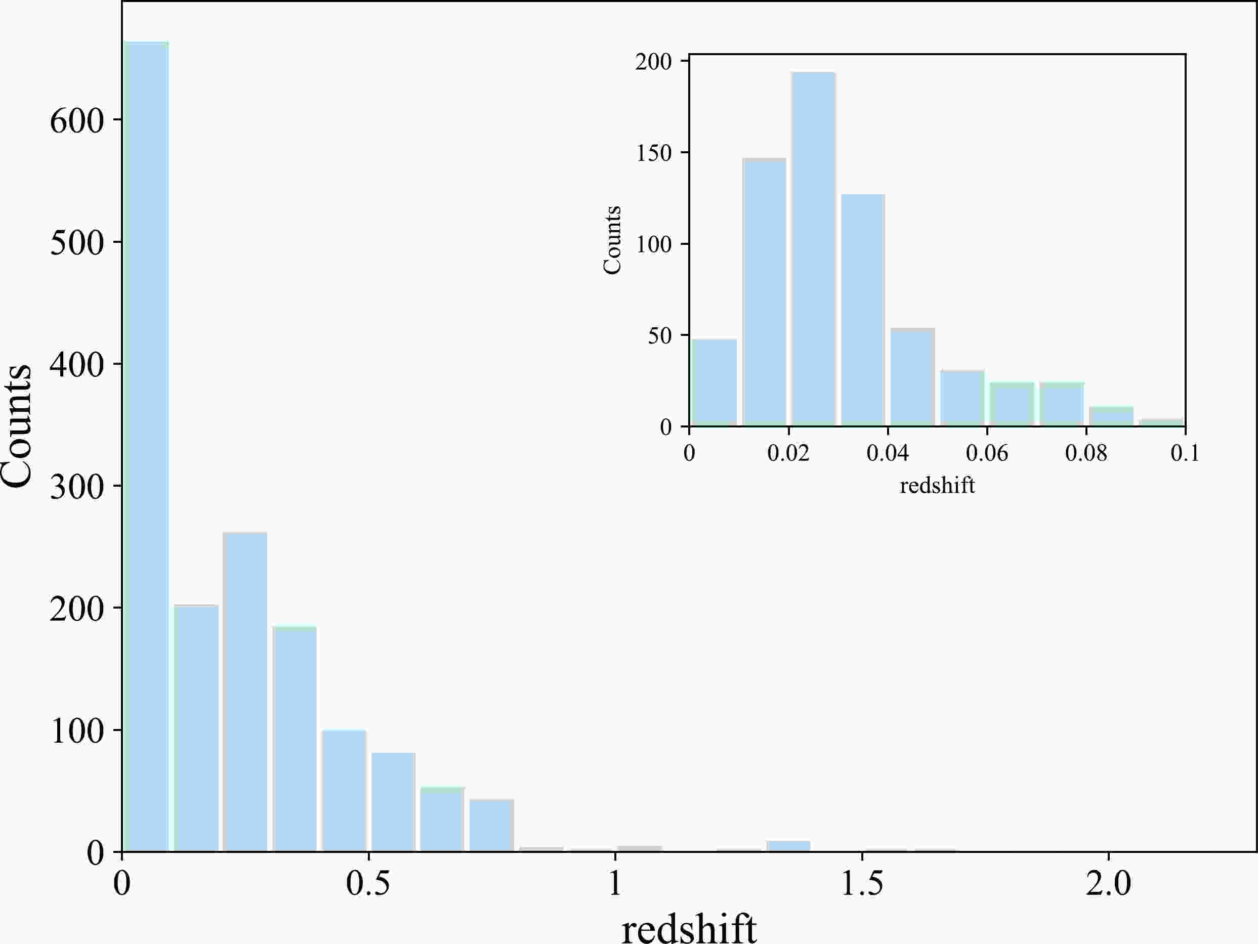
$ 0.001<z<2.3 $ . The redshift distribution of the Pantheon+ dataset is illustrated in Fig. 1. This figure demonstrates that the majority of SNe are concentrated at a low redshift range ($ z<0.1 $ ), while at a high redshift range ($ z>0.8 $ ), the data points are very sparse. To provide a clearer view of this concentration, the inset of Fig. 1 specifically highlights the redshift distribution below 0.1. Additionally, in Fig. 2, we plot the sky positions of the Pantheon+ SNe in the galactic coordinates, which reveals an inhomogeneous distribution, with a large number of data points concentrated near the celestial equator (see the red-solid line in Fig. 2).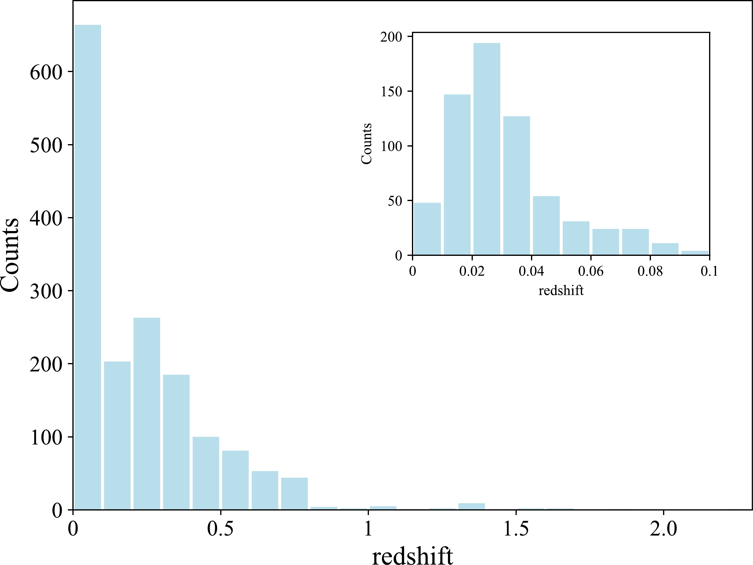
Figure 1. (color online) Redshift distribution of the Pantheon+ SNe. Data points are very sparse at
$ z>0.8 $ . The inset is the redshift distribution of the low-redshift ($ z<0.1 $ ) SNe.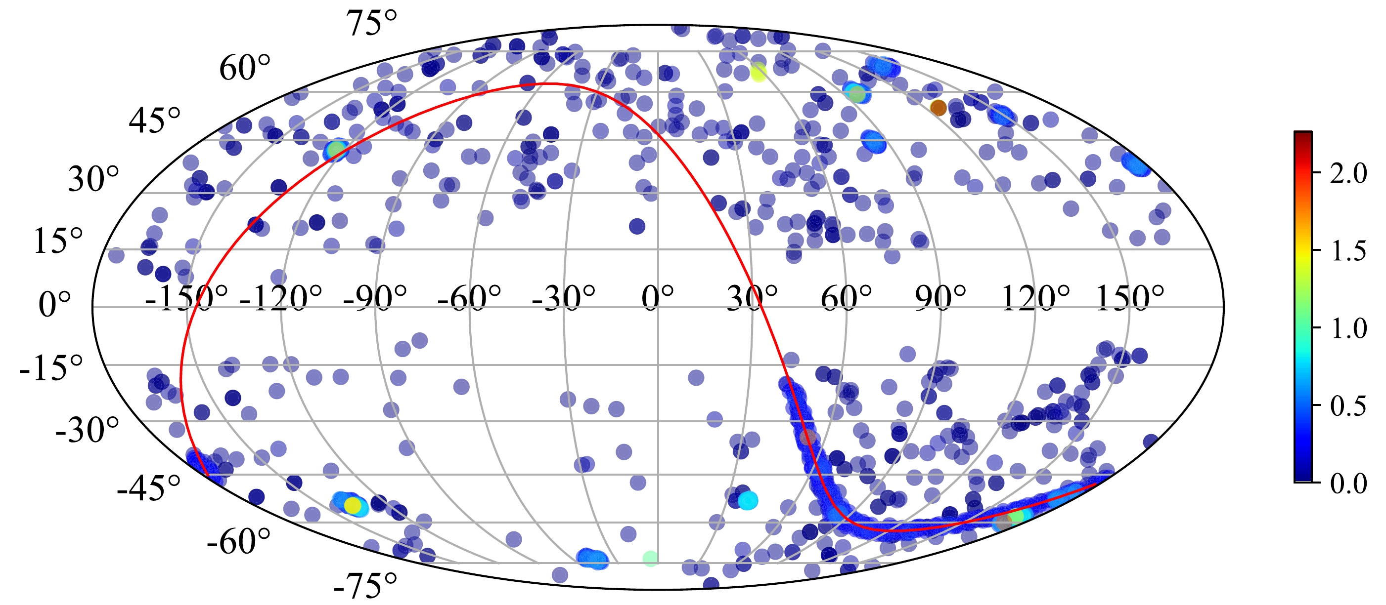
Figure 2. (color online) Sky position of the Pantheon+ SNe in the galactic coordinates colored according to the redshift. The red-solid line is the celestial equator.
The observed distance modulus
$ \mu_{\rm obs} $ is derived from the light curve parameters using a modified version of the Tripp formula [35]:$ \begin{array}{*{20}{l}} \mu_{\rm obs}=m_B-M+\alpha x_1-\beta c_1-\delta_{\rm bias}+\delta_{\rm host}, \end{array} $

(1) where
$ m_B $ represents the apparent magnitude in the B-band, and M corresponds to the absolute magnitude. The parameter$ x_1 $ is associated with the stretch of the light curve width, and$ c_1 $ represents the color parameter influenced by the intrinsic color and dust effects. The nuisance parameters α and β account for the link between the stretch$ x_1 $ and color$ c_1 $ with the luminosity.$ \delta_{\rm bias} $ and$ \delta_{\rm host} $ represent correction terms, where$ \delta_{\rm bias} $ accounts for the selection biases from simulations,$ \delta_{\rm host} $ considers the contribution of the host galaxy mass of the SNe Ia. After calibration using the BEAMS with bias corrections (BBC) method [36], the Pantheon+ dataset provides the corrected magnitude$ m_{\rm obs} $ , along with the corresponding covariance matrix. The observed distance modulus is then expressed as$ \mu_{\rm obs}=m_{\rm obs}-M $ . The details of the Pantheon+ dataset can be found in Scolnic et al. [31].In a spatially flat universe, the dimensionless distance modulus at a given redshift z can be expressed as
$ \mu(z)=5\log_{10}\frac{d_L(z)}{\rm Mpc}+25, $

(2) where
$ d_L $ represents the luminosity distance and is measured in units of Mpc. In the framework of the standard ΛCDM model, the luminosity distance takes the following form:$ d_L(z)=(1+z)\frac{c}{H_0}\int^z_0\frac{{\rm d}z}{\sqrt{\Omega_{\rm M}(1+z)^3+\Omega_{\Lambda}}}, $

(3) where c denotes the speed of light,
${H_0}$ represents the Hubble constant, typically parameterized in terms of a dimensionless parameter$h\equiv H_0/ (100\; {\rm km/ {\rm s/Mpc}})$ ; and$ \Omega_{\rm M} $ and$ \Omega_{\Lambda}=1-\Omega_{\rm M} $ denote the dimensionless densities of matter and dark energy, respectively.The dipole fitting method, first introduced by Mariano et al. [7], is utilized to investigate the anisotropy of the universe. This method fits the observational data using a dipole model directly. According to the dipole fitting method, a dipole modulation is introduced to the theoretical distance modulus in the isotropic ΛCDM model, given by the following form:
$ \begin{array}{*{20}{l}} \mu_D(z)=\mu_{\rm iso}(z)\left[1+D({\hat{\boldsymbol{n}}} \cdot {\hat{\boldsymbol{p}}})\right]. \end{array} $

(4) Here,
$ \mu_{\rm iso}(z) $ represents the distance modulus in the isotropic ΛCDM model determined by Eq. (2), D is the amplitude of the dipole,$ {\hat{\boldsymbol{n}}} $ is the direction of the dipole, and$ {\hat{\boldsymbol{p}}} $ is the unit vector pointing toward the SNe Ia. In galactic coordinates, the two unit vectors$ {\hat{\boldsymbol{n}}} $ and$ {\hat{\boldsymbol{p}}} $ can be parameterized using the galactic longitude l and latitude b in the following manner:$ {\hat{\boldsymbol{n}}}=\cos(b_0)\cos(l_0){\hat{\boldsymbol{i}}}+\cos(b_0)\sin(l_0){\hat{\boldsymbol{j}}}+\sin(b_0){\hat{\boldsymbol{k}}}, $

(5) $ {\hat{\boldsymbol{p_i}}}=\cos(b_i)\cos(l_i){\hat{\boldsymbol{i}}}+\cos(b_i)\sin(l_i){\hat{\boldsymbol{j}}}+\sin(b_i){\hat{\boldsymbol{k}}}, $

(6) where
$ {\hat{\boldsymbol{i}}} $ ,$ {\hat{\boldsymbol{j}}} $ , and$ {\hat{\boldsymbol{k}}} $ represent the unit vectors along the three axes of the Cartesian coordinates, and ($ l_0 $ ,$ b_0 $ ) and ($ l_i $ ,$ b_i $ ) represent the direction of the dipole and direction of the i-th SN in the galactic coordinates, respectively. In the Pantheon+ dataset, the SNe positions are provided in the equatorial coordinates. In order to directly compare with other works, we transform the equatorial coordinates$ ({\rm RA, DEC}) $ to the galactic coordinates ($ l,b $ ) using the formulae given in Ref. [37].The free parameters in our analysis consist of the matter density
$ \Omega_{\rm m} $ , absolute magnitude M, dimensionless Hubble constant h, dipole amplitude D, and dipole direction$ (l_0,b_0) $ . Therein, the absolute magnitude M and dimensionless Hubble constant h cannot be simultaneously constrained using SNIa data alone due to their degeneracy. Fortunately, the absolute magnitude M can also be refined by establishing an absolute distance scale, employing primary distance anchors such as Cepheids. The Pantheon+ dataset has extended the lower redshift boundary of SNe Ia to 0.001, which encompasses primary distance indicators found in Cepheid host galaxies. The degeneracy between M and h is eliminated by combining the measurements from the SH0ES Cepheid and SNe data. As a result, M and h can be constrained simultaneously. Following the methodology outlined by Brout et al. [38], the best-fitting parameters are determined by maximizing the likelihood function, which is related to the$ \chi^2 $ by$ \begin{array}{*{20}{l}} -2\ln(\mathcal{L})=\chi^2=\Delta{\boldsymbol{\mu}}^{T}{\boldsymbol{C}}^{-1}\Delta{\boldsymbol{\mu}}, \end{array} $

(7) in which
$ {\boldsymbol{C}} $ represents the total covariance matrix, which combines the statistical and systematic covariance matrices.$ \Delta{\boldsymbol{\mu}} $ denotes the residual vector of the distance modulus, where the i-th element is defined as$ \Delta\mu_i= \left\{ \begin{array}{*{20}{l}} \mu_{{\rm{obs}},i}-\mu_{{\rm{ceph}},i},& i\in {\rm{Cepheid}} \ {\rm{hosts}},\\ \mu_{{\rm{obs}},i}-\mu_{D,i},& {\rm{otherwise}}. \end{array} \right. $

(8) Here,
$ \mu_{{{\rm{ceph}}},i} $ corresponds to the calibrated distance to the host galaxy determined from the Cepheid measurements, while$ \mu_{{{\rm{obs}}},i} $ and$ \mu_{D,i} $ are determined by Eq. (1) and Eq. (4), respectively. -
We employ the Markov Chain Monte Carlo (MCMC) method, specifically the affine-invariant MCMC ensemble sampler provided by the publicly available Python package
$\textsf{emcee}$ 1 [39], to perform the parameter fitting. The posterior probability density functions (PDFs) of the free parameters are calculated using this approach. For each parameter, we assume a flat prior distribution as follows:$ \Omega_{\rm M}\sim[0, 1] $ ,$ M\sim[-21.0,-18.0] $ ,$ h\sim[0.6,0.8] $ ,$ D\sim[0,0.01] $ ,$ l_0\sim[-180^{\circ},180^{\circ}] $ 2 , and$ b_0\sim[-90^{\circ},90^{\circ}] $ .First, we use the full Pantheon+ sample to constrain the free parameters of the dipole-modulated ΛCDM model. The full sample contains 1701 data points in the redshift range
$ z<2.3 $ , including 77 SNe in galaxies hosting Cepheids. The constraints on the parameters are summarized in the first row of Table 1. The left panel of Fig. 3 shows the corresponding two-dimensional confidence contours and one-dimensional posterior PDFs for the parameters. In the dipole-modulated ΛCDM model, the background parameters$ \Omega_{\rm M} $ , M, and h are tightly constrained as$ \Omega_{\rm M}=0.334^{+0.018}_{-0.018} $ ,$ M=-19.248_{-0.030}^{+0.029} $ , and$ h=0.735_{-0.010}^{+0.010} $ , which are consistent with those obtained from the isotropic flat ΛCDM model [38] within 1σ uncertainty. Regarding the dipole component, the anisotropic signal is weak in the full Pantheon+ sample. The 68% upper limit of the dipole amplitude is constrained to be$ D<0.3\times 10^{-3} $ , and the dipole direction points toward$ (l_0,b_0)=(326.3_{\ -49.5^{\circ}}^{\circ+82.4^{\circ}},-10.4_{\ -40.0^{\circ}}^{\circ+37.9^{\circ}}) $ . The small upper limit of the dipole amplitude and the large uncertainty on the dipole direction indicate that the full Pantheon+ dataset is well consistent with a large-scale isotropic universe.Sample N $ \Omega_m $ 

M h $ D/10^{-3} $ 

$ l_0[^{\circ}] $ 

$b_0/(^{\circ})$ 

$ z<2.3 $ 

1701 $ 0.334_{-0.018}^{+0.018} $ 

$ -19.248_{-0.030}^{+0.029} $ 

$ 0.735_{-0.010}^{+0.010} $ 

$<0.3 $ 

$ 326.3_{-49.5}^{+82.4} $ 

$ -10.4_{-40.0}^{+ 37.9} $ 

$ z<0.7 $ 

1626 $ 0.348_{-0.021}^{+0.022} $ 

$ -19.245_{-0.030}^{+0.030} $ 

$ 0.735_{-0.010}^{+0.010} $ 

$<0.4 $ 

$ 320.8_{-42.2}^{+64.5} $ 

$ -12.6_{-35.8}^{+ 29.8} $ 

$ z<0.5 $ 

1492 $ 0.332_{-0.024}^{+0.025} $ 

$ -19.244_{-0.030}^{+0.029} $ 

$ 0.736_{-0.010}^{+0.010} $ 

$<0.5 $ 

$ 320.7_{-40.1}^{+67.3} $ 

$ -13.1_{-33.5}^{+ 29.4} $ 

$ z<0.4 $ 

1392 $ 0.341_{-0.029}^{+0.030} $ 

$ -19.245_{-0.029}^{+0.030} $ 

$ 0.735_{-0.010}^{+0.010} $ 

$<0.4 $ 

$ 317.2_{-50.5}^{+80.2} $ 

$ -3.3_{-35.7}^{+ 43.5} $ 

$ z<0.3 $ 

1207 $ 0.404_{-0.043}^{+0.045} $ 

$ -19.246_{-0.030}^{+0.029} $ 

$ 0.733_{-0.010}^{+0.010} $ 

$<0.7 $ 

$ 315.6_{-31.0}^{+46.3} $ 

$ 12.6_{-22.3}^{+ 39.3} $ 

$ z<0.2 $ 

944 $ 0.446_{-0.073}^{+0.075} $ 

$ -19.246_{-0.030}^{+0.030} $ 

$ 0.732_{-0.010}^{+0.010} $ 

$ 0.7_{-0.4}^{+0.4} $ 

$ 323.7_{-24.9}^{+35.0} $ 

$ 13.2_{-19.2}^{+33.9} $ 

$ z<0.1 $ 

741 $ 0.411_{-0.213}^{+0.235} $ 

$ -19.249_{-0.030}^{+0.030} $ 

$ 0.731_{-0.011}^{+0.011} $ 

$ 1.0_{-0.4}^{+0.4} $ 

$ 334.5_{-21.6}^{+25.7} $ 

$ 16.0_{-16.8}^{+27.1} $ 

$ z<0.07 $ 

702 $ 0.551_{-0.280}^{+0.263} $ 

$ -19.250_{-0.030}^{+0.030} $ 

$ 0.729_{-0.011}^{+0.011} $ 

$ 0.8_{-0.4}^{+0.4} $ 

$ 330.9_{-29.1}^{+34.0} $ 

$ 26.0_{-22.5}^{+34.1} $ 

$ z<0.04 $ 

593 $ 0.344_{-0.245}^{+0.349} $ 

$ -19.250_{-0.030}^{+0.029} $ 

$ 0.730_{-0.011}^{+0.011} $ 

$ 1.0_{-0.4}^{+0.4} $ 

$ 316.4_{-31.3}^{+34.9} $ 

$ 36.4_{-24.1}^{+31.9} $ 

$ z<0.03 $ 

466 $ 0.635_{-0.366}^{+0.261} $ 

$ -19.250_{-0.030}^{+0.029} $ 

$ 0.733_{-0.011}^{+0.011} $ 

$ 1.5_{-0.6}^{+0.6} $ 

$ 322.7_{-21.3}^{+23.5} $ 

$ 16.9_{-17.4}^{+26.4} $ 

$ z<0.02 $ 

272 $ 0.482_{-0.332}^{+0.346} $ 

$ -19.252_{-0.030}^{+0.029} $ 

$ 0.723_{-0.012}^{+0.012} $ 

$ 1.4_{-0.9}^{+0.9} $ 

$ 282.7_{-39.2}^{+56.6} $ 

$ 20.9_{-30.3}^{+38.6} $ 

Table 1. Best-fitting parameters of the dipole-modulated ΛCDM model. The uncertainties are given at the
$ 1\sigma $ confidence level. For the dipole amplitude, the$ 68% $ upper limit is reported when the posterior DPF has no evident peak. The second column lists the number of data points. The galactic longitude$ l_0 $ is converted into the range of$ [0^{\circ},360^{\circ}] $ .
Figure 3. (color online) Posterior PDFs of parameters and two-dimensional confidence contours constrained from the full Pantheon+ sample (left panel) and the
$ z<0.1 $ subsample (right panel). The black dashed lines represent the median value and$ 1\sigma $ uncertainty, and the red dashed line is the$ 1\sigma $ upper limit.In addition to investigating the dipole using the full Pantheon+ dataset, we explore the possible redshift-dependence of the dipole by dividing the dataset into several subsamples. These subsamples are obtained by excluding supernovae with redshift higher than a certain cutoff value
$ z_{\rm c} $ . In other words, a subsample consists of the supernovae with redshift$ z<z_c $ . The cutoff redshift$ z_c $ is chosen from 0.1 to the maximum redshift with an equal step size$ \Delta z=0.1 $ . Since the number of data points in some redshift bins are very sparse, as is seen from Fig. 1, we only consider the subsamples with number differences larger than 100. We finally found six subsamples, with$ z_c=0.1 $ , 0.2, 0.3, 0.4, 0.5, 0.7. The number of data points in each subsample is listed in the second column of Table 1. Notably, all supernovae in galaxies hosting Cepheids are included in each subsample, even if their redshift exceeds the cutoff value. This is because these supernovae are used to determine the absolute magnitude, M, and eliminate the degeneracy between M and h.We constrain the parameters of the dipole-modulated ΛCDM model with each subsample using the same method mentioned above, and the results are summarized in Table 1. Similar to that inferred from the full Pantheon+ sample, it is found that there is no strong evidence for the presence of dipole anisotropy in the subsamples with a cutoff redshift
$ z_{\rm c} $ higher than 0.2. However, the dipole signal emerges in the subsamples with$ z_{\rm c}\leq0.2 $ . In the subsample with$ z<0.2 $ , the dipole amplitude is constrained as$ D=0.7^{+0.4}_{-0.4}\times 10^{-3} $ , pointing toward$ (l_0,b_0)= (323.7_{\ -24.9^{\circ}}^{\circ+35.0^{\circ}},13.2_{\ -19.2^{\circ}}^{\circ+33.9^{\circ}}) $ , which deviates from an isotropic universe at$ >1\sigma $ confidence level. In contrast, in the subsample with$ z<0.1 $ , the dipole signal emerges at the$ >2\sigma $ confidence level, with a dipole amplitude$ D=1.0_{-0.4}^{+0.4}\times 10^{-3} $ , pointing toward$(l_0,b_0)= $ $(334.5_{\ -21.6^{\circ}}^{\circ+25.7^{\circ}}, 16.0_{\ -16.8^{\circ}}^{\circ+27.1^{\circ}})$ . The right panel of Fig. 3 shows the corresponding two-dimensional confidence contours and one-dimensional posterior PDFs for the parameters with this subsample. To facilitate comparison, we also plot the posterior PDFs of the parameters constrained from different subsamples in Fig. 4. As can be seen, the significance of the dipole signal progressively increases with the decrease in$ z_c $ , while the dipole direction is relatively stable.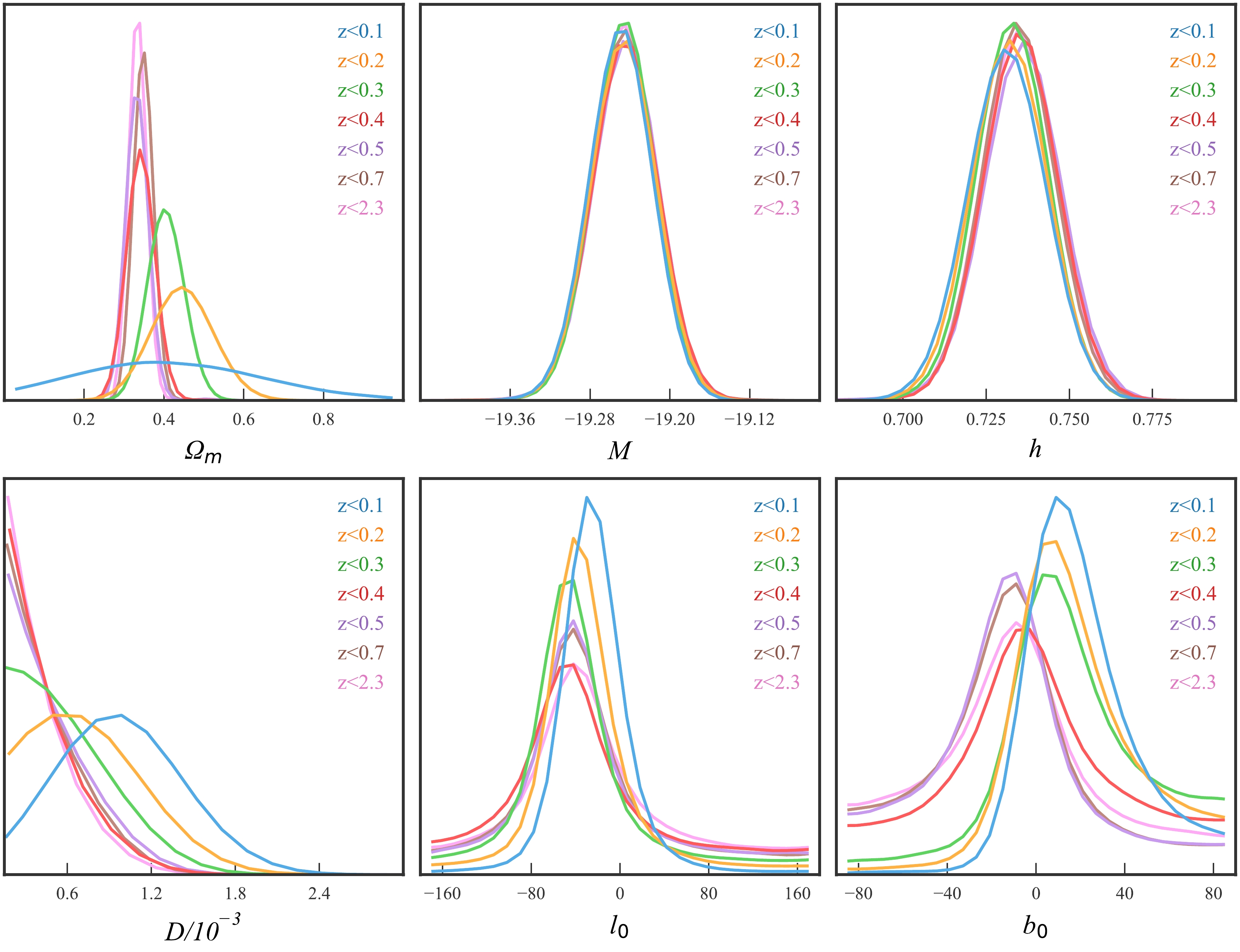
Figure 4. (color online) Posterior PDFs of parameters constrained from different subsamples with
$ z_c\geq 0.1 $ .We note that more than one-third of data points have a redshift below
$ 0.1 $ ( see Fig. 1). In light of the clear dipole signal in the low-redshift range, we perform a thorough examination of the dipole-modulated ΛCDM model with the low-redshift data points by dividing it into several redshift bins. To achieve this, we further divide the$ z<0.1 $ data points into several subsamples using a similar method as before but with a smaller redshift interval of 0.01. We also only consider the subsamples with number differences larger than 100. We finally find four subsamples:$ z<0.02 $ ,$ z<0.03 $ ,$ z<0.04 $ , and$ z<0.07 $ . The constraining results from these subsamples are summarized in the last four columns of Table 1. Because the luminosity distance (see Eq. (3)) is insensitive to the matter density parameter$ \Omega_{\rm M} $ at the low-redshift region, this parameter could not be tightly constrained. The constraints on the other parameters remain consistent across all the subsamples. Especially, the parameters M and h are almost independent of the subsamples. This indicates that the dipole-modulated ΛCDM model provides stable parameter estimation in the low-redshift range. The posterior PDFs of the parameters, constrained from different low-redshift subsamples, are displayed in Fig. 5. These plots further support the existence of an anisotropic signal at the low-redshift region. Notably, the dipole parameters are stable, remaining nearly independent of the specific value of the cutoff redshift$ z_{\rm c} $ , although the uncertainty is large for the lowest-redshift subsample ($ z<0.02 $ ).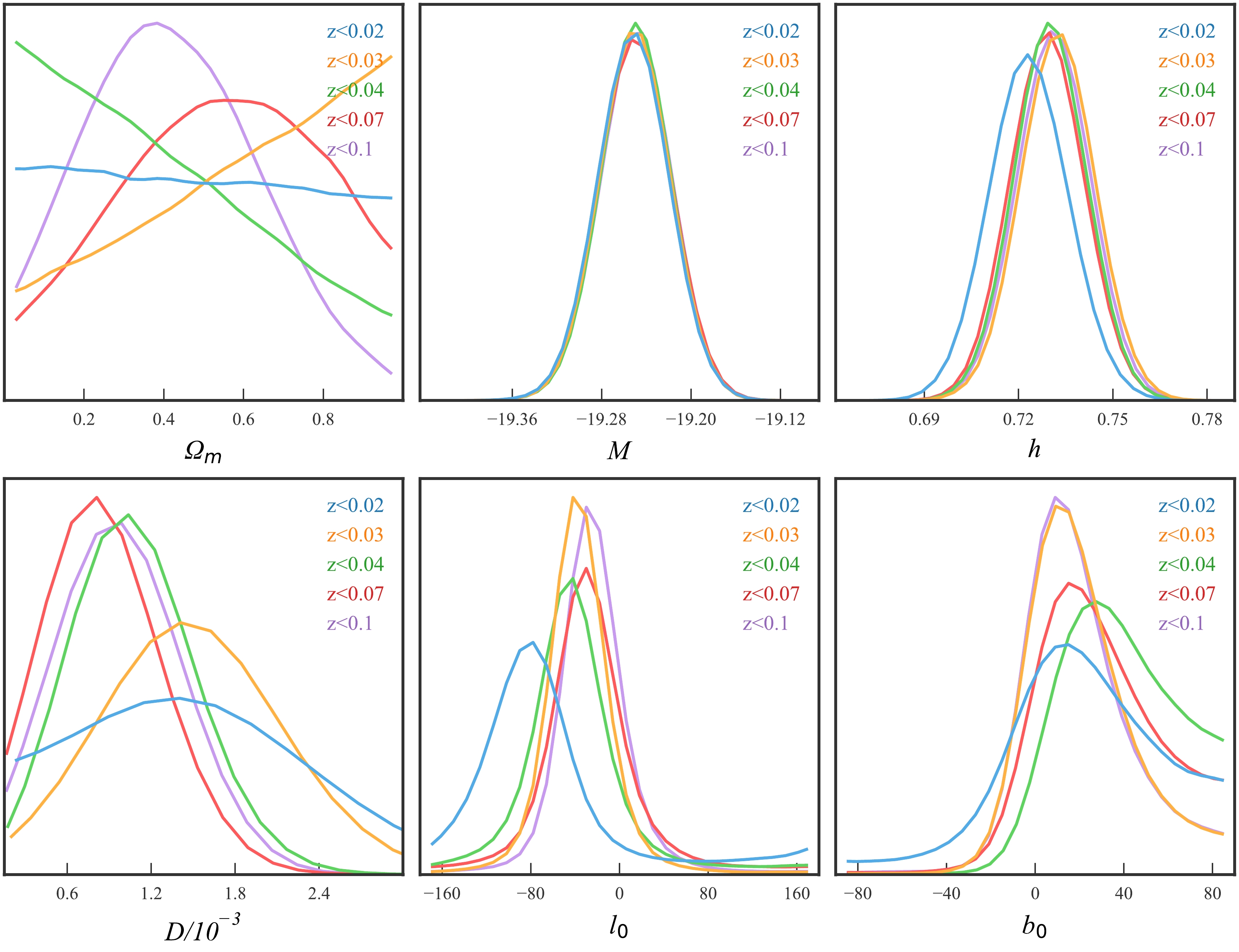
Figure 5. (color online) Posterior PDFs of parameters constrained from different subsamples with
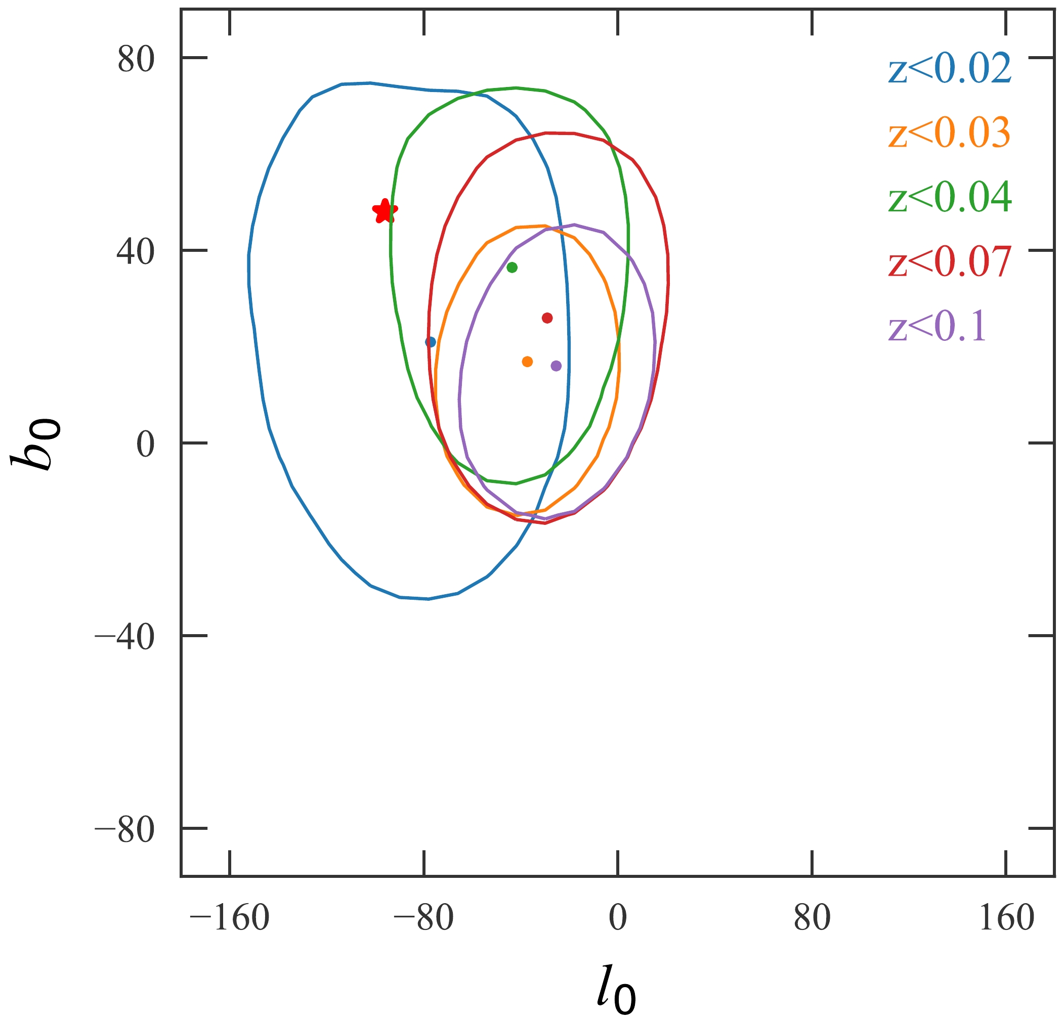
$ z_c\leq 0.1 $ .Figure 6 shows the dipole directions constrained from the low-redshift subsamples. In this figure, the contours represent the 1σ uncertainty regions of the dipole directions. For comparison, the CMB dipole direction pointing toward
$ (l,b)=(264^{\circ},48^{\circ}) $ [12] is also shown using a red star. From this figure, we can clearly see that the dipole directions obtained from different subsamples are consistent. Notably, the dipole directions of all low-redshift subsamples, except for the lowest-redshift subsample ($ z<0.02 $ ), deviate from the CMB dipole at more than the$ 1\sigma $ confidence level. The consistency between the dipole directions of the$ z<0.02 $ subsample and the CMB is mainly due to the large uncertainty of the former. This implies that the anisotropic signal underlying the low-redshift Pantheon data could not be purely explained by the peculiar motion of the local universe. -
In this study, we investigated the possible anisotropy of the universe using the most up-to-date SNe Ia dataset, i.e., the Pantheon+ compilation. We phenomenally constructed a dipole-corrected Hubble diagram based on the spatially flat ΛCDM model and fitted it to the Pantheon+ compilation. We found that the full Pantheon+ compilation is well consistent with an isotropic universe, at the
$ 1\sigma $ upper limit of dipole amplitude$ D<0.3\times 10^{-3} $ . To check the possible redshift dependence of the result, we fitted our model with the low-redshift subsamples ($ z<z_c $ ) of Pantheon+, where$ z_c $ is the cutoff value. It was shown that the anisotropic signal exists only if$ z_c\leq 0.2 $ . Especially for$ z_c=0.1 $ , the anisotropic signal is at the significance level of$ 2\sigma $ , with the dipole amplitude$ D= 1.0_{-0.4}^{+0.4}\times 10^{-3} $ and the dipole direction$ (l,b)=(334.5_{\ -21.6^{\circ}}^{\circ+25.7^{\circ}}, 16.0_{\ -16.8^{\circ}}^{\circ+27.1^{\circ}}) $ . This direction is$ 65^\circ $ away from the CMB dipole,$ (l,b)=(264^{\circ},48^{\circ}) $ [8]. If one naively assumes that the anisotropy is induced by the peculiar velocity, one may expect that the dipole of SNe is aligned with the dipole of CMB. Therefore, the dipole of Pantheon+ seen at$ z<0.1 $ could not be purely explained by the peculiar motion of the local universe.The anisotropy of the universe has been extensively investigated using different groups of SNe Ia. For instance, Mariano & Perivolaropoulos [7] found a dipole in the Union2 dataset, with an amplitude
$ A = (1.3 \pm0.6) \times 10^{-3} $ , pointing toward$ (l, b) = (309.4^{\circ} \pm 18.0^{\circ}, -15.1^{\circ} \pm 11.5^{\circ}) $ . Wang & Wang [21] found a dipole with an amplitude$ A = (1.37 \pm 0.57) \times 10^{-3} $ , pointing toward$ (l, b) = (309.2^{\circ} \pm 15.8^{\circ}, -8.6^{\circ} \pm 10.5^{\circ}) $ in Union2.1. Using the JLA dataset, Lin et al. [23] found that the dipole is well consistent with null, with the amplitude$ A < 1.98 \times 10^{-3} $ , pointing toward$ (l, b) = (316_{\ -110^{\circ}}^{\circ+107^{\circ}}, -5_{\ -60^{\circ}}^{\circ+41^{\circ}}) $ . Zhao et al. [40] found that there is no evidence for the dipole anisotropy in Pantheon, with an amplitude$ A < 1.16 \times 10^{-3} $ , pointing toward$ (l, b) = (306_{\ -125^{\circ}}^{\circ+83^{\circ}}, -34_{\ -55^{\circ}}^{\circ+17^{\circ}}) $ . In this study, we also found that Pantheon+, an updated version of Pantheon, is well consistent with an isotropic universe, with a dipole amplitude$ A < 0.3\times 10^{-3} $ , pointing toward$ (l,b) = (326.3_{\ -49.5^{\circ}}^{\circ+82.4^{\circ}}, -10.4_{\ -40.0^{\circ}}^{\circ+37.9^{\circ}}) $ . The dipoles of Union2 and Union2.1 are at the level of$ \sim 2\sigma $ , while the dipoles of JLA, Pantheon, and Pantheon+ are well consistent with null. We note that the redshift range of the former two datasets is$ 0<z<1.4 $ , while the redshift range of the latter three datasets is$ 0<z<2.3 $ . However, the number of SNe with$ z>1.4 $ is very small. Therefore, the different results are not expected to be caused by the extension of redshift. One reason for the difference may be that the correlation between SNe in Union2 and Union2.1 has been ignored, while the covariance matrix of JLA, Pantheon, and Pantheon+ has been fully considered. Another reason may be that the number of data points almost tripled from Union2 ($ N=557 $ ) to Pantheon+ ($ N=1701 $ ). With the enlargement of the data sample, the anisotropic signal gradually vanishes.The dipole anisotropy of the Pantheon+ has also been studied by Sorrenti et al. [32]. In their paper, the authors attribute the anisotropy to the peculiar motion of our solar system with respect to the CMB frame. The peculiar motion of our solar system induces a redshift correction for each SN, which depends on the position of the SN in the sky. They found the peculiar velocity
$v_0= $ $ 328_{-42}^{+35}\; {\rm km/s} $ , pointing toward$ ({\rm RA,DEC})=(139.4_{\ -8.0^{\circ}}^{\circ+7.2^{\circ}}, 42.0_{\ -6.6^{\circ}}^{\circ+7.2^{\circ}}) $ in equatorial coordinates, which corresponds to the dipole amplitude$ D=v_0/c=(1.1\pm 0.1)\times 10^{-3} $ and dipole direction$ (l,b)=(180^{\circ},45^{\circ}) $ . The well-known CMB dipole has$ v_0=369\pm 0.9\; {\rm km/s} $ , pointing toward$(l,b)= (264^{\circ}, 48^{\circ})$ [12]. Although the amplitudes of peculiar velocity derived from Pantheon+ are well consistent with those of the CMB dipole, the direction is significantly different. They also investigated the dipole anisotropy using subsamples of Pantheon+, with different low-redshift cutoffs$ z_{\rm cut} $ (note that this is different from our study, where we use a high-redshift cutoff, rather than a low-redshift cutoff). They found that the dipole anisotropy is significant only at$ z_{\rm cut}\leq 0.05 $ . This is consistent with our conclusion that the anisotropy only exists at the low redshift region.
Consistency of Pantheon+ supernovae with a large-scale isotropic universe
- Received Date: 2023-07-25
- Available Online: 2023-12-15
Abstract: We investigate the possible anisotropy of the universe using data on the most up-to-date type Ia supernovae, i.e., the Pantheon+ compilation. We fit the full Pantheon+ data with the dipole-modulated ΛCDM model and find that the data are well consistent with a null dipole. We further divide the full sample into several subsamples with different high-redshift cutoffs


 Abstract
 HTML
HTML Reference
 Related
 PDF
PDF






 DownLoad: