


 Abstract
 HTML
HTML Reference
 Related
 PDF
PDF


-
The suppression of
$ J/\psi $ production in relativistic heavy ion collisions is an important signature to identify the quark-gluon plasma [1]. Because of the color screening, the dissociation of$ J/\psi $ in the quark-gluon plasma would lead to a reduction of its production. The bottomonia are also sensitive to the color screening; therefore, the$\Upsilon $ suppression in heavy ion collisions can also be considered as a signature to identify the quark-gluon plasma [2, 3]. Some attempts to analyze the heavy quarkonium absorptions using the effective Lagrangians in meson exchange models have been successful [4−8]. Further, the absorption cross sections can be calculated based on the interactions among the mesons and quarkonia, where the strong coupling constants are taken as an important input parameter. Meanwhile, accurate determination of the strong coupling constants plays an important role in understanding the effects of heavy quarkonium absorptions in hadronic matter [9]. Besides, the coupling constants among heavy quarkonia and heavy mesons are valuable for us to understand the final-state interactions in heavy quarkonium decays [9, 10].The QCD sum rules and the light-cone QCD sum rules are powerful nonperturbative approaches in analyzing the strong coupling constants among the hadrons. In recent years, the strong vertices
$ DD^{*}\pi $ ,$ D^{*}D_{s}K $ ,$ DD_{s}^{*}K $ ,$ BB^{*}\pi $ ,$ B^{*}B_{s}K $ ,$ BB_{s}^{*}K $ ,$ DD\rho $ ,$ DD_{s}K^{*} $ ,$ BB_{s}K^{*} $ ,$ DD^{*}\rho $ ,$ DD^{*}_{s}K^{*} $ ,$ BB^{*}_{s}K^{*} $ ,$ D^{*}D^{*}\rho $ ,$ B^{*}B^{*}\rho $ ,$ BB_{s_{0}}K $ ,$ B^{*}B_{s_{1}}K $ ,$ DD^{*}_{s}K_{1} $ ,$ BB^{*}_{s}K_{1} $ ,$ D_{s}^{*}D_{s}\phi $ ,$ D_{2}^{*}D^{*}\pi $ ,$ D_{s_{2}}^{*}D^{*}K $ ,$ D_{2}^{*}D\rho $ ,$ D_{2}^{*}D\omega $ ,$ D_{s_{2}}^{*}D_{s}\phi $ ,$ DDJ/\psi $ ,$ DD^{*}J/\psi $ ,$ D^{*}D^{*}J/\psi $ ,$ DD^{*}\eta_{c} $ ,$ D^{*}D^{*}\eta_{c} $ , and$ D_{s}D^{*}_{s}\eta_{c} $ have been analyzed with the three-point QCD sum rules (QCDSR) [11−29], and the coupling constants of vertices$ DD^{*}\pi $ ,$ D^{*}D_{s}K $ ,$ DD_{s}^{*}K $ ,$ BB^{*}\pi $ ,$ DD\rho $ ,$ DD_{s}K^{*} $ ,$ D_{s}D_{s}\phi $ ,$ BB\rho $ ,$ DD^{*}\rho $ ,$ D_{s}D^{*}K^{*} $ ,$ D_{s}D^{*}_{s}\phi $ ,$ BB^{*}\rho $ ,$ D^{*}D^{*}\pi $ ,$ D^{*}D^{*}_{s}K $ ,$ B^{*}B^{*}\pi $ ,$ D^{*}D^{*}\rho $ ,$ DD_{0}\pi $ ,$ BB_{0}\pi $ ,$ D_{0}D_{s}K $ ,$ DD_{s_{0}}K $ ,$ BB_{s_{0}}K $ ,$ D_{1}D^{*}\pi $ ,$ B_{1}B^{*}\pi $ ,$ D_{s_{1}}D^{*}K $ ,$ B_{s_{1}}B^{*}K $ ,$ B_{0}B_{1}\pi $ ,$ B_{1}B_{2}\pi $ ,$ B_{2}B^{*}\pi $ ,$ B_{1}B^{*}\rho $ ,$ BB_{1}\rho $ ,$ B_{2}B^{*}\rho $ , and$ B_{1}B_{2}\rho $ have been studied with the light-cone QCD sum rules (LCSR) [30−45]. In the early QCDSR and LCSR calculations, only the leading order contributions are considered, and the higher-order QCD corrections and subleading order contributions are often omitted. In recent years, some strong coupling constants were analyzed with the method of LCSR considering the higher-order QCD corrections and next leading power contributions [45, 46] or with the method of QCDSR considering higher dimension condensate terms [25−29]. These studies indicate the importance of considering the higher-order contributions for achieving accurate final results.In our previous studies, the strong vertices
$ B_{c}B_{c}J/\psi $ ,$ B_{c}B_{c}\Upsilon $ ,$ B_{c}B_{c}^{*}J/\psi $ , and$ B_{c}B_{c}^{*}\Upsilon $ were examined using the three-point QCD sum rules, and the operator product expansion (OPE) was truncated at the dimension of 4 [47]. Recently, a systematic analysis of the strong vertices of charmed mesons D and$ D^{*} $ as well as charmonia$ J/\psi $ and$ \eta_{c} $ was performed [29], and the OPE was truncated at dimension 7. As a continuation of these studies, the strong vertices of the bottom mesons B and$ B^{*} $ and the bottomonia$\Upsilon $ and$ \eta_{b} $ are systematically analyzed in the present study.This article is organized as follows. After the introduction in Sec. I, the strong vertices
$ BB\Upsilon $ ,$ BB^{*}J/\psi $ ,$ B^{*}B^{*}\Upsilon $ ,$ BB^{*}\eta_{b} $ , and$ B^{*}B^{*}\eta_{b} $ are analyzed with the QCDSR in Sec. II, in which all off-shell cases of the intermediate mesons are considered. In the QCD side, the perturbative contribution and vacuum condensate terms are considered including$ \langle\overline{q}q\rangle $ ,$ \langle\overline{q}g_{s}\sigma Gq\rangle $ ,$ \langle g_{s}^{2}G^{2}\rangle $ ,$ \langle f^{3}G^{3}\rangle $ , and$ \langle\overline{q}q\rangle\langle g_{s}^{2}G^{2}\rangle $ . Section III presents the numerical results and discussions, while our conclusions are summarized in Sec. IV. -
First, the following three-point correlation function is introduced:
$ \begin{aligned}[b] \Pi (p,p') =& {{\rm i}^2}\int {{{\rm d}^4}x} {{\rm d}^4}y{{\rm e}^{{\rm i}p'x}}{{\rm e}^{{\rm i}(p - p')y}}\\ &\times \langle 0 | T\{ {J_{M_3}}(x){J_{M_2}}(y)J_{M_1}^ + (0)\} | 0\rangle, \end{aligned} $

(1) where T is the time ordered product, J is the meson interpolating current, and the subscripts
$ M_{1} $ ,$ M_{2} $ , and$ M_{3} $ denote the mesons in each vertex. Here,$ M_{2} $ represents the intermediate meson, which is off-shell. The assignments of the mesons for each vertex are listed in Table 1.Vertices M1 M2 (off-shell) M3 $ BB\Upsilon $ 

B $\Upsilon $ 

B B B $\Upsilon $ 

$ BB^{*}\Upsilon $ 

$ B^{*} $ 

$\Upsilon $ 

B $ B^{*} $ 

B $\Upsilon $ 

B $ B^{*} $ 

$\Upsilon $ 

$ B^{*}B^{*}\Upsilon $ 

$ B^{*} $ 

$\Upsilon $ 

$ B^{*} $ 

$ B^{*} $ 

$ B^{*} $ 

$\Upsilon $ 

$ BB^{*}\eta_{b} $ 

B $ \eta_{b} $ 

$ B^{*} $ 

$ B^{*} $ 

B $ \eta_{b} $ 

B $ B^{*} $ 

$ \eta_{b} $ 

$ B^{*}B^{*}\eta_{b} $ 

$ B^{*} $ 

$ \eta_{b} $ 

$ B^{*} $ 

$ B^{*} $ 

$ B^{*} $ 

$ \eta_{b} $ 

Table 1. Assignments of mesons M1, M2, and M3 for each vertex, where M2 denotes the off-shell meson.
The bottom meson and bottomonium interpolating currents are taken as follows:
$ \begin{aligned}[b] {J_B}(x) = &\bar u(x){\rm i}{\gamma _5}b(x),\\ {J_{{B^*}}}(x) =& \bar u(x){\gamma _\mu }b(x),\\ {J_{\Upsilon }}(x) =& \bar b(x){\gamma _\mu }b(x),\\ {J_{{\eta _b}}}(x) =& \bar b(x){\rm i}{\gamma _5}b(x). \end{aligned} $

(2) The correlation function is calculated on two sides, called the phenomenological side and the QCD side. According to the quark hadron duality, calculations of these two sides are coordinated, and the QCD sum rules about the properties of hadrons can be obtained.
-
On the phenomenological side, a complete set of hadronic states with the same quantum numbers as the interpolating currents
$ J_{M_{1}}^{+} $ ,$ J_{M_{2}} $ , and$ J_{M_{3}} $ is inserted into the correlation function. Then, the correlation function can be written as follows using the dispersion relation [24]:$ \begin{aligned}[b] \Pi (p,p') =& \frac{{\langle 0 |{J_{M_3}}(0) | {{M_3}(p')} \rangle \langle 0 |{J_{M_2}}(0) | {{M_2}(q)} \rangle }}{{(m_{M_1}^2 - {p^2})(m_{M_3}^2 - p{'^2})(m_{M_2}^2 - {q^2})}}\\ &\times \langle {M_1(p)} |J_{M_1}^ + (0) | 0 \rangle \langle {{M_2}(q){M_3}(p') | {{M_1}(p)} \rangle } \\ &+ ... \end{aligned} $

(3) where the ellipsis denotes the contributions of higher resonances and continuum states. The meson vacuum matrix elements in Eq. (3) are expressed as follows:
$ \begin{aligned}[b] \langle0|J_{B}(0)|B\rangle =&\frac{f_{B}m_{B}^{2}}{m_{b}},\\ \langle0|J_{B^{*}}(0)|B^{*}\rangle=&f_{B^{*}}m_{B^{*}}\zeta _{\mu },\\\langle0|J_{\Upsilon }(0)|\Upsilon\rangle= &f_{\Upsilon}m_{\Upsilon}\xi_{\mu},\\ \langle0|J_{\eta _{b}}(0)|\eta _{b}\rangle= &\frac{f_{\eta_{b}}m_{\eta_{b}}^{2}}{2m_{b}}, \end{aligned} $

(4) where
$ f_{B} $ ,$ f_{B^{*}} $ ,$ f_{\Upsilon} $ , and$ f_{\eta_{b}} $ are the meson decay constants, and$ \xi_{\mu} $ and$ \zeta_{\mu} $ are the polarization vectors of$\Upsilon $ and$ B^{*} $ , respectively. All meson vertex matrix elements in Eq. (3) can be obtained using the following effective Lagrangian:$ \begin{aligned}[b] {\mathscr{L}}=& {\rm i}{g_{BB\Upsilon }}{\Upsilon _\alpha }({\partial ^\alpha }B\bar B - B{\partial ^\alpha }\bar B )\\& - {g_{{B^*}{B^*}{\eta _b}}}{\varepsilon ^{\alpha \beta \rho \tau }}{\partial _\alpha }B_\beta ^*{\partial _\rho }\bar B_\tau ^*{\eta _b}\\& - {g_{{B^*}B\Upsilon }}{\varepsilon ^{\alpha \beta \rho \tau }}{\partial _\alpha }{\Upsilon _\beta }({\partial _\rho }B_\tau ^*\bar B + B{\partial _\rho }\bar B _\tau ^*) \\ \end{aligned} $

$ \begin{aligned}[b] \quad &+ {\rm i}{g_{{B^*}{B^*}\Upsilon }}[{\Upsilon ^\alpha }({\partial _\alpha }{B^{*\beta }}\bar {B_\beta ^*} - {B^{*\beta }}{\partial _\alpha }\bar {B_\beta ^*} ) \\&+ ({\partial _\alpha }{\Upsilon _\beta }{B^{*\beta }} - {\Upsilon _\beta }{\partial _\alpha }{B^{*\beta }}){\bar B ^{*\alpha }} \\&+ {B^{*\alpha }}({\Upsilon ^\beta }{\partial _\alpha }\bar {B_\beta ^*} - {\partial _\alpha }{\Upsilon _\beta }{\bar B ^{*\beta }})] \\ &+ {\rm i}{g_{{B^*}B{\eta _b}}}[{B^{*\alpha }}({\partial _\alpha }{\eta _b}\bar B - {\eta _b}{\partial _\alpha }\bar B ) \\ &+ ({\partial _\alpha }{\eta _b}B - {\eta _b}{\partial _\alpha }B){\bar B ^{*\alpha }}]. \end{aligned} $

(5) According to this Lagrangian, all vertex matrix elements can be written as
$ \begin{aligned}[b] &\langle {B(p')\Upsilon (q) | {B(p)} \rangle } = g_{BB\Upsilon }^{\Upsilon }({q^2})\xi _\alpha ^*{(p + p')^\alpha },\\ &\langle {B(q)\Upsilon (p') | {B(p)} \rangle } = g_{BB\Upsilon }^B({q^2}){\xi _\alpha }{(p + q)^\alpha },\\ &\langle {B(p')\Upsilon (q) | {{B^*}(p)} \rangle } = - g_{B{B^*}\Upsilon }^{\Upsilon }({q^2}){\varepsilon ^{\alpha \beta \rho \tau }}{\xi _\alpha }{\zeta _\beta }{p_\rho }p{'_\tau },\\&\langle {B(q)\Upsilon (p') | {{B^*}(p)} \rangle } = - g_{B{B^*}\Upsilon }^B({q^2}){\varepsilon ^{\alpha \beta \rho \tau}}{\xi _\alpha }{\zeta _\beta}{p_\rho }p{'_\tau },\\ &\langle {{B^*}(q)\Upsilon (p') | {B(p)} \rangle } = g_{B{B^*}\Upsilon }^{{B^*}}({q^2}){\varepsilon ^{\alpha \beta \rho \tau}}{\xi _\alpha}{\zeta _\beta}p{'_\rho}{p_\tau },\\ &\langle {{B^*}(p')\Upsilon (q) | {{B^*}(p)} \rangle } = g_{{B^*}{B^*}J/\psi }^{\Upsilon }[({p^\alpha } + p{'^\alpha }){\xi^{*}_{\alpha }}{\zeta^{'\beta} }\zeta _\beta ^* \\ &- ({p^\alpha } + {q^\alpha }){\zeta^{'*}_{\alpha }\xi _\beta ^*{\zeta ^\beta }} - (p{'^\alpha } - {q^\alpha }){\zeta _\alpha }{\xi ^{*\beta }}\zeta _{\beta}^{*}],\\ &\langle {{B^*}(q)\Upsilon (p') | {{B^*}(p)} \rangle } = g_{{B^*}{B^*}\Upsilon }^{{B^*}}[({p^\alpha } + {q^\alpha })\xi^{*}_{\alpha}{\zeta^{'\beta}}\varepsilon _\beta ^* \\ &- ({p^\alpha } + p{'^\alpha }){\zeta^{'*}_{\alpha }} \xi _\beta ^*{\zeta ^\beta }- ({q^\alpha } - p{'^\alpha }){\zeta _\alpha }{\xi ^{*\beta }}\zeta _{\beta}^{'*}],\\ &\langle {B(p'){\eta _b}(q) | {{B^*}(p)} \rangle } = - g_{B{B^*}{\eta _b}}^{{\eta _b}}({q^2}){\zeta _\alpha }(q-p')^{\alpha},\\ &\langle {B(q){\eta _b}(p') | {{B^*}(p)} \rangle } = - g_{B{B^*}{\eta _b}}^B({q^2}){\zeta _\alpha }(p'-q)^{\alpha},\\ &\langle {{B^*}(q){\eta _b}(p') | {B(p)} \rangle } = - g_{B{B^*}{\eta _b}}^{{B^*}}({q^2})\zeta^{*}_{\alpha}(p+p')^{\alpha},\\ &\langle {{B^*}(p'){\eta _b}(q) | {{B^*}(p)} \rangle } = - g_{{B^*}{B^*}{\eta _b}}^{{\eta _b}}({q^2}){\varepsilon ^{\alpha \beta \rho \tau }}\zeta _\alpha \zeta^{'*} _{\beta}{p_\rho}p{'_\tau },\\ &\langle {{B^*}(q){\eta _b}(p') | {{B^*}(p)} \rangle } = - g_{{B^*}{B^*}{\eta _b}}^{{D^*}}({q^2}){\varepsilon ^{\alpha \beta \rho \tau }}\zeta^{'}_{\alpha} \zeta^{*}_\beta {p_\rho}{q_\tau }, \end{aligned} $

(6) where
$ \xi_{\alpha} $ and$ \zeta^{(')}_{\alpha} $ are the polarization vectors of$\Upsilon $ and$ B^{*} $ , respectively;$ q=p-p' $ ; and$ \varepsilon^{\alpha\beta\rho\tau} $ is the 4-dimension Levi-Civita tensor. The subscript of g in Eq. (6) denotes the type of strong vertex, and the superscript denotes the intermediate meson, which is off-shell. From Eqs. (3)−(6), the expressions of the correlation function on the phenomenological side can be obtained and divided into different tensor structures. In general, different tensor structures for a correlation function lead to the same result; thus, choosing an appropriate structure to analyze the strong vertex is acceptable. -
On the QCD side, we contract the quark fields with Wick's theorem, followed by the operator product expansion (OPE). After the first process, the correlation functions for vertices
$ BB\Upsilon $ ,$ BB^{*}\Upsilon $ ,$ B^{*}B^{*}\Upsilon $ ,$ BB^{*}\eta_{b} $ , and$ B^{*}B^{*}\eta_{b} $ can be written as$ \begin{aligned}[b] \Pi _\mu ^{\Upsilon }(p,p') =& \int {{{\rm d}^4}x{{\rm d}^4}y{{\rm e}^{{\rm i}p'x}}{{\rm e}^{{\rm i}(p - p')y}}} \\ &\times {\rm Tr}\{ {B^{nk}}(y){\gamma _5}{U^{km}}( - x){\gamma _5}{B^{mn}}(x - y){\gamma _\mu }\}, \\ \Pi _\mu ^B(p,p') =& \int {{{\rm d}^4}x{{\rm d}^4}y{{\rm e}^{{\rm i}p'x}}{{\rm e}^{{\rm i}(p - p')y}}} \\ &\times {\rm Tr}\{ {\gamma _\mu }{B^{nk}}(x){\gamma _5}{U^{km}}( - y){\gamma _5}{B^{mn}}(y - x)\}, \end{aligned} $

(7) $ \begin{aligned}[b] \Pi _{\mu \nu }^{\Upsilon }(p,p') =& - {\rm i}\int {{{\rm d}^4}x{{\rm d}^4}y{{\rm e}^{{\rm i}p'x}}{{\rm e}^{{\rm i}(p - p')y}}}\\ &\times {\rm Tr}\{ {B^{nk}}(y){\gamma _\nu }{U^{km}}( - x){\gamma _5}{B^{mn}}(x - y){\gamma _\mu }\}, \\ \Pi _{\mu \nu }^B(p,p') =& - {\rm i}\int {{{\rm d}^4}x{{\rm d}^4}y{{\rm e}^{{\rm i}p'x}}{{\rm e}^{{\rm i}(p - p')y}}} \\ &\times {\rm Tr}\{ {\gamma _\mu }{B^{nk}}(x){\gamma _\nu }{U^{km}}( - y){\gamma _5}{B^{mn}}(y - x)\}, \\ \Pi _{\mu \nu }^{{B^*}}(p,p') =& - {\rm i}\int {{{\rm d}^4}x{{\rm d}^4}y{{\rm e}^{{\rm i}p'x}}{{\rm e}^{{\rm i}(p - p')y}}} \\ &\times {\rm Tr}\{ {\gamma _\mu }{B^{nk}}(x){\gamma _5}{U^{km}}( - y){\gamma _\nu }{B^{mn}}(y - x)\}, \end{aligned} $

(8) $ \begin{aligned}[b] \Pi _{\mu \nu \sigma }^{\Upsilon }(p,p') =& \int {{{\rm d}^4}x{{\rm d}^4}y{{\rm e}^{{\rm i}p'x}}{{\rm e}^{{\rm i}(p - p')y}}} \\ &\times {\rm Tr}\{ {B^{nk}}(y){\gamma _\nu }{U^{km}}( - x){\gamma _\sigma }{B^{mn}}(x - y){\gamma _\mu } \}, \\ \Pi _{\mu \nu \sigma }^{{B^*}}(p,p') =& \int {{{\rm d}^4}x{{\rm d}^4}y{{\rm e}^{{\rm i}p'x}}{{\rm e}^{{\rm i}(p - p')y}}} \\ &\times {\rm Tr}\{ {\gamma _\mu }{B^{nk}}(x){\gamma _\sigma }{U^{km}}( - y){\gamma _\nu }{B^{mn}}(y - x)\}, \end{aligned} $

(9) $ \begin{aligned}[b] \Pi _\mu ^{{\eta _b}}(p,p') =& \int {{{\rm d}^4}x{{\rm d}^4}y{{\rm e}^{{\rm i}p'x}}{{\rm e}^{{\rm i}(p - p')y}}} \\ &\times {\rm Tr}\{ {B^{nk}}(y){\gamma _\mu }{U^{km}}( - x){\gamma _5}{B^{mn}}(x - y){\gamma _5}\}, \\ \Pi _\mu ^B(p,p') =& \int {{{\rm d}^4}x{{\rm d}^4}y{{\rm e}^{{\rm i}p'x}}{{\rm e}^{{\rm i}(p - p')y}}} \\ &\times {\rm Tr}\{ {\gamma _5}{B^{nk}}(x){\gamma _\mu }{U^{km}}( - y){\gamma _5}{B^{mn}}(y - x)\}, \\ \Pi _\mu ^{{B^*}}(p,p') =& \int {{{\rm d}^4}x{{\rm d}^4}y{{\rm e}^{{\rm i}p'x}}{{\rm e}^{{\rm i}(p - p')y}}} \\ &\times {\rm Tr}\{ {\gamma _5}{B^{nk}}(x){\gamma _5}{U^{km}}( - y){\gamma _\mu }{B^{mn}}(y - x)\}, \end{aligned} $

(10) $ \begin{aligned}[b] \Pi _{\mu \nu }^{{\eta _b}}(p,p') =& - {\rm i}\int {{{\rm d}^4}x{{\rm d}^4}y{{\rm e}^{{\rm i}p'x}}{{\rm e}^{{\rm i}(p - p')y}}} \\ &\times {\rm Tr}\{ {B^{nk}}(y){\gamma _\nu }{U^{km}}( - x){\gamma _\mu }{B^{mn}}(x - y){\gamma _5}\}, \\ \Pi _{\mu \nu }^{{B^*}}(p,p') =& - {\rm i}\int {{{\rm d}^4}x{{\rm d}^4}y{{\rm e}^{{\rm i}p'x}}{{\rm e}^{{\rm i}(p - p')y}}} \\ &\times {\rm Tr}\{ {\gamma _5}{B^{nk}}(x){\gamma _\mu }{U^{km}}( - y){\gamma _\nu }{B^{mn}}(y - x)\}. \end{aligned} $

(11) The superscripts of Π in the above equations denote the intermediate mesons.
$ U^{ij}(x) $ and$ B^{ij}(x) $ are the full propagators of$ u(d) $ and b quarks, respectively, which have the following forms [48]:$ \begin{aligned}[b] {U^{ij}}(x) =& \frac{{{\rm i}{\delta ^{ij}}x /}}{{2{\pi ^2}{x^4}}} - \frac{{{\delta ^{ij}}{m_q}}}{{4{\pi ^2}{x^4}}} - \frac{{{\delta ^{ij}}\langle {\bar qq} \rangle }}{{12}} + \frac{{{\rm i}{\delta ^{ij}}x /{m_q}\langle {\bar qq} \rangle }}{{48}}\\ & - \frac{{{\delta ^{ij}}{x^2}\langle {\bar q{g_s}\sigma Gq} \rangle }}{{192}} + \frac{{{\rm i}{\delta ^{ij}}{x^2}x /{m_q}\langle {\bar q{g_s}\sigma Gq} \rangle }}{{1152}}\\ & - \frac{{{\rm i}{g_s}G_{\alpha \beta }^at_{ij}^a(x /{\sigma ^{\alpha \beta }} + {\sigma ^{\alpha \beta }}x /)}}{{32{\pi ^2}{x^2}}} - \frac{{{\rm i}{\delta ^{ij}}{x^2}x /g_s^2{{\langle {\bar qq} \rangle }^2}}}{{7776}}\\ & - \frac{{{\delta ^{ij}}{x^4}\langle {\bar qq} \rangle \langle {g_s^2GG} \rangle }}{{27648}} - \frac{{\langle {{{\bar q}^j}{\sigma ^{\mu \nu }}{q^i}} \rangle {\sigma _{\mu \nu }}}}{8}\\& - \frac{{\langle {{{\bar q}^j}{\gamma ^\mu }{q^i}} \rangle {\gamma _\mu }}}{4} + ...,\\ {B^{ij}}(x) =& \frac {\rm i}{{{{(2\pi )}^4}}}\int {{{\rm d}^4}k} {{\rm e}^{ - {\rm i}k \cdot x}}\Big\{ \frac{{{\delta ^{ij}}}}{{k / - {m_b}}}\\ & - \frac{{{g_s}G_{\alpha \beta }^nt_{ij}^n}}{4}\frac{{{\sigma ^{\alpha \beta }}(k / + {m_b}) + (k / + {m_b}){\sigma ^{\alpha \beta }}}}{{{{({k^2} - m_b^2)}^2}}}\\ & + \frac{{{g_s}{D_\alpha }G_{\beta \lambda }^nt_{ij}^n({f^{\lambda \beta \alpha }} + {f^{\lambda \alpha \beta }})}}{{3{{({k^2} - m_b^2)}^4}}}\\ & - \frac{{g_s^2{{({t^a}{t^b})}_{ij}}G_{\alpha \beta }^aG_{\mu \nu }^b({f^{\alpha \beta \mu \nu }} + {f^{\alpha \mu \beta \nu }} + {f^{\alpha \mu \nu \beta }})}}{{4{{({k^2} - m_b^2)}^5}}} \\ &+ ...\Big\}, \end{aligned} $

(12) where
$ \langle g_{s}^{2}G^{2}\rangle=\langle g_{s}^{2}G^{n}_{\alpha\beta}G^{n\alpha\beta}\rangle $ ,$D_{\alpha}=\partial_{\alpha}-{\rm i} g_{s}G^{n}_{\alpha}t^{n}$ , and$ t^{n}=\dfrac{\lambda^{n}}{2} $ .$ \lambda^{n}(n=1,...,8) $ are the Gell-Mann matrices; i and j are color indices;$ q=u(d) $ ;$\sigma_{\alpha\beta}=\dfrac{\rm i}{2}[\gamma_{\alpha},\gamma_{\beta}]$ ; and$ f^{\lambda\alpha\beta} $ and$ f^{\alpha\beta\mu\nu} $ have the following forms:$ {f^{\lambda \alpha \beta }} = (k / + {m_b}){\gamma ^\lambda }(k / + {m_b}){\gamma ^\alpha }(k / + {m_b}){\gamma ^\beta }(k / + {m_b}), $

(13) $ \begin{aligned}[b] {f^{\alpha \beta \mu \nu }} = & (k / + {m_b}){\gamma ^\alpha }(k / + {m_b}){\gamma ^\beta }(k / + {m_b})\\ &{\gamma ^\mu }(k / + {m_b}){\gamma ^\nu }(k / + {m_b}). \end{aligned} $

(14) As stated in Sec. II.A, the different correlation functions, i.e.,
$ \Pi_{\mu} $ ,$ \Pi_{\mu\nu} $ , and$ \Pi_{\mu\nu\sigma} $ , in Eqs. (7)−(11) can be expanded into different tensor structures:$ \begin{aligned}[b] \Pi_{\mu}(p,p')=&\Pi_{1}(p^{2},p'^{2},q^{2})p_{\mu}+ \Pi_{2}(p^{2},p'^{2},q^{2})p'_{\mu}, \\ \Pi_{\mu\nu}(p,p')=& \Pi(p^{2},p'^{2},q^{2})\varepsilon_{\mu\nu\alpha\beta}p^{\alpha}p'^{\beta}, \\ {\Pi _{\mu \nu \sigma }}(p,p') =& {\Pi _1}({p^2},p{'^2},{q^2}){p_\mu }{g_{\nu \sigma }} \\ & + {\Pi _2}({p^2},p{'^2},{q^2}){p_\mu }{p_\nu }{p_\sigma } + {\Pi _3}({p^2},p{'^2},{q^2})p{'_\mu }{p_\nu }{p_\sigma }\\ & + {\Pi _4}({p^2},p{'^2},{q^2}){p_\sigma }{g_{\mu \nu }} + {\Pi _5}({p^2},p{'^2},{q^2}){p_\mu }p{'_\nu }{p_\sigma }\\& + {\Pi _6}({p^2},p{'^2},{q^2})p{'_\mu }{g_{\nu \sigma }} + {\Pi _7}({p^2},p{'^2},{q^2}){p_\mu }{p_\nu }p{'_\sigma }\\ & + {\Pi _8}({p^2},p{'^2},{q^2})p{'_\nu }{g_{\mu \sigma }} + {\Pi _{9}}({p^2},p{'^2},{q^2})p{'_\mu }p{'_\nu }{p_\sigma } \\ & + {\Pi _{10}}({p^2},p{'^2},{q^2})p{'_\sigma }{g_{\mu \nu }} + {\Pi _{11}}({p^2},p{'^2},{q^2})p{'_\mu }{p_\nu }p{'_\sigma }\\ & + {\Pi _{12}}({p^2},p{'^2},{q^2}){p_\mu }p{'_\nu }p{'_\sigma }+ {\Pi _{13}}({p^2},p{'^2},{q^2}){p_\nu }{g_{\mu \sigma }}\end{aligned} $

$ \begin{aligned}[b] \quad\quad + {\Pi _{14}}({p^2},p{'^2},{q^2})p{'_\mu }p{'_\nu }p{'_\sigma }, \end{aligned} $

(15) where
$ g_{\mu\nu} $ is the metric tensor. On the right side of the above equations, Π without the Lorentz index is commonly called the scalar invariant amplitude. To obtain the strong coupling constant, an appropriate scalar amplitude should be selected to carry out the analysis [14]. Considering vertex$ B^{*}B^{*}\Upsilon $ as an example, its correlation function$ \Pi_{\mu\nu\sigma} $ has fourteen tensor structures. In principle, it is reasonable to perform the calculations with each structure; in this paper, we choose the structure$ p_{\mu}g_{\nu\sigma} $ to analyze the strong vertex$ B^{*}B^{*}\Upsilon $ .The scalar invariant amplitudes on the QCD side are represented as
$ \Pi^{\mathrm{OPE}} $ , which can be divided into two parts:$ \begin{array}{*{20}{l}} \Pi^{\mathrm{OPE}}=\Pi^{\mathrm{pert}}+\Pi^{\mathrm{non-pert}}, \end{array} $

(16) where
$ \Pi^{\mathrm{pert}} $ refers to the perturbative part, and$ \Pi^{\mathrm{non-pert}} $ denotes the non-perturbative contributions including$ \langle\bar{q}q\rangle $ ,$ \langle g_{s}^{2}G^{2}\rangle $ ,$ \langle\bar{q}g_{s}\sigma Gq\rangle $ ,$ \langle f^{3}G^{3}\rangle $ , and$ \langle\bar{q}q\rangle\langle g_{s}^{2}G^{2}\rangle $ . The perturbative part and the$ \langle g_{s}^{2}G^{2}\rangle $ and$ \langle f^{3}G^{3}\rangle $ terms can be written as follows according to the dispersion relation:$\Pi (p,p') = - \int\limits_0^\infty \int\limits_0^\infty {\frac{{{\rho }(s,u,{q^2})}}{{(s - {p^2})(u - p{'^2})}}{\rm d}s{\rm d}u}, $

where
$ \begin{aligned}[b] \rho (s,u,{q^2}) =& {\rho ^{\mathrm{pert}}}(s,u,{q^2}) + {\rho ^{\langle {g_s^2{G^2}} \rangle }}(s,u,{q^2}) \\ &+ {\rho ^{\langle {{f^3}{G^3}} \rangle }}(s,u,{q^2}) \end{aligned} $

(17) and
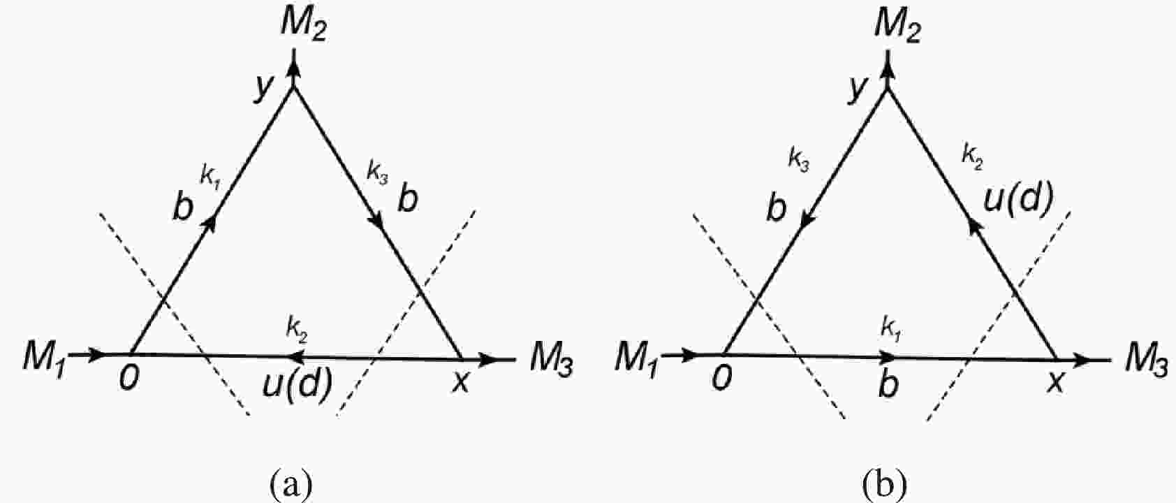
$ s=p^{2} $ ,$ u=p'^{2} $ , and$ q=p-p' $ . The QCD spectral density$ \rho(s,u,q^{2}) $ can be obtained by Cutkosky's rules [49] (see Fig. 1), the calculation for which is detailed in Ref. [29]. Moreover, we consider the contributions of$ \langle\overline{q}q\rangle $ ,$ \langle\overline{q}g_{s}\sigma Gq\rangle $ , and$ \langle\overline{q}q\rangle\langle g_{s}^{2}G^{2}\rangle $ . The Feynman diagrams for all of these condensate terms can be classified into two groups, as illustrated in Figs. 2 and 3.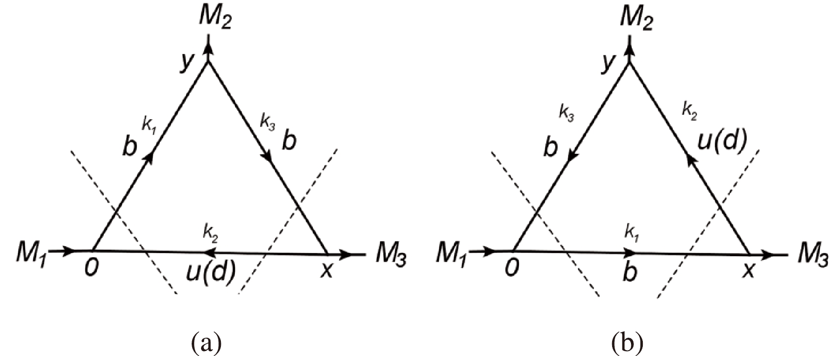
Figure 1. Perturbative contributions for
$ \Upsilon(\eta_{b}) $ (a) and$ B(B^{*}) $ (b) off-shell. The dashed lines denote the Cutkosky cuts.
Figure 2. Contributions of the non-perturbative parts for
$ \Upsilon(\eta_{b}) $ off-shell.
Figure 3. Contributions of the non-perturbative parts for
$ B(B^{*}) $ off-shell.We take the change in variables
$ p^{2}\to-P^{2} $ ,$ p'^{2}\to -P'^{2} $ , and$ q^{2}\to-Q^{2} $ and perform double Borel transformation on both the phenomenological and QCD sides. The variables$ P^{2} $ and$ P'^{2} $ are replaced by$ T_{1}^{2} $ and$ T_{2}^{2} $ , respectively, where$ T_{1} $ and$ T_{2} $ are called the Borel parameters. In this article, we take$ T^{2}=T_{1}^{2} $ and$ T_{2}^{2}=kT_{1}^{2}=kT^{2} $ , where k is a constant related to meson mass, with different values for different vertices, as presented in Table 2. Finally, the sum rules for the coupling constants can be obtained by matching the phenomenological and QCD sides according to the quark-hadron duality. The momentum dependent strong coupling constant can be written asVertices off-shell k E $ BB\Upsilon $ 

$\Upsilon $ 

$ 1 $ 

$ \dfrac{f_{B}^{2}m_{B}^{4}f_{\Upsilon}m_{\Upsilon}}{m_{b}^{2}} $ 

B $ \dfrac{m_{\Upsilon}^{2}}{m_{B^{*}}^{2}} $ 

$ \dfrac{2f_{B}^{2}m_{B}^{4}f_{\Upsilon}m_{\Upsilon}}{m_{b}^{2}} $ 

$ BB^{*}\Upsilon $ 

$\Upsilon $ 

$ \dfrac{m_{B^{*}}^{2}}{m_{B}^{2}} $ 

$ -\dfrac{f_{B}m_{B}^{2}f_{B^{*}}m_{B^{*}}f_{\Upsilon}m_{\Upsilon}}{m_{b}} $ 

B $ \dfrac{m_{\Upsilon}^{2}}{m_{B^{*}}^{2}} $ 

$ B^{*} $ 

$ \dfrac{m_{\Upsilon}^{2}}{m_{B}^{2}} $ 

$ B^{*}B^{*}\Upsilon $ 

$\Upsilon $ 

$ 1 $ 

$ -f_{B^{*}}^{2}m_{B^{*}}^{2}f_{\Upsilon}m_{\Upsilon} $ 

$ B^{*} $ 

$ \dfrac{m_{\Upsilon}^{2}}{m_{B}^{2}} $ 

$ -2f_{B^{*}}^{2}m_{B^{*}}^{2}f_{\Upsilon}m_{\Upsilon} $ 

$ BB^{*}\eta_{b} $ 

$ \eta_{b} $ 

$ \dfrac{m_{B^{*}}^{2}}{m_{B}^{2}} $ 

$ -\dfrac{f_{B}m_{B}^{2}f_{B^{*}}m_{B^{*}}f_{\eta_{b}}m_{\eta_{b}}^{2}}{m_{b}^{2}} $ 

B $ \dfrac{m_{\eta_{b}}^{2}}{m_{B^{*}}^{2}} $ 

$ B^{*} $ 

$ \dfrac{m_{\eta_{b}}^{2}}{m_{B}^{2}} $ 

$ \dfrac{f_{B}m_{B}^{2}f_{B^{*}}m_{B^{*}}f_{\eta_{b}}m_{\eta_{b}}^{2}(m_{\eta_{b}}^{2}+m_{B^{*}}^{2}-m_{B}^{2})}{2m_{b}^{2}m_{B^{*}}^{2}} $ 

$ B^{*}B^{*}\eta_{b} $ 

$ \eta_{b} $ 

$ 1 $ 

$ -\dfrac{f_{B^{*}}^{2}m_{B^{*}}^{2}f_{\eta_{b}}m_{\eta_{b}}^{2}}{2m_{b}^{2}} $ 

$ B^{*} $ 

$ \dfrac{m_{\eta_{b}}^{2}}{m_{B^{*}}^{2}} $ 

Table 2. Parameters k and E for different vertices and off-shell cases.
$ g({Q^2}) = \frac{{ - \int\limits_{{s_1}}^{{s_0}} {\int\limits_{{u_1}}^{{u_0}} {\rho (s,u,{Q^2}){{\rm e}^{ - s/{T^2}}}{{\rm e}^{ - u/k{T^2}}}} {\rm d}s{\rm d}u + \mathscr B\mathscr B[{{\Pi }^{\mathrm{non - pert}}}]} }}{{\dfrac{E}{{(m_{M_2}^2 + {Q^2})}}{{\rm e}^{ - m_{M_1}^2/{T^2}}}{{\rm e}^{ - m_{M_3}^2/k{T^2}}}}} $

(18) where
$ \mathscr{BB} $ stands for the double Borel transformation, and E is a factor related to meson masses and decay constants (see Table 2). From this equation, we can also see that the threshold parameters$ s_{0} $ and$ u_{0} $ in the dispersion integral are introduced. These parameters are used to eliminate the contributions of higher resonances and continuum states in Eq. (3). They commonly fulfill the relations$ m_{\mathrm{i}}^{2}<s_{0}<m'^{2}_{\mathrm{i}} $ and$ m_{\mathrm{o}}^{2}<u_{0}<m'^{2}_{\mathrm{o}} $ , where subscripts i and o represent incoming and outcoming mesons, respectively. m and$ m' $ are the masses of the ground and first excited states of the mesons. Generally,$ m'=m+\Delta $ , where Δ is taken as a value in the range of$ 0.4 \sim 0.6 $ GeV [24].The strong coupling constant in Eq. (18) is momentum dependent, similar to the run coupling constant
$ \alpha_{s} $ . To obtain the final results of the strong coupling constant, it is necessary to extrapolate the results obtained from Eq. (18) into time-like regions$ (Q^{2}<0) $ . This process is realized by fitting$ g(Q^{2}) $ into appropriate analytical functions and setting ($ Q^2=-m_{\mathrm{on-shell}}^{2} $ ). -
All input parameters are taken as the standard values such as the hadronic masses and decay constants
$ m_{B}=5.28 $ GeV [50],$ m_{B^{*}}=5.33 $ GeV [50],$ m_{\Upsilon}= 9.46 $ GeV [50],$ m_{\eta_{b}}=9.399 $ GeV [50],$ f_{B}=0.192\pm0.013 $ GeV [51],$ f_{B^{*}}=0.213\pm0.018 $ GeV [51],$ f_{\Upsilon}=0.7 $ GeV [50], and$ f_{\eta_{b}}=0.667\pm0.007 $ GeV [52]. The vacuum condensates are also adopted as the standard values, which are$ \langle\overline{q}q\rangle=-(0.23\pm0.01)^{3} $ GeV$ ^{3} $ [50],$\langle\overline{q}g_{s}\sigma Gq\rangle= m_{0}^{2}\langle\overline{q}q\rangle$ [50],$ m_{0}^{2}=0.8\pm0.1 $ GeV$ ^2 $ [53−55],$\langle g_{s}^{2}G^{2}\rangle= 0.88\pm0.15$ GeV$ ^{4} $ [53−55], and$ \langle f^{3}G^{3}\rangle=(8.8\pm5.5) $ GeV$ ^{2}\langle g_{s}^{2}G^{2}\rangle $ [53−55]. The$ \mathrm{\overline{MS}} $ mass of light and heavy quarks is adopted from the Particle Data Group [50], where$ m_{u(d)}(\mu=1 \mathrm{GeV})= 0.006\pm 0.001 $ GeV and$ m_{b}(m_{b})=4.18\pm0.03 $ GeV. In principle, both the vacuum condensates and the$ \mathrm{\overline{MS}} $ masses of light and heavy quarks are energy-scale dependent. For the B meson, the influences of vacuum condensates and the masses of light quarks are smaller than that of the bottom quark. More specifically, the mass of the bottom quark has a significant influence on the results, and its energy-scale dependency should be considered and discussed. The energy-scale dependent$ \mathrm{\overline{MS}} $ mass of bottom quark can be expressed as follows according to the re-normalization group equation,$ \begin{aligned}[b] {m_b}(\mu ) =& {m_b}({m_b}){\left[\frac{{{\alpha _s}(\mu )}}{{{\alpha _s}({m_b})}}\right]^{\frac{{12}}{{33 - 2{n_f}}}}}\\ {\alpha _s}(\mu ) =& \frac{1}{{{b_0}t}}\left[1 - \frac{{{b_1}}}{{b_0^2}}\frac{{\log t}}{t} \right.\\ &\left.+ \frac{{b_1^2({{\log }^2}t - \log t - 1) + {b_0}{b_2}}}{{b_0^4{t^2}}}\right], \end{aligned} $

(19) where
$t=\mathrm{log}\dfrac{\mu^2}{\Lambda_{\rm QCD}^2}$ ;$ b_{0}=\dfrac{33-2n_{f}}{12\pi} $ ;$ b_{1}=\dfrac{153-19n_{f}}{24\pi^{2}} $ ;$b_{2}=({2857-\dfrac{5033}{9}n_{f}+\dfrac{325}{27}n_{f}^{2}})/({128\pi^{3}})$ ; and$\Lambda_{\rm QCD}=210$ MeV, 292 MeV, and 332 MeV for the flavors$ n_{f}=5, 4 $ , and 3, respectively [50]. In the framework of QCDSR, the final results should be obtained by selecting an appropriate energy-scale. In some similar research, the masses of heavy quarks in the energy-scale$ \mu=m_{Q} $ were employed to obtain the coupling constants [24, 28]. In the present study, the mass of bottom quark in the energy-scale$ \mu=m_{b} $ is also used to obtain the strong coupling constants [50]. The dependence of the strong coupling constants on energy-scales will be discussed at the end of this section.According to Eq. (18), the strong coupling constant is a function of some input parameters such as the Borel parameter
$ T^{2} $ , continuum thresholds$ s_{0} $ and$ u_{0} $ , and square momentum$ Q^{2} $ . The Borel parameter$ T^{2} $ is determined by two conditions, which are the pole dominance and convergence of OPE. To analyze the pole contribution, we first write$ \begin{aligned}[b] \Pi^{\mathrm{OPE}}_{\mathrm{pole}}(T^{2})=-\int_{s_{1}}^{s_{0}}\int_{u_{1}}^{u_{0}}\rho^{\mathrm{OPE}}(s,u,Q^2){\rm e}^{-\frac{s}{T^{2}}}{\rm e}^{-\frac{u}{kT^{2}}}{\rm d}s{\rm d}u \\ \Pi^{\mathrm{OPE}}_{\mathrm{cont}}(T^{2})=-\int_{s_{0}}^{\infty}\int_{u_{0}}^{\infty}\rho^{\mathrm{OPE}}(s,u,Q^2){\rm e}^{-\frac{s}{T^{2}}}{\rm e}^{-\frac{u}{kT^{2}}}{\rm d}s{\rm d}u . \end{aligned} $

(20) Meanwhile, the pole and continuum contributions are defined as [24]
$ \begin{aligned}[b] \mathrm{Pole}=&\frac{\Pi^{\mathrm{OPE}}_{\mathrm{pole}}(T^{2})}{\Pi^{\mathrm{OPE}}_{\mathrm{pole}}(T^{2})+\Pi^{\mathrm{OPE}}_{\mathrm{cont}}(T^{2})} \\ \mathrm{Continuum}=&\frac{\Pi^{\mathrm{OPE}}_{\mathrm{cont}}(T^{2})}{\Pi^{\mathrm{OPE}}_{\mathrm{pole}}(T^{2})+\Pi^{\mathrm{OPE}}_{\mathrm{cont}}(T^{2})}. \end{aligned} $

(21) In addition, the continuum threshold parameters
$ s_{0} $ and$ u_{0} $ are employed to include the pole contribution and suppress the contribution of higher resonances and continuum states. Their values commonly satisfy the relations$s_{0}=(m_{i}+\Delta_{i})^{2}$ and$u_{0}=(m_{o}+\Delta_{o})^{2}$ , where the subscripts i and o represent the incoming and outcoming mesons, respectively. The values of$\Delta_{i}$ and$\Delta_{o}$ should be smaller than the experimental value of the distance between the ground and first excited states. In general,$\Delta_{i}$ and$\Delta_{o}$ are considered as 0.5 GeV.Taking the strong coupling constant
$ g_{BB\Upsilon}^{\Upsilon} $ as an example, we introduce the method of selection for the above parameters. Fixing$ Q^{2}=3 $ GeV$ ^{2} $ in Eq. (18), we first plot the strong coupling constant$ g_{BB\Upsilon}^{\Upsilon} $ for the Borel parameter$ T^{2} $ at different values of$ s_{0} $ and$ u_{0} $ ; this dependence is shown in Fig. 4, indicating that the results have good stability when$ s_{0} $ and$ u_{0} $ are 31.14$ \sim $ 35.76 GeV$ ^{2} $ (the corresponding values of$\Delta_{i}$ and$\Delta_{o}$ are 0.3$ \sim $ 0.7 GeV). The pole and continuum contributions with variation of the Borel parameter$ T^{2} $ are depicted in Fig. 5. In can be seen from this figure that the condition of pole dominance ($ \geq $ 40%) is satisfied in the range 17 GeV$ ^{2} $ $ \leq T^{2}\leq $ 19 GeV$ ^{2} $ . The contributions of the total, perturbative, and all vacuum condensate terms for vertex$ BB\Upsilon $ are explicitly shown in Figs. 6 (a) and (b). These results demonstrate good stability with variation of Borel parameter$ T^{2} $ in the range 17 GeV$ ^{2} $ $ \leq T^{2}\leq $ 19 GeV$ ^{2} $ , indicating that the condition of OPE convergence is also satisfied. This flat region (17 GeV$ ^{2} $ $ \leq T^{2}\leq $ 19 GeV$ ^{2} $ ) is usually called the "Borel Window" and is used to extract the final results. According to a similar analysis with$ g_{BB\Upsilon}^{\Upsilon} $ , the Borel Window for other strong vertices are also determined with$\Delta_{i}=\Delta_{o}=0.5$ GeV, as shown in Fig. 6.
Figure 4. (color online) Strong coupling constants
$ g_{BB\Upsilon}^{\Upsilon} $ for the Borel parameter$ T^{2} $ at different values of$ s_{0} $ (a) and$ u_{0} $ (b).
Figure 5. (color online) Pole and continuum contributions with variation of the Borel parameter
$ T^{2} $ for the vertex$ BB\Upsilon $ in the Υ off-shell case.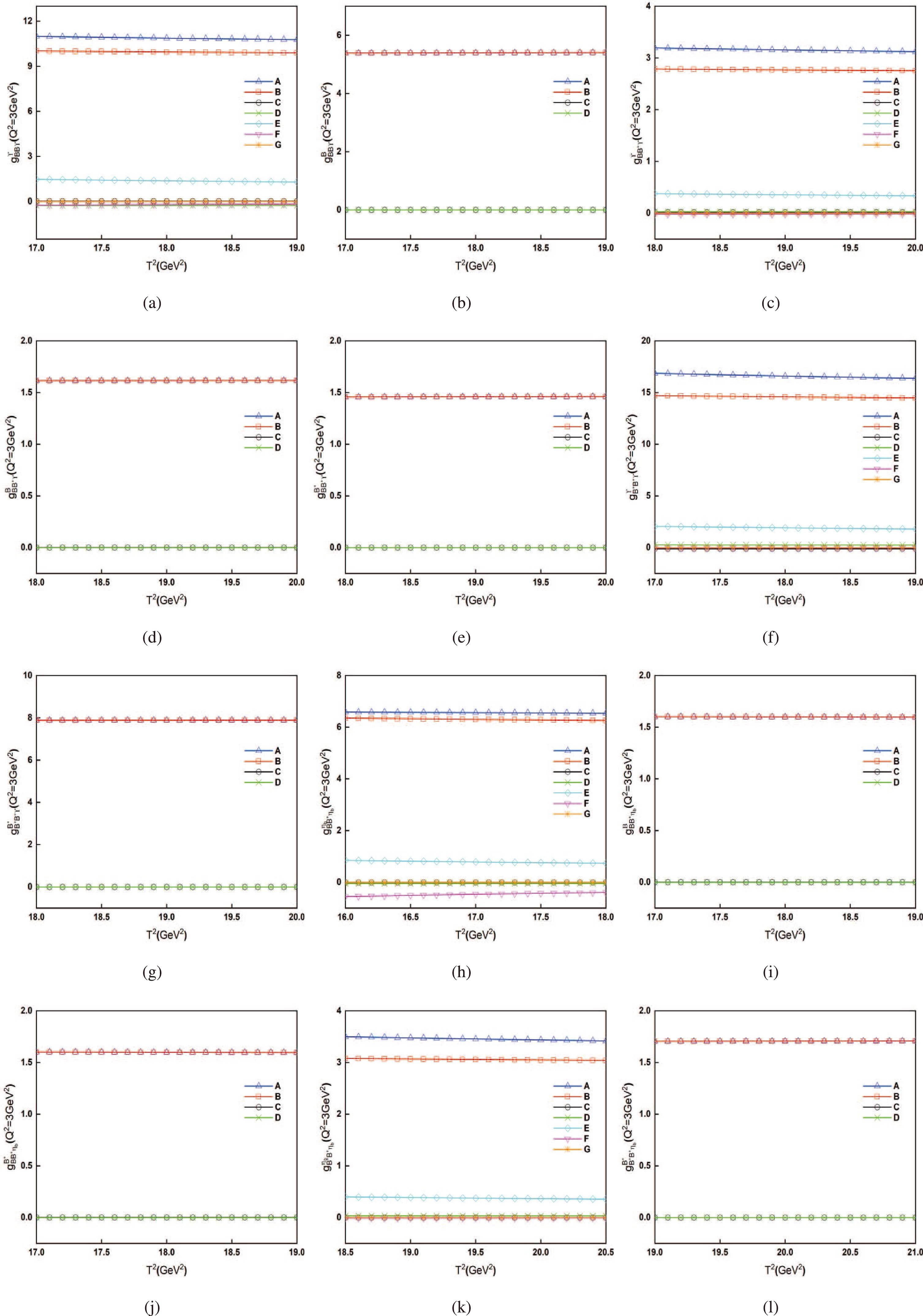
Figure 6. (color online) Contributions of different vacuum condensate terms with variations of the Borel parameter
$ T^{2} $ for$ BB\Upsilon $ (a−b),$ BB^{*}\Upsilon $ (c−e),$ B^{*}B^{*}\Upsilon $ (f−g),$ BB^{*}\eta_{b} $ (h−j), and$ B^{*}B^{*}\eta_{b} $ (k−l), where A-G denote the total, perturbative,$ \langle g_{s}^{2}G^{2}\rangle, \langle f^{3}G^{3}\rangle,\langle\overline{q}q\rangle, \langle\overline{q}g_{s}\sigma G q\rangle $ , and$ \langle\overline{q}q\rangle\langle g_{s}^{2}G^{2}\rangle $ contributions.Considering different values of
$ Q^{2} $ , the momentum dependent strong coupling constant$ g(Q^{2}) $ can be obtained with the values of$ Q^{2} $ being taken as 3$ \sim $ 28 GeV$ ^{2} $ uniformly. The on-shell values of these coupling constants can be obtained by extrapolating the results ($ g(Q^{2}) $ ) to the time-like regions ($ Q^{2}<0 $ ). This process is implemented by fitting$ g(Q^{2}) $ with appropriate functions and setting the intermediate meson on-shell ($ Q^{2}=-m^{2}_{\mathrm{on-shell}} $ ). To choose appropriate fitting functions, two conditions should be satisfied: first, the strong coupling constants should be well fitted in the space-like regions ($ Q^{2}>0 $ ); second, the values of the strong coupling constants in deep time-like regions should converge. In addition, the on-shell values for the same vertex in different off-shell cases should be as close to each other as possible. Considering the above requirements, the uncertainties of the fitting function selection can be greatly reduced. Taking the strong coupling constant$ g_{BB\Upsilon} $ as an example,$ g(Q^{2}) $ can be fitted into two functions with$\Upsilon $ and B being off-shell cases, expressed as$ \begin{aligned}[b] C1:\quad &g_{BB\Upsilon }^\Upsilon ({Q^2}) = 11.43{{\rm e}^{ - 0.013{Q^2}}}\\ &g_{BB\Upsilon }^B({Q^2}) = 7.99{{\rm e}^{ - 0.062{Q^2}}} - 1.20\\ C2:\quad &g_{BB\Upsilon }^\Upsilon ({Q^2}) = 11.78{{\rm e}^{0.02{Q^2}}} - 0.45{Q^2}\\ &g_{BB\Upsilon }^B({Q^2}) = 6.84{{\rm e}^{ - 0.072{Q^2}}} - 0.03{Q^2}. \end{aligned} $

(22) Their fitting curves are shown in Fig. 7, where we can see that both the fitting curves
$ C1 $ and$ C2 $ are well fitted in the space-like regions for$\Upsilon $ and B off-shell cases, and the on-shell values are well convergent. For the case of$ g_{BB\Upsilon}^{\Upsilon} $ , the curve$ C1 $ (the blue solid line) is better fitted in the space-like regions than curve$ C2 $ (the blue dashed line). Thus, fitting function$ C1 $ is selected for$ g_{BB\Upsilon} $ in the Υ off-shell case. For the B off-shell case, the curves$ C1 $ and$ C2 $ almost overlap each other in the space-like regions (the black solid and dashed lines). As stated above, the on-shell values for same vertex in different off-shell cases should be close to each other. We can see that curve$ C1 $ is more appropriate for this condition. Thus,$ C1 $ is selected to fit$ g_{BB\Upsilon} $ in the B off-shell case.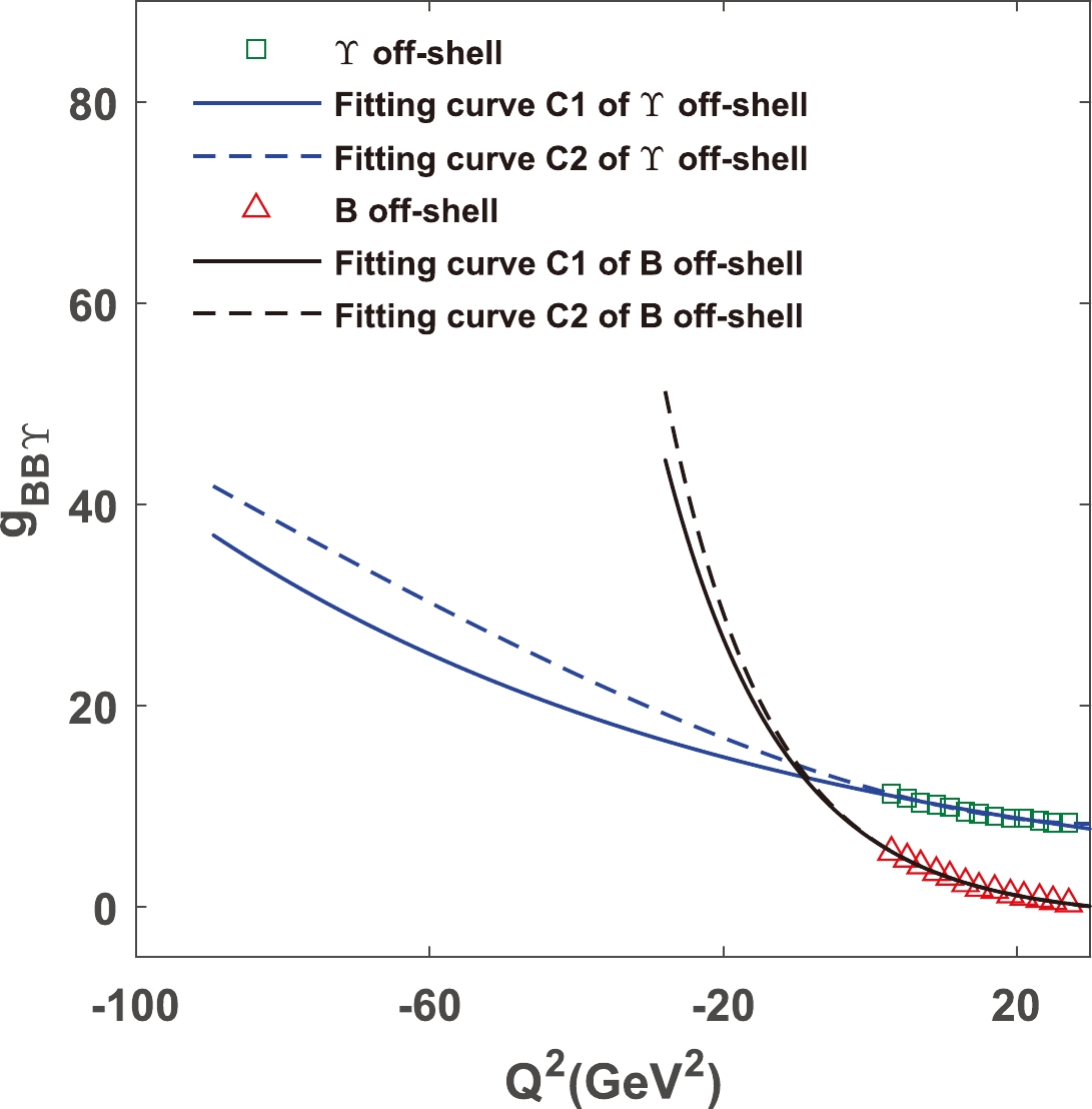
Figure 7. (color online) Fitting curves of the coupling constants for vertex
$ BB\Upsilon $ in$\Upsilon $ and B off-shell cases.We know that the mass of the bottom quark is strongly energy-scale dependent, which also influences the final results obtained by QCDSR. Taking the coupling constant
$ g_{BB\Upsilon}^{\Upsilon}(Q^{2}) $ as an example, we plot this dependence in Fig. 8 , for which the values are fitted by the$ C1 $ function. From this figure, we can see that the results are indeed strongly dependent on the energy-scale μ. Actually, it is difficult to determine the appropriate energy-scale when calculating the coupling constants with QCDSR or LCSR. In some previous studies, similar calculations were carried out by QCDSR and LCSR with different energy-scales of heavy quarks [45, 47]. In the present study, the strong coupling constants are obtained with the mass of the bottom quark in the energy-scale$ \mu=m_{b} $ [50].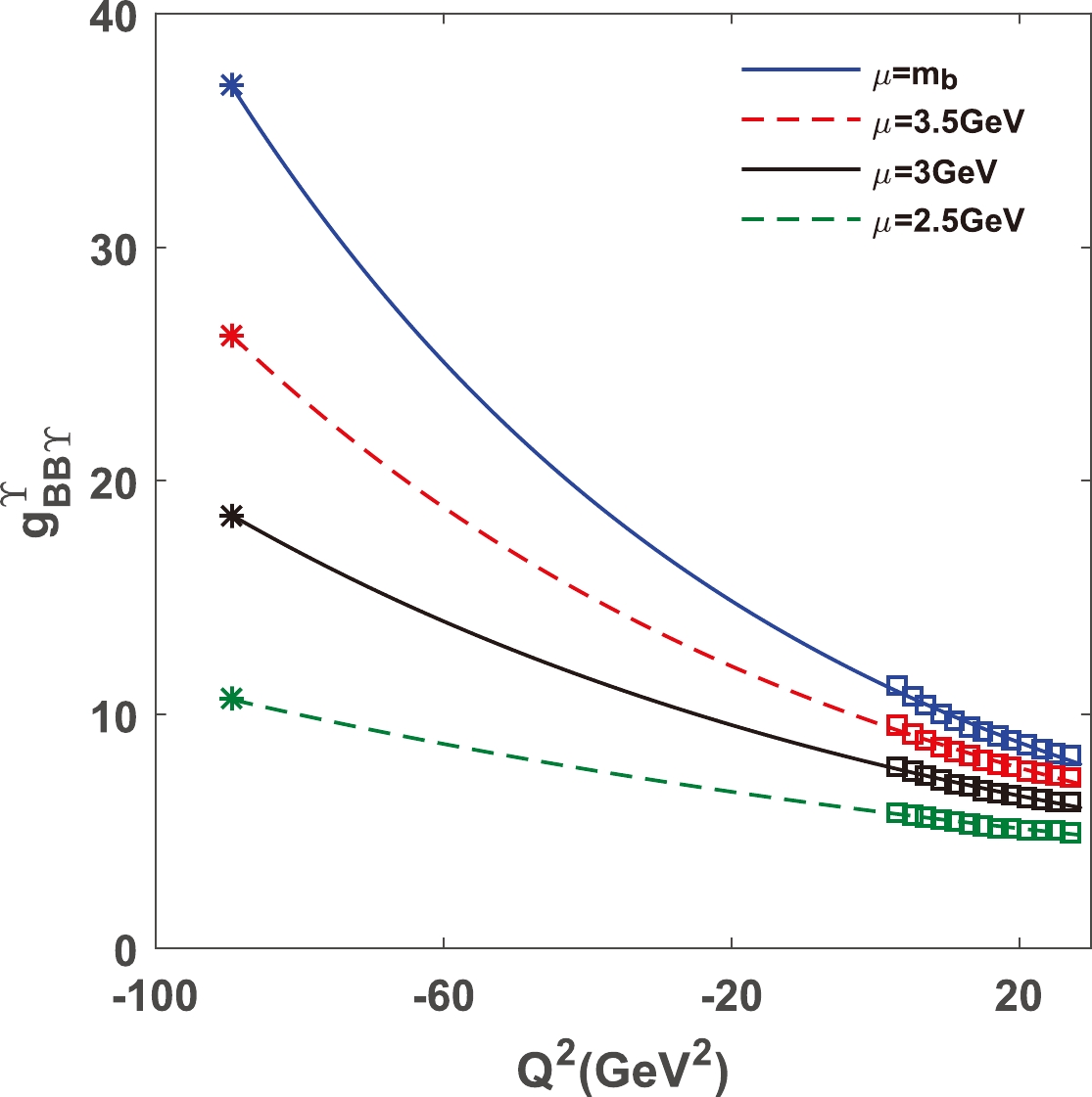
Figure 8. (color online) Dependence of strong coupling constant
$ g_{BB\Upsilon}^{\Upsilon} $ on bottom quark mass with different energy-scales.Finally, the momentum dependent strong coupling constants can be uniformly fitted into the following analytical function:
$ \begin{array}{*{20}{l}} g(Q^{2})=F{\rm e}^{-GQ^{2}}+H, \end{array} $

(23) where the values of parameters F, G, and H are as listed in Table 3. The fitting diagrams of strong coupling constants for each vertex are shown in Fig. 9.
Vertex off-shell F G H $ g(Q^{2}=-m_{\mathrm{on-shell}}^{2}) $ 

$ BB\Upsilon $ 

$\Upsilon $ 

$ 11.43 $ 

$ 0.013 $ 

$ 0 $ 

$ 36.92^{+3.51}_{-3.80} $ 

B $ 7.99 $ 

$ 0.062 $ 

$ -1.20 $ 

$ 44.42^{+11.59}_{-4.60} $ 

$ BB^{*}\Upsilon $ 

$\Upsilon $ 

$ 3.17 $ 

$ 0.014 $ 

$ 0 $ 

$ 11.35^{+1.01}_{-1.11} $ GeV−1

B $ 2.39 $ 

$ 0.057 $ 

$ -0.39 $ 

$ 11.36^{+2.31}_{-0.88} $ GeV−1

$ B^{*} $ 

$ 2.17 $ 

$ 0.061 $ 

$ -0.33 $ 

$ 12.04^{+3.24}_{-1.29} $ GeV−1

$ B^{*}B^{*}\Upsilon $ 

$\Upsilon $ 

$ 16.24 $ 

$ 0.014 $ 

$ 0 $ 

$ 55.10^{+4.67}_{-5.07} $ 

$ B^{*} $ 

$ 11.63 $ 

$ 0.058 $ 

$ -1.84 $ 

$ 58.93^{+5.98}_{-5.55} $ 

$ BB^{*}\eta_{b} $ 

$ \eta_{b} $ 

$ 6.72 $ 

$ 0.015 $ 

$ 0 $ 

$ 25.52^{+1.84}_{-2.06} $ 

B $ 4.71 $ 

$ 0.064 $ 

$ -0.66 $ 

$ 27.31^{+6.35}_{-2.51} $ 

$ B^{*} $ 

$ 2.39 $ 

$ 0.071 $ 

$ -0.28 $ 

$ 17.34^{+6.03}_{-2.34} $ 

$ B^{*}B^{*}\eta_{b} $ 

$ \eta_{b} $ 

$ 3.48 $ 

$ 0.014 $ 

$ 0 $ 

$ 11.97^{+1.05}_{-1.41} $ GeV−1

$ B^{*} $ 

$ 2.46 $ 

$ 0.060 $ 

$ -0.39 $ 

$ 13.00^{+3.20}_{-1.27} $ GeV−1

Table 3. Fitting parameters in Eq. (23) and the strong coupling constants for different vertices and off-shell cases.
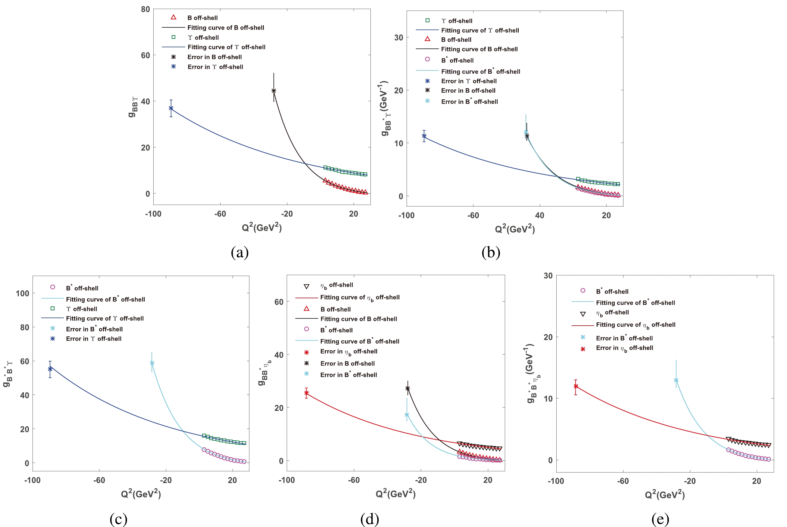
Figure 9. (color online) Fitting curves of coupling constants for vertices
$ BB\Upsilon $ (a),$ BB^{*}\Upsilon $ (b),$ B^{*}B^{*}\Upsilon $ (c),$ BB^{*}\eta_{b} $ (d), and$ B^{*}B^{*}\eta_{b} $ (e). In these figures, all possible off-shell cases are considered.Then,
$ g(Q^{2}) $ is extrapolated to the time-like regions$ (Q^{2}<0) $ by Eq. (23), and the on-shell condition is satisfied by setting$ Q^{2}=-m_{\mathrm{on-shell}}^{2} $ . The on-shell values of strong coupling constants for different off-shell cases are obtained and listed in the last column of Table 3.For each vertex, the on-shell values of coupling constants for different off-shell cases should be equal to each other. For vertex
$ BB^{*}\Upsilon $ as an example, the central values for different off-shell cases are$ g_{BB^{*}\Upsilon}^{\Upsilon}=11.35 $ GeV$ ^{-1} $ ,$ g_{BB^{*}\Upsilon}^{B}=11.36 $ GeV$ ^{-1} $ , and$ g_{BB^{*}\Upsilon}^{B^{*}}=12.04 $ GeV$ ^{-1} $ , which are consistent with each other. Thus, it is reasonable to determine the final values of the strong coupling constants by taking their average values. Finally, the results of the strong coupling constants for different strong vertices are determined as$ \begin{aligned}[b] g_{BB\Upsilon}=&40.67^{+7.55}_{-4.20} \\ g_{BB^{*}\Upsilon}=&11.58^{+2.19}_{-1.09} \mathrm{GeV}^{-1} \\ g_{B^{*}B^{*}\Upsilon}=&57.02^{+5.32}_{-5.31} \\ g_{BB^{*}\eta_{b}}=&23.39^{+4.74}_{-2.30} \\ g_{B^{*}B^{*}\eta_{b}}=&12.49^{+2.12}_{-1.35} \mathrm{GeV}^{-1} .\end{aligned} $

(24) -
In this work, we systematically analyzed the strong vertices
$ BB\Upsilon $ ,$ BB^{*}\Upsilon $ ,$ B^{*}B^{*}\Upsilon $ ,$ BB^{*}\eta_{b} $ , and$ B^{*}B^{*}\eta_{b} $ using the QCD sum rules, considering all off-shell cases for each vertex. Under this physical sketch, the momentum dependent coupling constants were first obtained in space-like ($ Q^{2}>0 $ ) regions and then fitted into appropriate analytical functions. By extrapolating these functions to time-like ($ Q^{2}<0 $ ) regions and taking$ Q^{2}=-m^{2}_{\mathrm{on-shell}} $ , we obtained the strong on-shell coupling constants. For each vertex, we considered the average value of the strong on-shell coupling constants for all off-shell cases as the final result. These coupling constants are valuable in describing the dynamical behaviors of hadrons. For example, these coupling constants are important input parameters to analyze the final-state interactions in heavy quarkonium decays or to calculate the absorption cross sections for understanding heavy quarkonium absorptions in hadronic matter.
Strong vertices of bottom mesons B and B* and bottomonia ${\Upsilon }$ , ηb
- Received Date: 2023-08-14
- Available Online: 2024-01-15
Abstract: In this study, the strong coupling constants of vertices


 DownLoad: