


 Abstract
 HTML
HTML Reference
 Related
 PDF
PDF


-
The
$ X(6900) $ peak observed by the LHCb Collaboration in the di-$ J/\psi $ invariant mass spectrum [1, 2], and later in the$ J\psi\psi(3686) $ invariant mass spectrum [3], has stimulated many discussions of theoretical aspects (see for example Ref. [4] for an incomplete list of references). Moreover,$ X(6900) $ is close to the threshold of$ J/\psi \psi(3770) $ ,$ J/\psi \psi_2(3823) $ ,$ J/\psi $ $ \psi_3(3842) $ , and$ \chi_{c0} \chi_{c1} $ , whereas$ X(7200) $ is close to the threshold of$ J/\psi \psi(4160) $ and$ \chi_{c0} $ $ \chi_{c1}(3872) $ ). Inspired by this, Ref. [5] studied the properties of$ X(6900) $ and$ X(7200) $ by assuming the$ X(6900) $ coupling to$ J/\psi J/\psi $ ,$ J/\psi\psi(3770) $ ,$ J/\psi \psi_2(3823) $ ,$ J/\psi \psi_3(3842) $ , and$ \chi_{c0}\chi_{c1} $ channels and the$ X(7200) $ coupling to$ J/\psi J/\psi $ ,$ J/\psi\psi(4160) $ , and$ \chi_{c0}\chi_{c1}(3872) $ channels. For the S-wave$ J/\psi J/\psi $ coupling, the pole counting rule (PCR) [6], which has been applied to the studies of "$ XYZ $ " physics in Refs. [7−10], was employed to analyze the nature of the two structures. It was found that the di-$ J/\psi $ data alone are not sufficient to judge the intrinsic properties of the two states. It was also pointed out that$ X(6900) $ is unlikely a molecule of$ J/\psi\,\psi(3686) $ [5], a conclusion drawn before the discovery of Ref. [3]. More recently, Refs. [4, 11, 12] investigated$ X(6900) $ using a combined analysis of di-$ J/\psi $ and$ J/\psi\psi(3686) $ data and concluded that$ X(6900) $ cannot be a$ J/\psi\psi(3686) $ molecule.Nevertheless, as already stressed in Ref. [4], even though
$ X(6900) $ is very unlikely a molecule of$ J/\psi\psi(3686) $ , this does not mean that it has to be an "elementary state" (i.e., a compact$ \bar c\bar ccc $ tetraquark state). It was pointed out that it is possible that$ X(6900) $ be a molecular state composed of other particles, such as$ J/\psi\psi(3770) $ , which form thresholds closer to$ X(6900) $ if the channel coupling is sufficiently large1 .This note will discuss a possible mechanism for the enhancement of the
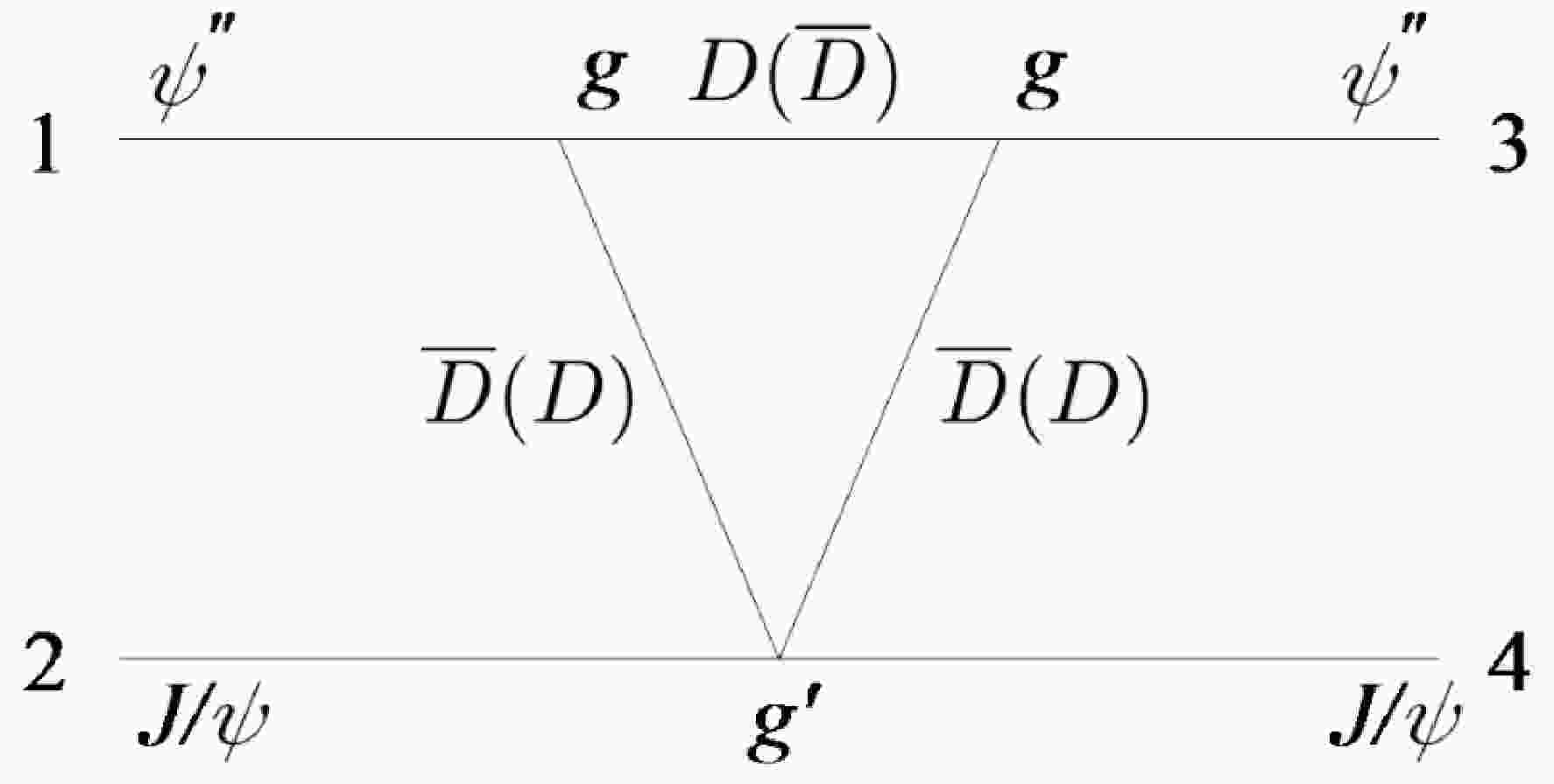
$ J/\psi\psi(3770) $ channel coupling. The$ D\bar D $ (or$ D^*\bar D^* $ ) component inside$ \psi(3770) $ may play an important role, so far ignored in the literature, in explaining the$ X(6900) $ resonant peak through the anomalous threshold emerged from the triangle diagram generated by the D ($ D^* $ ) loop, as depicted in Fig. 1.
Figure 1.
$ D\bar D $ triangle diagram in the$ J/\psi \psi'' $ scattering process.Noticing that
$ \psi(3770) $ or$ \psi'' $ couples dominantly to$ D\bar D $ , we start from the Feynman diagram as depicted in Fig. 1 by assuming that it contributes to$ J/\psi\psi'' $ elastic scatterings near the$ J/\psi \psi'' $ threshold2 . Assuming an interaction Lagrangian3 $ \begin{aligned}[b] \mathcal{L} =& -{\rm i}g(D^0\partial_\mu\bar{D}^0 - \bar{D}^0\partial_\mu D^0) \psi''^\mu -{\rm i}g (D^+\partial_\mu D^- - D^-\partial_\mu D^+) \psi''^\mu\\ &+ g' D^0\bar{D}^0 J/\psi^\mu J/\psi_\mu+ g' D^+D^- J/\psi^\mu J/\psi_\mu\ , \end{aligned} $

(1) after performing the momentum integration, the amplitude as depicted by Fig. 1 is
$ \begin{aligned}[b] {\rm i}\mathcal{M} =& (-16 g^2 g') \; (\epsilon_2 \cdot \epsilon_4) \; \epsilon_1^\mu \epsilon_3^\nu \int {\rm d}^Dk\\&\times \frac{k_\mu k_\nu}{((k-p_1)^2-m_D^2)((k-p_3)^2-m_D^2)(k^2-m_D^2)}\\ \equiv& (-16 g^2 g') \; (\epsilon_2 \cdot \epsilon_4) \; \epsilon_1^\mu \epsilon_3^\nu \; \mathcal{A}_{\mu\nu} \end{aligned} $

(2) where
$ \begin{aligned}[b] \mathcal{A}^{\mu\nu}& =\frac{-{\rm i}}{16\pi^2}\int_0^1 {\rm d}x\int_0^{1-x}{\rm d}y \; \left\{\frac{p_3^\mu p_1^\nu \; xy}{\Delta} - \frac{g^{\mu\nu}}{4} \Gamma(\epsilon) \frac{1}{\Delta^\epsilon} \right\}\\ & \equiv \frac{-{\rm i}}{16\pi^2} \left\{ p_3^\mu p_1^\nu\; \mathcal{B} + \int_0^1 {\rm d}x\int_0^{1-x}{\rm d}y \left(- \frac{g^{\mu\nu}}{4} \Gamma(\epsilon) \frac{1}{\Delta^\epsilon} \right)\right\}\ , \end{aligned} $

(3) and
$ \begin{aligned}[b] \mathcal{B}(t) = &\int_0^1 {\rm d}x \frac{x}{2M^2} \Bigg( 2(M^2(1-2x)+tx)\\&\times\frac{\mathrm{ArcTan}\left(\dfrac{M^2-tx}{\Lambda(t,x)}\right)-\mathrm{ArcTan}\left(\dfrac{M^2(2x-1)-tx}{\Lambda(t,x)}\right)}{\Lambda(t,x)} \\ &+\left. \ln \frac{m^2+t(x-1)x}{m^2+M^2(x-1)x}\right)\ . \end{aligned} $

(4) Here,
$ \Lambda(t, x)= \sqrt{ 4 m^2 M^2 - M^4 + 4 M^2 t x^2 - 2 M^2 t x - t^2 x^2} $ ,$\Delta = M^2(x^2+y^2)+(2M^2-t)xy-M^2(x+y)+m^2$ , and$ \Gamma(\epsilon) \dfrac{1}{\Delta^\epsilon} = \dfrac{1}{\epsilon} - \ln \Delta - \gamma + \ln 4\pi + \mathcal{O}(\epsilon) $ . On the right hand side of Eq. (3), only the$ \mathcal{B} $ term will be considered since the rest will be absorbed by the contact interactions to be introduced latter. M is the mass of$ \psi(3770) $ , and m is the mass of$ D(\bar D) $ . Parameter g is the coupling strength of the$ \psi'' \;\; D\bar D $ three point vertex, and$ g' $ is the coupling strength of the$ J/\psi J/\psi D\bar D $ four point vertex; {$ t=(p_2-p_4)^2 $ }. Parameter g can be determined by the$ \psi''\to D^0\bar{D}^0 $ decay process ,$ \begin{aligned}[b] {\rm i} \mathcal{M}_{\psi'' DD} =& {\rm i} \,g \,\epsilon(\psi'') \cdot [p(D^0)-p(\bar{D}^0)]\ ,\\ \Gamma =& \frac{1}{8\pi}\,|{\rm i} \mathcal{M}_{\psi'' DD}|^2\,\frac{q(DD)}{M_{\psi''}^2} = \frac{1}{6 \pi} \, g^2 \, \frac{q(DD)^3}{M_{\psi''}^2}\ , \end{aligned} $

(5) where
$ q(DD) $ is the norm of the three-dimensional momentum of$ D^0 $ or$ \bar{D}^0 $ in the final state. The PDG value$ \Gamma_{\psi''\to D^0\bar{D}^0} \sim 27.2\times 52{\text%} \times10^{-3} $ [16] determines$ g \sim 12 $ 4 . Parameter$ g' $ is unknown and is left as a free parameter. The amplitude, Eq. (4), contains a rather complicated singularity structure, especially the well-known anomalous threshold, which was discovered by Mandelstam who used it to explain the looseness of the deuteron wave function [18]. The anomalous threshold is located at$ s_A = 4m^2-\frac{(M^2-2m^2 )^2 }{m^2}\ . $

(6) Considering the mass of the
$ \psi'' $ and$ D^0 $ mesons, one obtains$ s_A=-1.28 $ GeV$ ^2 $ (for the$ D^+ $ loop, –0.98 GeV$ ^2 $ ). Numerically, function$ \cal{B} $ is plotted in Fig. 2(a), where one clearly sees the anomalous threshold beside the normal one at$ t=4m^2 $ . Note that if$ M^2 $ is smaller than$ 2m^2 $ , the anomalous branch point is located below the physical threshold, but on the second sheet. It touches the physical threshold$ 4m^2 $ and turns up to the physical sheet if the value of$ M^2 $ increases to$ 2m^2 $ . With a further increase in$ M^2 $ , the anomalous threshold moves towards the left on the real axis, passes the origin when$ M^2=4m^2 $ , and finally reaches the physical value, i.e., –1.28 GeV$ ^2 $ . The situation is depicted in Fig. 2(b). Note that$ s_A $ here is negative, contrary to what occurs with the deuteron, because the latter is a bound state with a normalizable wave function, whereas$ \psi'' $ is an unstable resonance.
Figure 2. (color online) Left: triangle diagram contribution (the y axis label is arbitrary). Right: the trajectory of the anomalous threshold with respect to the variation of
$ M^2 $ .To proceed, one needs to make the partial wave projection of
$ \mathcal{M} $ and obtain$ \begin{aligned}[b] T^J_{\mu_1\mu_2\mu_3\mu_4}(s)=&\frac{1}{32\pi}\frac{1}{2q^2(s)}\int^0_{-4q^2(s)}\,{\rm d}t\, d^J_{\mu\mu'}\\&\times\left(1+\frac{t}{2q^2(s)}\right)\mathcal{M}_{\mu_1\mu_2\mu_3\mu_4}(t)\ , \end{aligned} $

(7) where the channel momentum square reads
$q^2(s)= [s - (M - M_J)^2] [s - (M + M_J)^2]/4s$ ,$ M_J $ is the mass of$ J/\psi $ ,$ \mu_i $ denotes the corresponding helicity configuration, and$ \mu = \mu_1-\mu_2 $ ,$ \mu' = \mu_3-\mu_4 $ . The key observation is that the integral interval in Eq. (7) will cover$ s_A $ if$ \sqrt{s}>6.96 $ GeV (for the$ D^+ $ loop,$ \sqrt{s}>6.94 $ GeV). In other words, the partial wave amplitude will be enhanced in the vicinity of the$ X(6900) $ peak by the anomalous threshold enhancement in the t channel, as can be observed in Fig. 3.
Figure 3. (color online) Enhancement of the
$ J/\psi\psi'' $ scattering amplitude from the triangle diagram.Based on the above observation, it is suggested that the
$ X(6900) $ peak may at least partly be explained by the anomalous threshold generated by the triangle diagram depicted in Fig. 1. Furthermore, to obtain the$ L = 0 $ (s wave) amplitudes, we need the relation between the s wave and helicity amplitudes (see Refs. [11, 12] for further discussions):$ \begin{aligned}[b] T_{L=0}^{0}(s)=&\frac{1}{3}\Big[2 T_{++++}^{0}(s)+2 T_{++-}^{0}(s)-2 T_{++00}^{0}(s)\\&-2 T_{00++}^{0}(s)+T_{0000}^{0}(s)\Big], \end{aligned} $

(8) $ \begin{aligned}[b]T_{L=0}^{2}(s)=& \frac{1}{15}[T_{++++}^{2}(s)+T_{++-}^{2}(s)]\\ &+\frac{\sqrt{6}}{15}[T_{+++-}^{2}(s)+T_{+-++}^{2}(s)+T_{++-+}^{2}(s)+T_{-+++}^{2}(s)] \\ & +\frac{\sqrt{3}}{15}[T_{+++0}^{2}(s)+T_{+0++}^{2}(s)+T_{++0+}^{2}(s)+T_{0+++}^{2}(s)\\ &+T_{++-0}^{2}(s)+T_{-0++}^{2}(s)+T_{++0-}^{2}(s)+T_{0-++}^{2}(s)] \\ & +\frac{1}{5}[T_{+00+}^{2}(s)+T_{0++0}^{2}(s)+T_{+00-}^{2}(s)+T_{0-+0}^{2}(s)\\ &+T_{+0+0}^{2}(s)+T_{0+0+}^{2}(s)+T_{0+0-}^{2}(s)+T_{+0-0}^{2}(s)] \\ & +\frac{\sqrt{2}}{5}[T_{+-+0}^{2}(s)+T_{+0+-}^{2}(s)+T_{+-0+}^{2}(s)+T_{0++-}^{2}(s)\\ &+T_{-++0}^{2}(s)+T_{+0-+}^{2}(s)+T_{-+0+}^{2}(s)+T_{0+-+}^{2}(s)] \\ & +\frac{2}{15}[T_{++00}^{2}(s)+T_{00++}^{2}(s)+T_{0000}^{2}(s)]+\frac{2 \sqrt{6}}{15}[T_{+-00}^{2}(s)\\ &+T_{00+-}^{2}(s)]+\frac{2}{5}[T_{+-+-}^{2}(s)+T_{+-+}^{2}(s)] +\frac{2 \sqrt{3}}{15}[T_{+000}^{2}(s)\\ &+T_{00+0}^{2}(s)+T_{0+00}^{2}(s)+T_{000+}^{2}(s)]\ , \end{aligned} $

(9) In practice, it is found that the anomalous enhancement gives a more prominent effect to the
$ J=2 $ amplitude than the$ J=0 $ amplitude. Furthermore, to estimate the triangle diagram contribution, a combined fit with$ J/\psi J/\psi $ and$ J/\psi\psi(3686) $ data is made. A coupled–channel K-matrix unitarization scheme is employed including$ J/\psi J/\psi $ ,$ J/\psi\psi(3686) $ , and$ J/\psi\psi(3770) $ . The tree level amplitudes are also taken into account from the following contact interaction Lagrangian [19]:$ \begin{aligned}[b] \mathcal{L}_c= & c_1 V_\mu V_\alpha V^\mu V^\alpha+c_2 V_\mu V_\alpha V^\mu V^{\prime \alpha}+c_3 V_\mu V_\alpha^{\prime} V^\mu V^{\prime \alpha}\\ &+c_4 V_\mu V^{\prime \mu} V_\alpha V^{\prime \alpha}+c_5 V_\mu V_\alpha V^\mu V^{\prime \prime \alpha} +c_6 V_\mu V_\alpha^{\prime \prime} V^\mu V^{\prime \prime \alpha}\\ &+c_7 V_\mu V^{\prime \prime \mu} V_\alpha V^{\prime \prime \alpha}+c_8 V_\mu V_\alpha^{\prime} V^\mu V^{\prime \prime \alpha}+c_9 V_\mu V^{\prime \mu} V_\alpha V^{\prime \prime \alpha}, \end{aligned} $

(10) and these tree level amplitudes are as follows:
$ \begin{aligned}[b] {\rm i} M_{J / \psi J / \psi \rightarrow J / \psi J / \psi}= &{\rm i}\, 8\, c_1\Big(\epsilon_{1 \mu} \epsilon_{2 \alpha} \epsilon_3^{\dagger \mu} \epsilon_4^{\dagger \alpha}\\ &+\epsilon_{1 \mu} \epsilon_{2 \alpha} \epsilon_3^{\dagger \alpha} \epsilon_4^{\dagger \mu}+\epsilon_{1 \mu} \epsilon_2^\mu \epsilon_{3 \alpha}^{\dagger} \epsilon_4^{\dagger \alpha}\Big), \end{aligned} $

(11) $ \begin{aligned}[b] {\rm i} M_{J / \psi J / \psi \rightarrow J / \psi \psi(2 S)}=&{\rm i} \, 2\, c_2\Big(\epsilon_{1 \mu} \epsilon_{2 \alpha} \epsilon_3^{\dagger \mu} \epsilon_4^{\prime \dagger \alpha}\\ &+\epsilon_{1 \mu} \epsilon_2^\mu \epsilon_{3 \alpha}^{\dagger} \epsilon_4^{\prime \dagger \alpha}+\epsilon_{1 \alpha} \epsilon_{2 \mu} \epsilon_3^{\dagger \mu} \epsilon_4^{\prime \dagger \alpha}\Big), \end{aligned} $

(12) $ \begin{aligned}[b] {\rm i} M_{J / \psi \psi(2 S) \rightarrow J / \psi \psi(2 S)}=&{\rm i} \, 4 \, c_3\left(\epsilon_{1 \mu} \epsilon_{2 \alpha}^{\prime} \epsilon_3^{\dagger \mu} \epsilon_4^{\prime \dagger \alpha}\right)\\ &+{\rm i} \, 2 \, c_4\left(\epsilon_{1 \mu} \epsilon_2^{\prime \mu} \epsilon_{3 \alpha}^{\dagger} \epsilon_4^{\prime \dagger \alpha}+\epsilon_{1 \mu} \epsilon_2^{\prime \alpha} \epsilon_{3 \alpha}^{\dagger} \epsilon_4^{\prime \dagger \mu}\right), \end{aligned} $

(13) $ \begin{aligned}[b] {\rm i} M_{J / \psi J / \psi \rightarrow J / \psi \psi(3770)} =&{\rm i} \, 2\, c_5\Big(\epsilon_{1 \mu} \epsilon_{2 \alpha} \epsilon_3^{\dagger \mu} \epsilon_4^{\prime \prime \dagger \alpha}\\ &+\epsilon_{1 \mu} \epsilon_2^\mu \epsilon_{3 \alpha}^{\dagger} \epsilon_4^{\prime \prime}{ }^{\dagger \alpha}+\epsilon_{1 \alpha} \epsilon_{3 \mu} \epsilon_3^{\dagger \mu} \epsilon_4^{\prime \prime}\Big), \end{aligned} $

(14) $ \begin{aligned}[b] {\rm i} M_{J / \psi \psi(3770) \rightarrow J / \psi \psi(3770)} =&{\rm i}\, 4 \, c_6\left(\epsilon_{1 \mu} \epsilon_{2 \alpha}^{\prime \prime} \epsilon_3^{\dagger \mu} \epsilon_4^{\prime \prime+\alpha}\right)\\ &+{\rm i}\, 2\, c_7\left(\epsilon_{1 \mu} \epsilon_2^{\prime \prime \mu} \epsilon_{3 \alpha}^{\dagger} \epsilon_4^{\prime \prime \dagger \alpha} + \epsilon_{1 \mu} \epsilon_2^{\prime \prime \alpha} \epsilon_{3 \alpha}^{\dagger} \epsilon_4^{\prime \prime \dagger \mu}\right), \end{aligned} $

(15) $ \begin{aligned}[b] {\rm i} M_{J / \psi \psi(2 S) \rightarrow J / \psi \psi(3770)}=&{\rm i} \, c_9 \left(\epsilon_{1 \mu} \epsilon_2^{\prime \mu} \epsilon_{3 \alpha}^{\dagger} \epsilon_4^{\prime \prime \dagger \alpha}+\epsilon_{1 \alpha} \epsilon_2^{\prime \mu} \epsilon_{3 \mu}^{\dagger} \epsilon_4^{\prime \prime \dagger\alpha}\right)\\ &+ {\rm i} \, 2 \, c_8 \left(\epsilon_{1 \mu} \epsilon_{2 \alpha}^{\prime} \epsilon_3^{\dagger \mu} \epsilon_4^{\prime \prime \alpha}\right). \end{aligned} $

(16) After the same partial wave projection process of Eqs. (7) – (9), the coupled–channel partial wave amplitudes at the tree level,
$ M^{J,ij}_{L=0} (J=0,2 $ and$ i,j=1,2,3 $ ), are determined. By taking into account K-matrix unitarization and final state interaction, the unitarized partial wave amplitude is$ F^J_i(s) = \sum\limits^3_{k = 1} \alpha_k(s) T_{L,\,\mathcal{U}}^{J,ki}(s)\ , $

(17) where
$ T_{L,\,\mathcal{U}}^{J}(s) = [1-{\rm i} \rho K_L^{J}]^{-1}\ . $

(18) $ \alpha_k(s) $ is the real polynomial function in general and is set to be constant here, and we set$ \alpha_1(s)^2 = 1 $ . Particularly, as for the case$ i = j = 3 $ and$ J = 2 $ , the triangle diagram needs to be taken into consideration. That is to say$K_{L=0}^{J=2,i=3\,j=3} = M^{J=2,i=3\,j=3}_{L=0,\, {\rm tree}}+ T_{\rm triangle}^{J=2}$ , in which the triangle diagram contribution comes from Fig. 15 . For other cases,$K_{L=0}^{J,\,ij} = M^{J,\,ij}_{L=0,\, {\rm tree}}$ . Further, to fit the experimental data, one has$ \frac{{\rm d} Events_i}{{\rm d}\sqrt{s}} = N_i\; p_{i}(s)\; |F_i|^2\; , $

(19) where
$ p_{i}(s) $ refers to the abs of three momenta for the corresponding channel. According to partial wave convention, for the$ J=0 $ and$ J=2 $ case, they have a total scale factor [11, 12]:$ \begin{array}{*{20}{l}} |F_i|^2 = |F_i^{J=0}|^2 + 5\; |F_i^{J=2}|^2\ . \end{array} $

(20) The fit is overdone since there are many parameters. One solution is shown in Fig. 4, and the fit parameters are listed in Table 1 for illustration. In this fit, we set
$c_1,\,c_2, \cdots, c_4$ to be negligible simply because they are not directly related to the$ J/\psi(3770) $ channel and the fit can be performed reasonably well without them. The error band in Fig. 4 is rather large; this is due to the two normalization factors,$ N_1 $ and$ N_2 $ , which contain rather large error bars.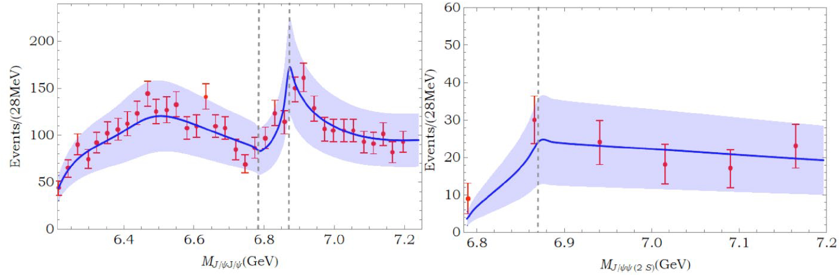
Parameter $ \chi^2/d.o.f $ 

$ g' $ 

$ N_1 $ 

$ N_2 $ 

$ \alpha_2 $ 

$ \alpha_3 $ 

Fit $ 0.93 $ 

$ -18.3\pm 1.6 $ 

$ 23\pm 10 $ 

$ 0.34\pm 0.23 $ 

$ -4.94\pm 0.02 $ 

$ 3.97\pm 0.05 $ 

$c_5$ 

$c_6$ 

$c_7$ 

$c_8$ 

$c_9$ 

$11.34\pm 0.05$ 

$50.79\pm0.05$ 

$-35.01\pm0.19$ 

$-64.71\pm 0.07$ 

$1.529\pm 0.002$ 

Table 1. Fit parameters of Fig. 4. The
$ c_i $ parameters are defined in Eq. (10). The errors are statistical only.During the fit, many solutions exist. Nevertheless, it was found that the triangle diagram contributions are all small. This behavior is unclear; however, one possible reason could be that the peak position through the anomalous threshold contribution, as shown in Fig. 3, is approximately 60 – 80 MeV above the
$ X(6900) $ peak; hence, the fit becomes difficult. One possible way to resolve the problem is to adopt another parameterization in which the background contributions are more flexible to be tuned. Thus, the interference between the background and the anomalous enhancement can lead to the shift of the peak position by a few tens of MeV. Another possible mechanism for the suppression of the triangle diagram is that the$ \psi(3770)D\bar D $ vertex is in the p-wave form; hence, it may provide another suppression factor due to (non-relativistic) power counting. [20]. We defer this investigation for future studies.
HTML
-
We would like to thank De-Liang Yao and Ling-Yun Dai for the very helpful discussions.


 DownLoad: