


 Abstract
 HTML
HTML Reference
 Related
 PDF
PDF


-
Spontaneous radioactivity of nuclei has always been an important and popular research field in nuclear physics and was first discovered by Becquerel in 1896 [1]. Soon after that, Rutherford observed the spontaneous emission of α particles from the nuclei in an experiment and named the process as α decay [2, 3]. It was not until 1928 that Gurdney and Condon as well as Gamow independently succeeded in providing a theoretical explanation of α decay using the tunneling effect of quantum mechanics [4–6]. Nowadays, many types of spontaneous radioactivity of nuclei are known to exist [7–12]. Cluster radioactivity is one such type that occurs mainly in the regions of heavy nuclei and is an intermediate process between α decay and spontaneous fission [13–16]. In this process, the parent nucleus emits a cluster particle that is heavier than an α particle but lighter than the lightest fission fragment while decaying into a doubly magic daughter nucleus 208Pb or its neighboring daughter nucleus [17–22]. This peculiar decay mode has aroused the interest of numerous physicists since it provides a considerable amount of vital information for studying the nuclear structure [23–27]. In 1980, Sǎndulescu, Poenaru, and Greiner made the first prediction of this radioactivity [28]. In 1984, Rose and Jones experimentally observed the emission of 14C from 223Ra, thus verifying this decay mode [29]. Currently, an increasing number of clusters ranging from 14C to 34Si have been observed experimentally to be emitted from the parent nuclei ranging from 221Fr to 242Cm, and their half-lives have been measured [30–33].
So far, there are numerous models and/or approaches proposed to fully comprehend cluster radioactivity, which are mainly divided into two extreme categories [34–50]. One is considered a spontaneous fission process with super asymmetric mass in an adiabatic state, in which the parent nucleus continuously deforms until it reaches the scission configuration after crossing the potential barrier [34–40]. The other is considered an α-like process in a non-adiabatic state, in which the cluster particle is preformed in the parent nucleus with a certain probability and then penetrates the potential barrier [41–52]. The former type of models, such as the Analytical Super Asymmetric Fission Model (ASAFM) of Poenaru et al. [34, 35], the Cubic-plus-Yukawa-plus-Exponential Potential Model (CYEM) of Shanmugam and Kamalaharan [36], the Coulomb and proximity potential model (CPPM) of Santhosh et al. [37], and so on [38–40], can accurately reproduce the experimenttal data of the cluster radioactivity half-lives. Among the latter type of models is the Preformed Cluster Model (PCM), where the cluster preformation probability is calculated by solving the Schr
$ \ddot{o} $ dinger equation for the dynamic flow of charges and masses by Gupta and Malik [41]. Ren et al. also provide a strong supporting proof for this type by considering the influence of charge number on the preformation factor under the framework of the microscopic densitydependent model (DDCM) with the renormalized M3Y nucleon-nucleon interaction to successfully calculate the cluster radioactivity half-lives [42] and so on [43–52]. At the same time, some valid empirical and/or semi-empirical formulae can be applied to calculate the half-life of cluster radioactivity, such as the universal decay law (UDL) proposed by Qi et al. [53, 54], the unified formula of half-lives for α decay and cluster radioactivity proposed by Ni et al. [55], the scaling law (SL) in cluster radioactivity proposed by Horoi et al. [56], and so on [57–63].In the 1970s, the proximity potential was first proposed by Blocki et al. to deal with heavy-ion reactions [64]. It is a nucleus-nucleus interaction potential based on the proximity force theorem, which is described as the product of two parts [65]. One is a factor determined by the mean curvature of the interaction surface, and the other is a universal function that depends on the separation distance and is independent of the masses of colliding nuclei [66]. The concept of the universal function is the fundamental advantage of proximity potential, since it has the merits of simple and precise formalism. Nowadays, the proximity potential has various versions with different characteristics from the original version (Prox.1977) [64] by improving the surface energy coefficients, the universal function, nuclear radius parameterization, and so on [67–86], which have been applied to different fields for comparative study by nuclear physicists [87–96]. It has also been extensively researched in the field of cluster radioactivity [41, 97, 98]. In 2012, Kumar et al. conducted research showing that the proximity potential 1977 could be a better option for studying cluster radioactivity by using 8 different versions of proximity potential formalisms and the preformation probability obtained by solving the stationary Schrödinger equation for the dynamic flow of mass and charge in a preformed cluster model (PCM) [41]. In 2016, Zhang et al. showed that the calculated results of Bass77 and Denisov potentials were most consistent with experimental data for large cluster radioactivity of even-even nuclei by comparing 14 different proximity potential formalisms [97]. Soon after, Santhosh et al. concluded that Bass80 was the most appropriate potential for studying cluster radioactivity by using a simple power-law interpolation to calculate the penetration probability inside the barrier as the preformation probability and comparing the calculations from 12 different versions of proximity potential formalisms [98]. The above researchers obtained different conclusions when determining the most suitable proximity potential formalism for the study of cluster radioactivity. This may be due to discrepancies in the evaluation of cluster preformation probability, the different types and numbers of proximity potential formalisms adopted, the inclusion of nuclear deformation, and so on when the cluster radioactivity half-lives are calculated. Therefore, it is necessary to explore the systematic behavior of more different proximity potentials and to select the most promising proximity potential formalism for cluster radioactivity. To this end, considering the preformation probability with a simple mass dependence on the emitted cluster, we systematically study the half-lives of cluster radioactivity for 26 trans-lead nuclei using CPPM with 28 different versions of proximity potential formalisms, which are all known proximity potential formalisms currently. The calculated results indicate that Prox.77-12 and Prox.81 are the best two with the lowest root-mean-square deviation for the study of cluster radioactivity.
The remainder of this article is organized as follows. The theoretical framework of CPPM with 28 different proximity potential formalisms and the compared semi-empirical and/or empirical formulae are exhaustively introduced in Sec. II. The results and discussion are distinctly presented in Sec. III. Finally, a brief summary is given in Sec. IV.
-
The cluster radioactivity half-life can be determined from [99]
$ {T}_{1/2} = \frac{\ln 2}{\lambda}=\frac{\ln 2}{\nu{S}_{c}{P}}, $

(1) where λ is the decay constant, and ν is the assault frequency on the barrier per second, which is taken as
$ 1.0\times10^{22} \rm s^{-1} $ in this work [100–102].$ {S}_{c} $ is the penetrability of barrier internal part (equal to the preformation probability of the cluster at the nuclear surface in a α-like theory). It has been suggested that, in the case of heavy cluster radioactivity [13],$ {S}_{c} $ can be expressed as$ {S}_{c}=({S}_{\alpha})^{({A_{c}-1})/{3}}, $

(2) where
$ A_{c} $ is the mass number of the cluster and$ {S}_{\alpha} $ is the preformation probability for the α decay. In different models, some investigators obtained similar$ {S}_{\alpha} $ values by fitting the experimental data [48, 49, 103, 104]. In this study, we choose$ {S}_{\alpha}=0.02897 $ for even-even parent nuclei and$ {S}_{\alpha}=0.0214 $ for odd-A parent nuclei [48]. The cluster radioactivity penetration probability through the potential barrier P can be calculated by using the semiclassical WKB approximation action integral and expressed as$ P=\exp\left(-\frac{2}{\hbar}\int_{R_{\rm in}}^{R_{\rm out}}\sqrt{{2\mu}\left\lvert{V(r)-Q_{c}}\right\rvert}{\rm d}r\right), $

(3) where
$ \hbar $ is the reduced Planck constant.$ \mu=\dfrac{m_{d}m_{c}}{m_{d}+m_{c}} $ is the reduced mass of emitted cluster-daughter nucleus system, with$ m_{d} $ and$ m_{c} $ being the daughter nucleus and the emitted cluster mass, respectively [97].$ Q_{c} $ represents the cluster radioactivity released energy. It can be obtained by using [105]$ Q_{c}=B(A_{c}, Z_{c})+B(A_{d}, Z_{d})-B(A_{p}, Z_{p}), $

(4) where
$ B(A_{c}, Z_{c}) $ ,$ B(A_{d}, Z_{d}) $ , and$ B(A_{p}, Z_{p}) $ are the binding energies of the emitted cluster, daughter nucleus, and parent nucleus, respectively. They are taken from AME2020 [106] and NUBASE2020 [107].$A_{c},~ Z_{c}$ ,$A_{d},~ Z_{d}$ , and$A_{p},~ Z_{p}$ are the mass and proton numbers of the emitted cluster, daughter nucleus, and parent nucleus, respectively.The total interaction potential
$ V(r) $ between the emitted cluster and daughter nucleus comprises the nuclear potential$ V_{N}(r) $ , Coulomb potential$ V_{C}(r) $ , and centrifugal potential$ V_{\ell}(r) $ . It can be expressed as$ V(r)=V_{N}(r)+V_{C}(r)+V_{\ell}(r). $

(5) In this study, we adopt the proximity potential formalism to substitute for the nuclear potential
$ V_{N}(r) $ . Detailed information on this is given in Sec. II.B. The Coulomb potential$ V_{C}(r) $ is taken as the potential of a uniformly charged sphere with radius R, which can be expressed as$ V_{C}(r)=\left\{\begin{array}{*{20}{l}} {\dfrac{Z_{c}Z_{d}e^{2}}{2R}\left[3-\left(\dfrac{r}{R}\right)^{2}\right], }&{r\leq R, }\\{\dfrac{Z_{c}Z_{d}e^{2}}{r}, }&{r>R, } \end{array}\right. $

(6) where
$ e^{2}=1.4399652 $ MeV$ \cdot $ fm is the square of the electronic elementary charge.$ R=R_{d}+R_{c} $ is the sharp radius, with$ R_{d} $ and$ R_{c} $ being the radii of the daughter nucleus and emitted cluster, respectively. Various expressions for$ R_{i} (i=c, d) $ within different proximity potential formalisms are in the Sec. II.B.For the centrifugal potential
$ V_{\ell}(r) $ , we adopt the Langer modified form since$ {\ell}({\ell+1})\to({\ell+\dfrac{1}{2}})^{2} $ is a necessary correction for one-dimensional problems [108]. It can be written as$ V_{\ell}(r)=\frac{\left(\ell+1/2\right)^{2}\hbar^{2}}{2\mu{r}^{2}}, $

(7) where
$ \ell $ is the angular momentum carried by the emitted cluster, which can be obtained via [12]$ \ell=\left\{\begin{array}{*{20}{l}} {\Delta_{j}, }& {{\rm{for\; even}} \; \Delta_{j} \;{\rm{and}}\; \pi_{p} = \pi_{d} , } \\ {\Delta_{j}+1, }&{{\rm{for\; even}} \; \Delta_{j} \;{\rm{and}}\; \pi_{p} \neq \pi_{d} , } \\ {\Delta_{j}, }& {{\rm{for\; odd}} \; \Delta_{j} \;{\rm{and}}\; \pi_{p} \neq \pi_{d} , }\\ {\Delta_{j}+1, } &{{\rm{for\; odd}} \;\Delta_{j} \;{\rm{and}}\; \pi_{p} = \pi_{d} .} \end{array}\right. $

(8) Here,
$ \Delta_{j} $ =$ \lvert {j_{p}-j_{d}-j_{c}} \rvert $ .$ j_{c} $ and$ \pi_{c} $ are the isospin and parity values of the emitted cluster,$ j_{d} $ and$ \pi_{d} $ are those of the daughter nucleus, and$ j_{p} $ and$ \pi_{p} $ are those of the parent nucleus, respectively. They are taken from NUBASE-2020 [107]. As for the bounds of the integral in Eq. (3),$ R_{\rm out}=\dfrac{Z_{c}Z_{d}e^{2}}{2Q_{c}}+ $ $\sqrt{\left(\dfrac{Z_{c}Z_{d}e^{2}}{2Q_{c}}\right)^{2}+\dfrac{\hbar^{2}(l+1/2)^{2}}{2\mu Q_{c}}}$ and$R_{\rm in}=R_{d}+ R_{c}$ are the radii for the separation configuration and the outer turning point, respectively [49]. -
In this study, we choose 28 versions of proximity potential formalisms to calculate the emitted cluster-daughter nucleus nuclear potential
$ V_{N}(r) $ , which are (i) Prox.77 [64] and its 12 modified forms to adjust the surface energy coefficient$ \gamma_{0} $ and$ k_{s} $ [67–75], (ii) Prox.81 [65], (iii) Prox.00 [76] and its revised versions Prox.00DP [66], Prox.2010 [77], and Dutt2011 [78], (iv) Bass73 [79] and its revised versions Bass77 [80] and Bass80 [81], (v) CW76 [82] and its revised versions BW91 [81] and AW95 [83], (vi) Ng$ \hat{o} $ 80 [84], (vii) Denisov [85] and its revised version Denisov DP [66], and (viii) Guo2013 [86]. Their detailed expressions are listed as follows. -
In the 1970s, the original version of the proximity potential formalism for two spherical interacting nuclei was proposed by Blocki et al. [64], which can be expressed as
$ V_{N}(r)=4\pi\gamma{b}\bar{R}\Phi(\xi). $

(9) Here, γ is the surface energy coefficient based on the Myers and Świa¸tecki formula [67]. It is written in the following form
$ \gamma=\gamma_{0}(1-k_{s}I^{2}), $

(10) where
$ I=\dfrac{N_{p}-Z_{p}}{A_{p}} $ is the asymmetry parameter and refers to the neutron-proton excess of the parent nucleus with$ N_{p} $ ,$ Z_{p} $ , and$ A_{p} $ being the neutron, proton, and mass numbers of the parent nucleus, respectively.$ \gamma_{0} $ and$ k_{s} $ are the surface energy constant and the surface asymmetry constant of Prox.77 and its modifications, respectively. Their details are listed in Table 1.γ set $ \gamma_{0} $ (MeV/fm2)

$ k_{s} $ 

References Set1(γ-MS 1967) 0.9517 1.7826 [67] Set2(γ-MS 1966) 1.01734 1.79 [68] Set3(γ-MN 1976) 1.460734 4.0 [69] Set4(γ-KNS 1979) 1.2402 3.0 [70] Set5(γ-MN-I 1981) 1.1756 2.2 [71] Set6(γ-MN-II 1981) 1.27326 2.5 [71] Set7(γ-MN-III 1981) 1.2502 2.4 [71] Set8(γ-RR 1984) 0.9517 2.6 [72] Set9(γ-MN 1988) 1.2496 2.3 [73] Set10(γ-MN 1995) 1.25284 2.345 [74] Set11(γ-PD-LDM 2003) 1.08948 1.9830 [75] Set12(γ-PD-NLD 2003) 0.9180 0.7546 [75] Set13(γ-PD-LSD 2003) 0.911445 2.2938 [75] Table 1. Different sets of surface energy coefficients.
$ \gamma_{0} $ and$ k_{s} $ are the surface energy constant and surface asymmetry constant, respectively.$ \bar{R} $ is the mean curvature radius or reduced radius. It can be obtained from$ \bar{R}=\frac{C_{c}C_{d}}{C_{c}+C_{d}}, $

(11) where
$ C_{i}=R_{i}\left[1-\left(\dfrac{b}{R_{i}}\right)^{2}\right] $ $(i= c, d)$ represents the matter radius of the emitted cluster$ (i=c) $ and daughter nucleus$ (i=d) $ , respectively.$ R_{i}=1.28A_{i}^{1/3}-0.76+0.8A_{i}^{-1/3} $ $(i= c, d)$ is the effective sharp radius, with$ A_{i} $ being the mass number of the emitted cluster$ (i=c) $ and daughter nucleus$ (i=d) $ , respectively. The diffuseness of nuclear surface b is considered close to unity ($ b\approx 1 $ fm). The universal function$ \Phi(\xi) $ is expressed as$ \Phi(\xi)=\left\{\begin{array}{*{20}{l}} {-\dfrac{1}{2}(\xi-2.54)^{2}-0.0852(\xi-2.54)^{3}, }&{\xi<1.2511, }\\ {-3.437\exp\Big(-\dfrac{\xi}{0.75}\Big), }&{\xi\geq{1.2511}, }\end{array}\right. $

(12) where
$ \xi=\dfrac{r-C_{c}-C_{d}}{b} $ is the distance between the near surface of the emitted cluster and daughter nucleus. -
In 1981, a new proximity potential formalism was proposed by Blocki and Swiątecki based on the proximity force theorem, which is labeled as Prox.81 [65]. It has the same form as Prox.77 [64], except for the surface energy coefficient
$ \gamma=0.9517 \left[1-1.7826 \left(\dfrac{N_{p}-Z_{p}}{A_{p}}\right)^{2}\right] $ and the universal function$ \Phi \left(\xi=\dfrac{r-C_{c}-C_{d}}{b}\right) $ written as$ \Phi(\xi)=\left\{\begin{array}{l} {-1.7817+0.9270\xi+0.143\xi^{2}-0.09\xi^{3}, \quad\xi<0, }\\{-1.7817+0.9270\xi+0.01696\xi^{2}}\\{-0.05148\xi^{3}, \qquad\qquad\qquad\qquad 0\leq\xi\leq{1.9475}, }\\{-4.41\exp\left(-\dfrac{\xi}{0.7176}\right), \qquad\qquad\qquad\ \xi>{1.9475}.}\end{array}\right. $

(13) -
In 2000, Myers et al. proposed a fresh proximity potential formalism to study the cross sections of synthesis new superheavy nuclei [76]. It is labeled as Prox.00 and expressed as
$ V_{N}(r)=4\pi\gamma{b}\bar{R}\Phi(\xi), $

(14) where b is the width parameter taken as unity. γ is the surface energy coefficient given by
$ \gamma=\frac{1}{4\pi{r_{0}^{2}}}{\left[18.63-Q\frac{(t_{c}^{2}+t_{d}^{2})}{2r_{0}^{2}}\right]}, $

(15) with neutron skin of nucleus
$ t_{i}=\frac{3}{2}r_{0}\left[\frac{J\left(\dfrac{N_{i}-Z_{i}}{A_{i}}\right)-\dfrac{1}{12}gZ_{i}A_{i}^{-1/3}}{Q+\dfrac{9}{4}A_{i}^{-1/3}}\right], \qquad (i=c, d). $

(16) Here,
$ r_{0}=1.14 $ fm, the nuclear symmetric energy coefficient$ J=32.65 $ MeV,$ g=0.757895 $ MeV, and the neutron skin stiffness coefficient$ Q=35.4 $ MeV [76].$ N_{i} $ ,$ Z_{i} $ , and$ A_{i} $ $ (i=c, d) $ refer to the neutron, proton, and mass numbers of the emitted cluster and daughter nuclei, respectively.$ \bar{R}=\dfrac{C_{c}C_{d}}{C_{c}+C_{d}} $ is the mean curvature radius.$ C_{c} $ and$ C_{d} $ are the matter radii of the emitted cluster and daughter nucleus, which can expressed as$ C_{i}=c_{i}+\frac{N_{i}}{A_{i}}t_{i}, \qquad (i=c, d), $

(17) with the half-density radius of the charge distribution
$ c_{i}=R_{i}\left(1-\frac{7b^{2}}{R_{i}^{2}}-\frac{49b^{4}}{8R_{i}^{4}}\right), \qquad(i=c, d). $

(18) Here,
$ R_{i} $ is the nuclear charge radius, which can be expressed as$ R_{i}=1.256A_{i}^{1/3}\left[1-0.202\left(\frac{N_{i}-Z_{i}}{A_{i}}\right)\right], \qquad (i=c, d). $

(19) The universal function
$ \Phi(\xi=\dfrac{r-C_{c}-C_{d}}{b}) $ is expressed as$ \Phi(\xi)=\left\{\begin{array}{*{20}{l}} {-0.1353+\sum_{n=0}^{5}\dfrac{c_{n}}{n+1}(2.5-\xi)^{n+1}, }&{0<\xi<2.5, }\\{-0.9551\exp\left(\dfrac{2.75-\xi}{0.7176}\right), }&{\xi\geq{2.5}, } \end{array}\right. $

(20) where the values of different constants
$ c_{n} $ are$c_{0}= -0.1886$ ,$ c_{1}=-0.2628 $ ,$ c_{2}= -0.15216 $ ,$ c_{3}=-0.04562 $ ,$ c_{4}=-0.069136 $ , and$ c_{5}=-0.011454 $ [76]. -
A modified version of Prox.00 was proposed by Dutt et al. using a more precise radius formula given by Royer and Roisseau [109], which is labeled as Prox.00 DP [66]. It is the same as Prox.00 except for the nuclear charge radius
$ R_{i} $ written as$ \begin{aligned}[b] R_{i} =\;&1.2332A_{i}^{1/3}+\frac{2.8961}{A_{i}^{2/3}} - 0.18688A_{i}^{1/3}\frac{N_{i}-Z_{i}}{A_{i}}, ~~ (i=c, d). \end{aligned} $

(21) -
In 2010, Dutt and Bensal presented another modified version of Prox.00 denoted as Prox.2010 [77]. It has the same form as Prox.00 DP except for the surface energy coefficient
$\gamma=1.25284\left[1-2.345\left(\dfrac{N_{p}-Z_{p}}{A_{p}}\right)^{2}\right]$ and the universal function$\Phi\left(\xi=\dfrac{r-C_{c}-C_{d}}{b}\right)$ written as$ \Phi(\xi)=\left\{\begin{array}{l}{-1.7817+0.9270\xi+0.143\xi^{2}-0.09\xi^{3}, \quad\xi<0, }\\{-1.7817+0.9270\xi+0.01696\xi^{2}}\\{-0.05148\xi^{3}}, \qquad\qquad\qquad\qquad 0\leq\xi\leq{1.9475}, \\ -4.41\exp\left(-\dfrac{\xi}{0.7176}\right), \qquad\qquad\quad\ \xi>{1.9475}.\end{array}\right. $

(22) -
Based on Prox.77, Dutt presented a new version of the potential, which is labeled as Dutt2011 [78]. It has the same form as Prox.2010 except for the nuclear charge radius
$ R_{i} $ written as$ R_{i}=1.171A_{i}^{1/3}+1.427A_{i}^{-1/3}, \qquad(i=c, d). $

(23) -
In 1973, Bass obtained the nuclear potential with the difference in surface energies between finite and infinite separations based on the liquid drop model [79]. It is labeled as Bass73 and expressed as
$ V_{N}(r)=\frac{-da_{s}A_{c}^{1/3}A_{d}^{1/3}}{R}\exp\left(-\frac{r-R}{d}\right), $

(24) where
$ R=R_{c}+R_{d}=r_{0}(A_{c}^{1/3}+A_{d}^{1/3}) $ is the sum of the half-maximum density radii, where$ r_{0}=1.07 $ fm,$ R_{c} $ and$ A_{c} $ are the radius and mass number of the daughter nucleus, respectively, and$ R_{d} $ and$ A_{d} $ are the radius and mass number of the emitted cluster, respectively.$ a_{s}=17.0 $ MeV and$ d=1.35 $ fm are the surface term in the liquid drop model mass formula and the range parameter, respectively. -
For the Bass77, the nuclear potential
$ V_{N} $ is given by [80]$ V_{N}(r)=-\frac{R_{c}R_{d}}{R_{c}+R_{d}}\Phi(s), $

(25) where
$ R_{i}=1.16A_{i}^{1/3}-1.39A_{i}^{-1/3} $ $ (i=c, d) $ is the half-density radius, with$ A_{i} $ being the mass number of the emitted cluster$ (i=c) $ and daughter nucleus$ (i=d) $ . The universal function$ \Phi(s=r-R_{c}-R_{d}) $ can be given by$ \Phi(s)=\left[0.03\exp\left(\frac{s}{3.3}\right)+0.0061\exp\left(\frac{s}{0.65}\right)\right]^{-1}. $

(26) -
Based on the proximity potential Bass77, Bass proposed an improved proximity potential formalism, which is labeled as Bass80 [81]. It is expressed as
$ V_{N}(r)=-\frac{R_{c}R_{d}}{R_{c}+R_{d}}\Phi(s). $

(27) Here,
$ R_{i}=R_{si}(1-\dfrac{0.98}{R_{si}^{2}}) $ with$R_{si}=1.28A_{i}^{1/3}- 0.76+ 0.8A_{i}^{-1/3}$ $ (i=c, d) $ . The universal function$ \Phi(s=r-R_{c}- R_{d}) $ is written by$ \Phi(s)=\left[0.033\exp\left(\frac{s}{3.5}\right)+0.007\exp\left(\frac{s}{0.65}\right)\right]^{-1}. $

(28) -
In 1976, an empirical nuclear potential was proposed by Christensen and Winter based on the analysis of heavy-ion elastic scattering data [82]. It is labeled as CW76 and expressed as
$ V_{N}(r)=-50\frac{R_{c}R_{d}}{R_{c}+R_{d}}\Phi(s), $

(29) where
$ R_{c} $ and$ R_{d} $ are given by$ R_{i}=1.233A_{i}^{1/3}-0.978A_{i}^{-1/3}, \qquad(i=c, d). $

(30) The universal function
$ \Phi(s=r-R_{c}-R_{d}) $ has the following form$ \Phi(s)=\exp\left(-\frac{s}{0.63}\right). $

(31) -
In 1991, Broglia and Winther presented a more refined nuclear potential by taking the Woods-Saxon parameterization of the proximity potential CW76. It is labeled as BW91 and expressed as [81]
$ V_{N}(r)=-\frac{V_{0}}{1+\exp\left(\dfrac{r-R}{0.63}\right)} =-\frac{16\pi\gamma{a}\dfrac{R_{c}R_{d}}{R_{c}+R_{d}}}{1+\exp\left(\dfrac{r-R}{0.63}\right)}. $

(32) Here,
$ \gamma=0.95 \left[1-1.8 \left(\dfrac{N_{d}-Z_{d}}{A_{d}}\right)\left(\dfrac{N_{c}-Z_{c}}{A_{c}}\right)\right] $ is the surface energy coefficient, with$ N_{d} $ ,$ Z_{d} $ , and$ A_{d} $ being the neutron, proton, and mass numbers of the daughter nucleus and$ N_{c} $ ,$ Z_{c} $ , and$ A_{c} $ being those of the emitted cluster, respectively.$ a=0.63 $ fm and$ R=R_{c}+R_{d}+0.29 $ with$ R_{i}=1.233A_{i}^{1/3}-0.98A_{i}^{-1/3} (i=c, d) $ . -
For the Aage Withner (AW95) potential [83], the proximity potential expression and other parameters are the same as BW91, except for
$ a=\frac{1}{1.17(1+0.53(A_{c}^{-1/3}+A_{d}^{-1/3}))}, $

(33) and
$ R=R_{c}+R_{d} $ with$ R_{i}=1.2A_{i}^{1/3}-0.09 $ $ (i=c, d) $ . -
In 1980, H. Ng
$ \hat{o} $ and Ch. Ng$ \hat{o} $ obtained the nuclear potential part of the interaction potential between two heavy ions using the energy density formalism and Fermi distributions for the nuclear densities [84]. It is labeled as Ng$ \hat{o} $ and expressed as$ V_{N}(r)=\frac{C_{c}C_{d}}{C_{c}+C_{d}}\phi(\xi), $

(34) where
$ C_{i}=R_{i}\left[1-\left(\dfrac{b}{R_{i}}\right)^{2}\right] $ $ (i=c, d) $ represents the S$ \ddot{u} $ smann central radii of the emitted cluster and daughter nucleus. b is the diffuseness of nuclear surface taken as unity.$ R_{i} $ represents the sharp radii and is expressed as$ R_{i}=\frac{N_{i}R_{ni}+Z_{i}R_{pi}}{A_{i}}, \qquad(i=c, d), $

(35) where
$ R_{ji}=r_{0ji}A_{i}^{1/3} $ $ (j=p, n $ ,$ i=c, d) $ , with$ r_{0pi}=1.128 $ fm and$ r_{0ni}=1.1375+1.875\times10^{-4}A_{i} $ fm. The universal function$ \phi(\xi=r-C_{c}-C_{d}) $ is given by$ \Phi(\xi)=\left\{\begin{array}{*{20}{l}} {-33+5.4(\xi+1.6)^{2}, }&{\xi<-1.6, }\\{-33\exp(-\dfrac{1}{5}(s+1.6)^{2}), }&{\xi\geq{-1.6}.}\end{array}\right. $

(36) -
By choosing 119 spherical or near spherical even-even nuclei around the β-stability line, Denisov presented a simple analytical expression for the nuclear potential of ion-ion interaction potential using the semi-microscopic approximation between all possible nucleus-nucleus combinations [85]. It is labeled as Denisov and expressed as
$\begin{aligned}[b] V_{N}(r)=\; & -1.989843\frac{R_{c}R_{d}}{R_{c}+R_{d}}\Phi(s)\times[1+0.003525139\\ & \times\left(\frac{A_{c}}{A_{d}}+\frac{A_{d}}{A_{c}}\right)^{3/2}-0.4113263(I_{c}+I_{d})], \end{aligned} $

(37) where
$ I_{i}=\dfrac{N_{i}-Z_{i}}{A_{i}} $ $ (i=c, d) $ is the isospin asymmetry.$ R_{i} $ is the effective nuclear radius and can be obtained by$ \begin{aligned}[b] R_{i} =\;&R_{0i}\left(1-\frac{3.413817}{R_{0i}}^{2}\right)\\ &+{1.284589\left(I_{i}-\frac{0.4A_{i}}{A_{i}+200}\right)}, \qquad (i=c, d), \end{aligned} $

(38) with
$ R_{0i}=1.240A_{i}^{1/3}\left(1+\frac{1.646}{A_{i}}-0.191I_{i}\right), \qquad (i=c, d). $

(39) The universal function
$ \Phi(s=r-R_{c}-R_{d}-2.65) $ is expressed as$ \Phi(s)=\left\{\begin{array}{l} \Bigg\{1-s^{2}\Bigg[0.05410106\dfrac{R_{c}R_{d}}{R_{c}+R_{d}}\exp\left(-\dfrac{s}{1.760580}\right) -0.5395420(I_{c}+I_{d})\exp\left(-\dfrac{s}{2.424408}\right)\Bigg]\Bigg\} \\ \quad \times\exp\left(-\dfrac{s}{0.7881663}\right), \qquad\qquad\quad\qquad\qquad{s\geq{0}}, \\ 1-\dfrac{s}{0.7881663}+1.229218s^{2}-0.2234277s^{3} -0.1038769s^{4}-\dfrac{R_{c}R_{d}}{R_{c}+R_{d}}(0.1844935s^{2}\\ \quad+0.07570101s^{3})+(I_{c}+I_{d}) (0.04470645s^{2}+0.03346870s^{3}),\quad\quad\quad\quad -5.65\leq{s}\leq{0}. \end{array}\right. $ 
(40) -
The proximity potential Denisov DP [66] is the modified version of Denisov using a more precise radius formula proposed by Royer et al. [109]. It is expressed as
$\begin{aligned}[b] R_{i} =\;&1.2332A_{i}^{1/3}+\frac{2.8961}{A_{i}^{2/3}} -0.18688A_{i}^{1/3}\frac{N_{i}-Z_{i}}{A_{i}}, ~~ (i=c, d). \end{aligned} $

(41) -
In 2013, Guo et al. presented a universal function of nuclear proximity potential from density-dependent nucleon-nucleon interaction using the double folding model [86]. It is labeled as Guo2013 and expressed as
$ V_{N}(r)=4\pi\gamma{b}\frac{R_{c}R_{d}}{R_{c}+R_{d}}\Phi(s), $

(42) where
$ \gamma=0.9517\left[1-1.7826\left(\dfrac{N_{p}-Z_{p}}{A_{p}}\right)^{2}\right] $ is the surface cofficient and$ R_{i}=1.28A_{i}^{1/3}-0.76+0.8A_{i}^{-1/3} $ $ (i=c, d) $ is the effective sharp radius. The universal function$\Phi\left(s=\dfrac{r-R_{c}-R_{d}}{b}\right)$ is expressed as$ \Phi(s)=\frac{p_{1}}{1+\exp\left(\dfrac{s+p_{2}}{p_{3}}\right)}, $

(43) where
$ p_{1}=-17.72 $ ,$ p_{2}=1.30 $ , and$ p_{3}=0.854 $ are the adjustable parameters. -
In 2009, a linear expression for charged-particle emissions was proposed by Qi et al. based on the α-like R-matrix theory and named as UDL [53, 54]. It can be expressed as
$ \log_{10}T_{1/2}=aZ_{c}Z_{d}\sqrt{\frac{{\cal{U}}}{Q_{c}}}+b\sqrt{{\cal{U}}Z_{c}Z_{d}(A_{c}^{1/3}+A_{d}^{1/3})}+c, $

(44) where
$ Q_{c} $ represents the cluster radioactivity released energy.$ {\cal{U}}=A_{c}A_{d}/(A_{c}+A_{d}) $ is the reduced mass of the emitted cluster-daughter nucleus system measured in units of the nucleon mass, with$ Z_{d} $ and$ A_{d} $ being the proton and mass numbers of the daughter nucleus and$ Z_{c} $ and$ A_{c} $ being those of the emitted cluster, respectively.$ a=0.4314 $ ,$ b=-0.3921 $ , and$ c=-32.7044 $ are the adjustable parameters [53, 54]. -
In 2008, Ni et al. proposed a unified formula of half-lives for α decay and cluster radioactivity by deducing from the WKB barrier penetration probability with some approximations [55]. It can be expressed as
$ \log_{10}T_{1/2}=a \sqrt{{\cal{U}}}Z_{c}Z_{d}Q_{c}^{-1/2}+b\sqrt{{\cal{U}}}(Z_{c}Z_{d})^{1/2}+c, $

(45) where
$ Q_{c} $ represents the α decay energy and cluster radioactivity released energy.$ {\cal{U}}=A_{c}A_{d}/(A_{c}+A_{d}) $ is the reduced mass, the same as that for UDL. For cluster radioactivity, the adjustable parameters are$ a=0.38617 $ ,$ b=-1.08676 $ , and$ c=-21.37195 $ for even-even nuclei and$ c=-20.11223 $ for odd-A nuclei [55]. For α decay, the adjustable parameters are$ a=0.39961 $ ,$ b=-1.31008 $ , and$ c=-17.00698 $ for even-even nuclei;$ c=-16.26029 $ for even-odd nuclei; and$ c=-16.40484 $ for odd-even nuclei [55]. -
In 2004, Horoi et al. proposed the first model-independent scaling law to describe the regularities of the experimental data for cluster radioactivity [56], which can be expressed as
$ \log_{10}T_{1/2}=(a{\cal{U}}^{x}+b)\left[\frac{({Z_{c}Z_{d}})^{y}}{Q_{c}^{1/2}}-7\right]+(c{\cal{U}}^{x}+d), $

(46) where
$ Q_{c} $ and$ {\cal{U}}=\dfrac{A_{d}A_{c}}{A_{d}+A_{c}} $ are the same as those for UDL.$ a=9.1 $ ,$ b=-10.2, $ ,$ c=7.39 $ ,$ d=-23.2 $ ,$ x=0.416 $ , and$ y=0.613 $ are the adjustable parameters [56]. -
The main purpose of this research is to perform a comparative study of various proximity potential formalisms when applied to cluster radioactivity. In order to explore the most suitable proximity potential formalism for the cluster radioactivity, we systematically calculate the cluster radioactivity half-lives of 26 nuclei in the emission of clusters 14C, 20O, 23F, 24, 25, 26Ne, 28, 30Mg, and 32, 34Si from various parent nuclei 221Fr to 242Cm by using CPPM with 28 different versions of proximity potential formalisms. In addition, the universal decay law (UDL), Ni's empirical formula, and the scaling law (SL) are used. The calculated results and experimental data are detailedly listed in Table 2. In this table, the first to third columns are the cluster decay process, the cluster radioactivity released energy
$ Q_{c} $ , and the angular momentum$ \ell $ taken away by the emitted cluster, respectively. The last nine columns represent the experimental data of the cluster radioactivity half-lives and the calculated ones obtained using CPPM with 28 different versions of proximity potential formalisms, the UDL, Ni's empirical formula, and the SL in a logarithmic form, respectively. From this table, we can find that the results calculated by using Prox.77 and its 12 modified forms as well as Prox.81 and Ng$ \hat{o} $ 80 are within an order of magnitude from the experimental data on the whole, which indicates that the experimental data can faultlessly be reproduced. For Prox.00 and its revised versions Prox.00 DP, Prox.2010, and Dutt2011, as well as Guo2013, the calculations differ overall from the experimental data by two to four orders of magnitude. However, for Bass73 and its revised versions Bass77 and Bass80, as well as CW76 and its revised versions BW91 and AW95, the calculated values of the improved version are closer to the experimental data than those of the previous version. Denisov's calculated results are about one to three orders of magnitude more than the experimental data. However, the calculated results of its revised version, Denisov DP, are about six to eleven orders of magnitude less than the experimental data and about seven to thirteen orders of magnitude less than the Denisov results. The reduced order magnitude increases with the size of the cluster particle.Cluster decay $ Q_{c} $ / MeV

$ \ell $ 

$\log_{10}{T}_{1/2}/{\rm s}$ 

EXP Prox.77-1 Prox.77-2 Prox.77-3 Prox.77-4 Prox.77-5 Prox.77-6 Prox.77-7 Prox.77-8 221Fr→207Tl+14C 31.29 3 14.56 14.82 14.71 14.17 14.43 14.46 14.31 14.35 14.89 221Ra→207Pb+14C 32.40 3 13.39 13.69 13.58 12.99 13.28 13.32 13.17 13.20 13.76 222Ra→208Pb+14C 33.05 0 11.22 11.80 11.68 11.09 11.39 11.42 11.26 11.30 11.86 223Ra→209Pb+14C 31.83 4 15.05 14.72 14.61 14.06 14.33 14.36 14.21 14.24 14.79 224Ra→210Pb+14C 30.53 0 15.87 16.39 16.27 15.75 16.01 16.03 15.89 15.92 16.45 226Ra→212Pb+14C 28.20 0 21.20 21.28 21.17 20.70 20.93 20.95 20.81 20.84 21.34 223Ac→209Bi+14C 33.06 2 12.60 13.23 13.12 12.52 12.82 12.86 12.70 12.73 13.29 225Ac→211Bi+14C 30.48 4 17.16 18.18 18.07 17.54 17.80 17.83 17.69 17.72 18.24 228Th→208Pb+20O 44.72 0 20.73 21.73 21.59 20.89 21.23 21.27 21.08 21.12 21.82 231Pa→208Pb+23F 51.88 1 26.02 25.20 25.04 24.28 24.66 24.69 24.49 24.53 25.29 230Th→206Hg+24Ne 57.76 0 24.63 24.52 24.36 23.63 23.99 24.02 23.82 23.86 24.61 231Pa→207Tl+24Ne 60.41 1 22.89 22.91 22.74 21.96 22.35 22.39 22.18 22.22 23.00 232U→208Pb+24Ne 62.31 0 20.39 20.45 20.28 19.45 19.86 19.91 19.69 19.74 20.54 233U→209Pb+24Ne 60.49 2 24.84 23.95 23.79 23.01 23.40 23.44 23.23 23.27 24.04 234U→210Pb+24Ne 58.83 0 25.93 25.26 25.11 24.37 24.73 24.77 24.57 24.61 25.36 235U→211Pb+24Ne 57.36 1 27.42 28.46 28.31 27.61 27.95 27.98 27.78 27.83 28.55 233U→208Pb+25Ne 60.70 2 24.84 24.51 24.34 23.52 23.93 23.97 23.75 23.80 24.61 234U→208Pb+26Ne 59.41 0 25.93 26.10 25.93 25.11 25.51 25.55 25.33 25.38 26.20 234U→206Hg+28Mg 74.11 0 25.53 24.90 24.72 23.90 24.30 24.34 24.12 24.16 25.01 236U→208Hg+28Mg 70.73 0 27.58 29.28 29.11 28.36 28.72 28.75 28.54 28.59 29.38 236Pu→208Pb+28Mg 79.67 0 21.52 20.70 20.51 19.57 20.04 20.10 19.85 19.90 20.80 238Pu→210Pb+28Mg 75.91 0 25.70 25.10 24.92 24.08 24.50 24.54 24.31 24.36 25.20 236U→206Hg+30Mg 72.27 0 27.58 28.72 28.53 27.70 28.11 28.14 27.90 27.95 28.83 238Pu→208Pb+30Mg 76.79 0 25.70 25.45 25.26 24.33 24.79 24.84 24.58 24.64 25.56 238Pu→206Hg+32Si 91.19 0 25.28 25.02 24.82 23.87 24.34 24.39 24.13 24.19 25.13 242Cm→208Pb+34Si 96.54 0 23.15 23.01 22.79 21.69 22.24 22.30 22.01 22.07 23.14 Cluster decay $ Q_{c} $ / MeV

$ \ell $ 

$\log_{10}{T}_{1/2}/{\rm s}$ 

EXP Prox.77-9 Prox.77-10 Prox.77-11 Prox.77-12 Prox.77-13 Prox.81 Prox.00 Prox.00 DP 221Fr→207Tl+14C 31.29 3 14.56 14.33 14.33 14.60 14.80 14.93 14.75 14.26 11.87 221Ra→207Pb+14C 32.40 3 13.39 13.19 13.19 13.46 13.68 13.80 13.62 13.09 10.72 222Ra→208Pb+14C 33.05 0 11.22 11.28 11.28 11.56 11.78 11.91 11.73 11.27 8.91 223Ra→209Pb+14C 31.83 4 15.05 14.23 14.23 14.50 14.70 14.83 14.65 14.14 11.74 224Ra→210Pb+14C 30.53 0 15.87 15.91 15.91 16.17 16.36 16.49 16.32 15.78 13.36 226Ra→212Pb+14C 28.20 0 21.20 20.83 20.83 21.07 21.25 21.38 21.21 20.62 18.14 223Ac→209Bi+14C 33.06 2 12.60 12.72 12.72 13.00 13.22 13.34 13.16 12.63 10.27 225Ac→211Bi+14C 30.48 4 17.16 17.71 17.71 17.96 18.16 18.28 18.11 17.50 15.06 228Th→208Pb+20O 44.72 0 20.73 21.11 21.11 21.44 21.71 21.87 21.65 20.78 18.34 231Pa→208Pb+23F 51.88 1 26.02 24.52 24.52 24.88 25.17 25.35 25.11 24.05 21.62 Continued on next page Table 2. Comparison of the discrepancy between the experimental cluster radioactivity half-lives (in seconds) and calculated ones using CPPM with 28 different versions of the proximity potential formalisms, the UDL, Ni's empirical formula, and the SL in a logarithmic form. The experimental cluster radioactivity half-lives are taken from Ref. [59].
Table 2-continued from previous page Cluster decay $ Q_{c} $ / MeV

$ \ell $ 

$\log_{10}{T}_{1/2}/{\rm s}$ 

EXP Prox.77-9 Prox.77-10 Prox.77-11 Prox.77-12 Prox.77-13 Prox.81 Prox.00 Prox.00 DP 230Th→206Hg+24Ne 57.76 0 24.63 23.84 23.84 24.20 24.48 24.67 24.43 23.07 20.61 231Pa→207Tl+24Ne 60.41 1 22.89 22.21 22.20 22.58 22.88 23.06 22.82 21.49 19.07 232U→208Pb+24Ne 62.31 0 20.39 19.72 19.72 20.11 20.42 20.60 20.35 19.02 16.63 233U→209Pb+24Ne 60.49 2 24.84 23.26 23.26 23.63 23.92 24.10 23.86 22.47 20.04 234U→210Pb+24Ne 58.83 0 25.93 24.59 24.59 24.95 25.23 25.42 25.18 23.74 21.28 235U→211Pb+24Ne 57.36 1 27.42 27.81 27.81 28.16 28.43 28.61 28.37 26.91 24.42 233U→208Pb+25Ne 60.70 2 24.84 23.78 23.78 24.18 24.48 24.68 24.42 23.12 20.72 234U→208Pb+26Ne 59.41 0 25.93 25.36 25.36 25.76 26.07 26.27 26.01 24.77 22.36 234U→206Hg+28Mg 74.11 0 25.53 24.15 24.15 24.55 24.87 25.07 24.81 22.94 20.53 236U→208Hg+28Mg 70.73 0 27.58 28.57 28.57 28.95 29.23 29.44 29.18 27.24 24.77 236Pu→208Pb+28Mg 79.67 0 21.52 19.88 19.88 20.32 20.68 20.87 20.60 18.77 16.44 238Pu→210Pb+28Mg 75.91 0 25.70 24.35 24.34 24.75 25.07 25.27 25.00 23.07 20.67 236U→206Hg+30Mg 72.27 0 27.58 27.93 27.93 28.35 28.67 28.90 28.62 26.88 24.49 238Pu→208Pb+30Mg 76.79 0 25.70 24.62 24.62 25.07 25.42 25.63 25.35 23.59 21.26 238Pu→206Hg+32Si 91.19 0 25.28 24.17 24.17 24.62 24.98 25.20 24.91 22.56 20.22 242Cm→208Pb+34Si 96.54 0 23.15 22.05 22.05 22.57 22.98 23.22 22.90 20.74 18.52 Cluster decay $ Q_{c} $ / MeV

$ \ell $ 

$\log_{10}{T}_{1/2}/{\rm s}$ 

EXP Prox.2010 Dutt2011 Bass73 Bass77 Bass80 CW76 BW91 AW95 221Fr→207Tl+14C 31.29 3 14.56 12.23 12.07 16.22 15.77 14.86 13.38 13.68 13.64 221Ra→207Pb+14C 32.40 3 13.39 11.09 10.97 15.08 14.63 13.72 12.28 12.55 12.51 222Ra→208Pb+14C 33.05 0 11.22 9.28 9.15 13.12 12.61 11.72 10.45 10.63 10.62 223Ra→209Pb+14C 31.83 4 15.05 12.11 11.96 16.16 15.71 14.78 13.26 13.58 13.54 224Ra→210Pb+14C 30.53 0 15.87 13.72 13.55 17.89 17.46 16.51 14.86 15.26 15.20 226Ra→212Pb+14C 28.20 0 21.20 18.48 18.28 22.93 22.55 21.56 19.60 20.17 20.08 223Ac→209Bi+14C 33.06 2 12.60 10.63 10.53 14.64 14.17 13.25 11.83 12.09 12.06 225Ac→211Bi+14C 30.48 4 17.16 15.41 15.27 19.78 19.39 18.41 16.59 17.07 17.00 228Th→208Pb+20O 44.72 0 20.73 18.96 18.48 24.14 22.87 21.87 19.44 20.12 20.34 231Pa→208Pb+23F 51.88 1 26.02 22.40 21.77 28.07 26.41 25.34 22.54 23.35 23.72 230Th→206Hg+24Ne 57.76 0 24.63 21.47 20.89 27.62 25.91 24.79 21.60 22.53 22.92 231Pa→207Tl+24Ne 60.41 1 22.89 19.95 19.41 25.94 24.19 23.08 20.11 20.91 21.34 232U→208Pb+24Ne 62.31 0 20.39 17.52 17.03 23.45 21.67 20.58 17.71 18.44 18.89 233U→209Pb+24Ne 60.49 2 24.84 20.91 20.39 27.09 25.35 24.21 21.07 21.96 22.38 234U→210Pb+24Ne 58.83 0 25.93 22.14 21.58 28.51 26.79 25.62 22.26 23.27 23.68 235U→211Pb+24Ne 57.36 1 27.42 25.26 24.68 31.80 30.10 28.90 25.36 26.47 26.86 233U→208Pb+25Ne 60.70 2 24.84 21.63 21.01 27.68 25.77 24.66 21.63 22.48 22.95 234U→208Pb+26Ne 59.41 0 25.93 23.30 22.54 29.41 27.35 26.23 23.11 24.04 24.54 234U→206Hg+28Mg 74.11 0 25.53 21.67 21.08 28.65 26.45 25.22 21.50 22.55 23.16 236U→208Hg+28Mg 70.73 0 27.58 25.87 25.21 33.25 31.09 29.78 25.63 26.93 27.50 236Pu→208Pb+28Mg 79.67 0 21.52 17.63 17.15 24.31 22.04 20.83 17.54 18.34 19.00 238Pu→210Pb+28Mg 75.91 0 25.70 21.81 21.26 28.98 26.76 25.47 21.64 22.75 23.37 Continued on next page Table 2-continued from previous page Cluster decay $ Q_{c} $ / MeV

$ \ell $ 

$\log_{10}{T}_{1/2}/{\rm s}$ 

EXP Prox.2010 Dutt2011 Bass73 Bass77 Bass80 CW76 BW91 AW95 236U→206Hg+30Mg 72.27 0 27.58 25.69 24.84 32.69 30.21 28.95 25.14 26.31 26.98 238Pu→208Pb+30Mg 76.79 0 25.70 22.50 21.76 29.37 26.83 25.58 22.04 23.04 23.75 238Pu→206Hg+32Si 91.19 0 25.28 21.67 21.11 29.34 26.65 25.30 21.23 22.33 23.15 242Cm→208Pb+34Si 96.54 0 23.15 20.14 19.45 27.36 24.26 22.93 19.45 20.26 21.23 Cluster decay $ Q_{c} $ / MeV

$ \ell $ 

$\log_{10}{T}_{1/2}/{\rm s}$ 

EXP Ng $ \hat{o} $ 80

Denisov Denisov DP Guo2013 UDL Ni SL 221Fr→207Tl+14C 31.29 3 14.56 15.06 15.19 8.11 12.47 12.70 14.63 13.54 221Ra→207Pb+14C 32.40 3 13.39 13.95 14.01 7.01 11.36 11.46 13.48 12.27 222Ra→208Pb+14C 33.05 0 11.22 12.05 12.01 5.30 9.52 10.07 11.02 11.00 223Ra→209Pb+14C 31.83 4 15.05 14.97 15.10 7.97 12.35 12.57 14.56 13.42 224Ra→210Pb+14C 30.53 0 15.87 16.62 16.85 9.49 13.97 15.38 15.86 16.14 226Ra→212Pb+14C 28.20 0 21.20 21.50 21.94 14.06 18.77 20.95 20.94 21.53 223Ac→209Bi+14C 33.06 2 12.60 13.50 13.53 6.58 10.90 11.08 13.19 11.93 225Ac→211Bi+14C 30.48 4 17.16 18.43 18.75 11.09 15.71 16.61 18.24 17.26 228Th→208Pb+20O 44.72 0 20.73 22.09 22.98 13.36 18.73 21.97 21.54 21.20 231Pa→208Pb+23F 51.88 1 26.02 25.62 26.75 16.31 21.92 24.90 25.59 23.78 230Th→206Hg+24Ne 57.76 0 24.63 24.95 26.40 15.17 21.07 25.39 24.58 23.92 231Pa→207Tl+24Ne 60.41 1 22.89 23.36 24.69 13.64 19.51 22.27 23.09 21.32 232U→208Pb+24Ne 62.31 0 20.39 20.92 22.17 11.21 17.07 20.59 20.36 19.94 233U→209Pb+24Ne 60.49 2 24.84 24.41 25.80 14.57 20.51 23.63 24.41 22.55 234U→210Pb+24Ne 58.83 0 25.93 25.71 27.22 15.80 21.78 26.52 25.81 25.03 235U→211Pb+24Ne 57.36 1 27.42 28.90 30.51 18.96 24.95 29.16 29.51 27.31 233U→208Pb+25Ne 60.70 2 24.84 25.00 26.29 15.22 21.06 24.00 24.88 23.05 234U→208Pb+26Ne 59.41 0 25.93 26.60 27.91 16.83 22.58 27.01 26.52 25.84 234U→206Hg+28Mg 74.11 0 25.53 25.45 27.22 14.76 21.10 25.77 25.25 24.76 236U→208Hg+28Mg 70.73 0 27.58 29.80 31.80 19.14 25.43 31.25 30.33 29.28 236Pu→208Pb+28Mg 79.67 0 21.52 21.30 22.83 10.65 16.96 20.64 20.76 20.83 238Pu→210Pb+28Mg 75.91 0 25.70 25.67 27.48 14.87 21.27 26.26 25.96 25.42 236U→206Hg+30Mg 72.27 0 27.58 29.30 31.04 18.79 24.82 29.94 29.47 28.69 238Pu→208Pb+30Mg 76.79 0 25.70 26.08 27.66 15.42 21.58 26.06 26.10 25.71 238Pu→206Hg+32Si 91.19 0 25.28 25.70 27.66 14.16 20.89 25.48 25.59 25.70 242Cm→208Pb+34Si 96.54 0 23.15 23.79 25.41 12.38 18.90 22.35 23.48 24.21 In order to explore the specific reasons for this situation, taking the example of
$ ^{242}{\rm{Cm}}\to^{208}{\rm{Pb}}+^{34}{\rm{Si}} $ , we plot the total interaction potential$ V(r) $ between the emitted cluster and daughter nucleus using CPPM with Denisov and Denisov DP in Fig. 1. In addition, the nuclear potential calculated by the double folding approach is used to deeply comprehend the difference between the proximity potential and other nuclear potentials, which considers the nuclear density distributions and the effective nucleon-nucleon interactions. It also has been shown to be successfully applied to α decay [110], proton emission [111], two-proton radioactivity [112], and cluster radioactivity [113] in the density-dependent cluster model. In this study, we choose the monopole component of a realistic double folding potential plus Coulomb core-cluster potential (DFC) as the interaction potential to describe the cluster radioactivity. Its related data are taken from Ref. [114] and also plotted in Fig. 1. From this figure, we can find that the total interaction potential$ V(r) $ at short distances changes dramatically, which shows that the nuclear potential plays a dominating role, whereas the choice of different nuclear potentials may lead to enormous differences. At long distances,$ V(r) $ remains essentially constant, which should mainly be the effect of the Coulomb potential. Generally, the trend of the potential energy curve remains consistent. At the same time, the separation configuration radius$ R_{\rm in} $ of the improved Denisov DP is slightly increased compared with the original Denisov, but the outer turning point$ R_{\rm out} $ remains unchanged. Therefore, the integral result becomes smaller, and the penetration probability P is greater in Eq. (3), which will result in a smaller cluster radioactivity half-life. This is consistent with the conclusions in the Ref. [97]. For larger cluster particles, a higher cluster radioactivity released energy$ Q_{c} $ gives rise to a smaller outer turning point$ R_{\rm out} $ , which will further reduce the cluster radioactivity half-life. Consequently, there is a huge deviation between the calculated results of Denisov and Denisov DP, which is further expanded in larger cluster particles.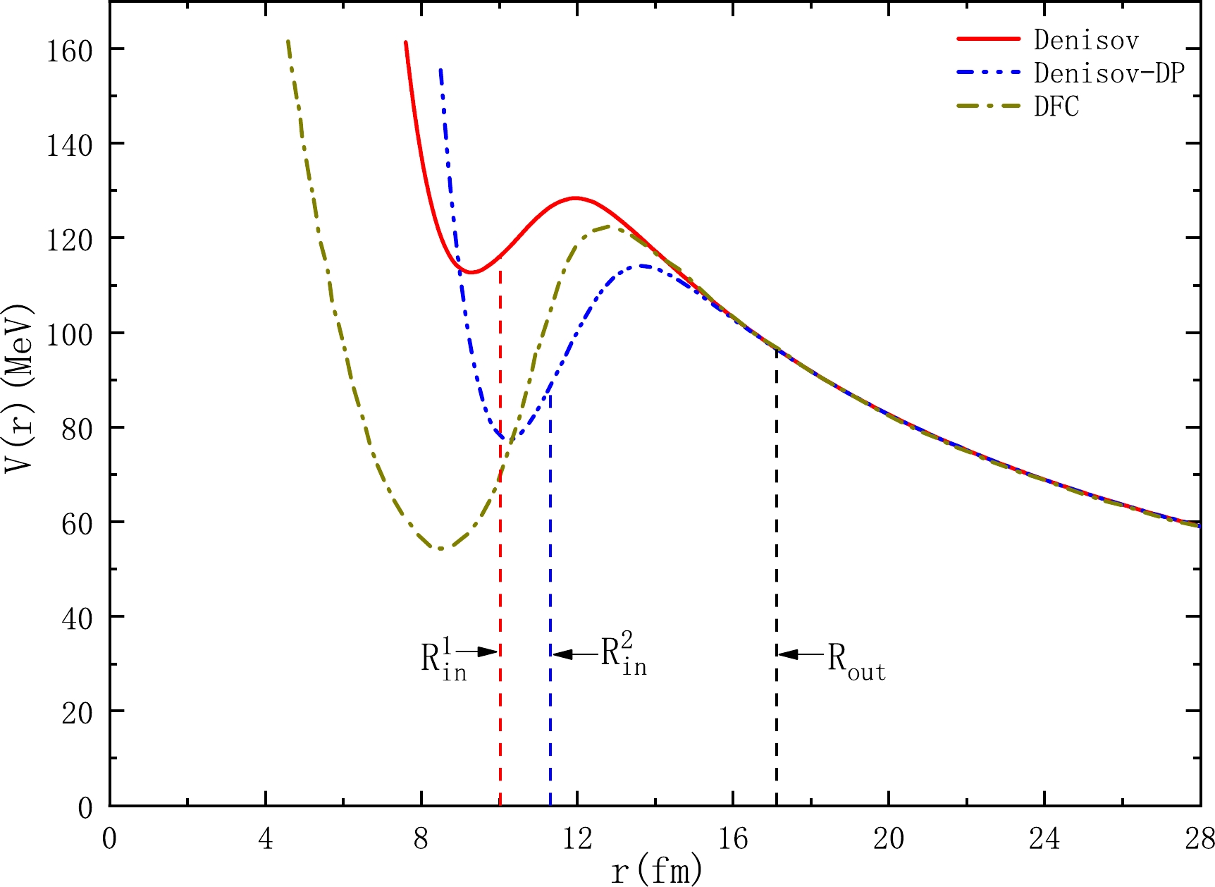
Figure 1. (color online) Schematic of the total interaction potential
$V(r)$ between the cluster and daughter nucleus obtained using CPPM with Denisov, Denisov DP, and DFC. The relevant data on DFC are obtained from Ref. [114].$R_{\rm in}^{1}$ and$R_{\rm in}^{2}$ are the radii for the separation configuration using Denisov and Denisov DP, respectively.$R_{\rm out}$ is the outer turning point.To intuitively survey the deviations between the calculated cluster radioactivity half-lives and experimental ones, we adopt the root-mean-square deviation σ as a measure in this work. It can be expressed as
$ \sigma = \sqrt{\sum\limits_{i=1}^{n}\frac{(\log_{10}{T_{1/2}^{{{\rm exp}, i}}}-\log_{10}{T_{1/2}^{{{\rm cal}, i}}})^2}{n}}, $

(47) where
$\log_{10}{T_{1/2}^{{{\rm exp}, i}}}$ and$\log_{10}{T_{1/2}^{{{\rm cal}, i}}}$ represent the logarithmic forms of the experimental cluster radioactivity half-lives and calculated ones for the i-th nucleus, respectively. n is the number of nuclei involved for different decay cases. The detailed calculations of root-mean-square deviation σ for 28 different versions of proximity potential formalisms are listed in Table 3. Additionally, the root-mean-square deviation σ obtained using the UDL, Ni's empirical formula, and the SL are presented in this table. From this table, the most suitable proximity potential formalisms for the cluster radioactivity can be obtained using Prox.77-12 and Prox.81 since both of them have the lowest root-mean-square deviation$ \sigma=0.681 $ . Simultaneously, some other proximity potential formalisms with a root-mean-square deviation σ less than 1 can also be applied to cluster radioactivity. Moreover, there are some proximity potential calculations with huge deviations from the experimental data, such as Denisov DP, Prox.00 DP, Guo2013, and Dutt2011. On the whole, the calculations by CPPM with different versions of proximity potential formalisms have comparable accuracies with respect to experimental data. To further verify the feasibility of applying the proximity potential to cluster radioactivity, we plot the differences between the experimental cluster radioactivity half-lives and the calculated ones using CPPM with Prox.77-12 and Prox.81, as well as the compared formulae in a logarithmic form, in Fig. 2. From this figure, we can clearly see that the deviations using CPPM with Prox.77-12 and Prox.81 are mainly within -1→1, whereas the deviation distributions of the UDL and SL are slightly dispersed. It demonstrates that Prox.77-12 and Prox.81 can be adopted to obtain the most precise calculations of cluster radioactivity half-lives among the 28 versions of proximity potential formalisms.Method Prox.77-1 Prox.77-2 Prox.77-3 Prox.77-4 Prox.77-5 Prox.77-6 Prox.77-7 Prox.77-8 σ 0.686 0.691 1.100 0.838 0.815 0.943 0.914 0.700 Method Prox.77-9 Prox.77-10 Prox.77-11 Prox.77-12 Prox.77-13 Prox.81 Prox.00 Prox.00 DP σ 0.924 0.924 0.730 0.681 0.715 0.681 1.594 3.771 Method Prox.2010 Dutt2011 Bass73 Bass77 Bass80 CW76 BW91 AW95 σ 2.915 3.391 3.146 1.566 0.763 2.779 2.006 1.594 Method Ng $ \hat{o} $ 80

Denisov Denisov DP Guo2013 UDL Ni SL σ 0.844 1.878 8.859 3.301 1.374 0.875 1.072 Table 3. Root-mean-square deviation σ between the experimental data and calculated ones using CPPM with 28 different versions of the proximity potential formalisms, the UDL, Ni's empirical formula, and the SL for cluster radioactivity.

Figure 2. (color online) Comparison of the discrepancy between the experimental cluster radioactivity half-lives and calculated ones using CPPM with Prox.77-12 and Prox.81 as well as the compared formulae in a logarithmic form.
Encouraged by the good agreement between the experimental cluster radioactivity half-lives and the calculated ones obtained using CPPM with Prox.77-12 and Prox.81, we employ four proximity potentials with the smallest root-mean-square deviation to predict the half-lives of 51 possible cluster radioactive candidates, whose cluster radioactivity is energetically allowed or observed but not yet quantified in NUBASE2020. Meanwhile, we also calculated their α decay half-lives and compared the results with the cluster radioactivity ones to determine the most dominant decay modes of these predicted nuclei. All the predicted results are listed in Table 4. In this table, the first to fourth columns are the parent nuclei, corresponding emitted particles, decay energies Q of α decay, cluster radioactivity, and orbital angular momentum
$ \ell $ carried by the emitted particles, respectively. The fifth column represents the experimental half-lives of α decay and the cluster radioactivity. The last five columns represent the predicted results obtained using CPPM with Prox.77-12, Prox.81, Prox.77-1, and Prox.77-2 and Ni's empirical formula in a logarithmic form, respectively. The decay energies and experimental half-lives of α decay are taken from AME2020 [106] and NUBASE2020 [107]. At the same time, we introduce the branching ratio of cluster radioactivity relative to that of α decay$\varsigma={\rm log}_{10}{T}_{1/2}^{\ \alpha}- {\rm log}_{10}{T}_{1/2}^{\ C}$ [115] to manifest the competition among the two. From this table, we can find that the range of ς from approximately –11 to –20 is significantly less than 0, which indicates that these predicted nuclei are more likely to undergo α decay than cluster radioactivity. In addition, the predicted results obtained using CPPM with four proximity potentials and Ni's empirical formula remained on approximately the same order of magnitude for cluster radioactivity and well reproduced the experimental data for α decay. We plot the the logarithmic half-lives of CPPM with minimum root-mean-square deviation proximity potentials and Ni's empirical formula in Fig. 3 to intuitively investigate the agreement of our predicted results with Ni's empirical formula in cluster radioactivity. From this figure, it is obvious that the calculated results obtained using CPPM with Prox.77-12 and Prox.81 are very close to those obtained with Ni's empirical formula, which indicates that CPPM with the proximity potential is reliable for calculating cluster radioactivity half-lives. We also hope that these predicted results will be useful for exploring new radioactive nuclei clusters in future experiments.Parent nuclei Emitted particles Q/MeV $ \ell $ 

$\log_{10}{T}_{1/2}/{\rm s}$ 

EXP Prox.77-12 Prox.81 Prox.77-1 Prox.77-2 Ni 219Rn 4He 6.95 2 0.60 0.21 0.18 0.22 0.18 0.55 14C 28.10 3 − 20.48 20.43 20.50 20.39 20.28 220Rn 4He 6.40 0 1.75 2.00 1.97 2.01 1.96 1.93 14C 28.54 0 − 18.76 18.71 18.78 18.67 18.05 221Fr 4He 6.46 2 2.46 2.55 2.52 2.56 2.51 2.71 15N 34.12 3 − 22.14 22.10 22.16 22.06 22.16 223Ra 4He 5.98 2 5.99 5.14 5.11 5.14 5.10 5.39 18O 40.30 1 − 26.19 26.14 26.21 26.09 26.42 225Ra 4He 5.10 4 − 10.43 10.40 10.44 10.40 10.01 14C 29.47 4 − 19.28 19.24 19.31 19.20 19.36 20O 40.48 1 − 28.12 28.07 28.15 28.01 28.35 226Ra 4He 4.87 0 10.70 10.96 10.93 10.97 10.93 10.67 20O 40.82 0 − 26.54 26.49 26.57 26.44 26.41 223Ac 4He 6.78 2 2.10 2.10 2.07 2.10 2.06 2.27 15N 39.47 3 >14.76 14.57 14.51 14.58 14.47 14.47 227Ac 4He 5.04 0 10.70 10.53 10.50 10.53 10.50 10.73 20O 43.09 1 − 24.30 24.25 24.33 24.19 24.54 229Ac 4He 4.44 1 − 14.76 14.74 14.77 14.73 14.75 23F 48.35 2 − 28.73 28.68 28.77 28.61 29.13 226Th 4He 6.45 0 3.27 3.51 3.48 3.52 3.48 3.44 18O 45.73 0 − 18.17 18.11 18.19 18.06 17.81 14C 30.55 0 >16.76 18.14 18.09 18.16 18.05 17.82 227Th 4He 6.15 2 6.21 5.21 5.18 5.22 5.18 5.51 18O 44.20 4 >15.36 21.48 21.43 21.50 21.37 21.69 228Th 4He 5.52 0 7.78 8.06 8.03 8.06 8.02 7.88 22Ne 55.74 0 − 25.86 25.80 25.88 25.74 26.07 229Th 4He 5.17 2 11.40 10.45 10.43 10.46 10.42 10.61 20O 43.40 2 − 24.84 24.79 24.87 24.73 25.26 24Ne 57.83 3 − 25.53 25.47 25.56 25.40 25.71 231Th 4He 4.21 2 − 17.35 17.33 17.36 17.32 17.24 24Ne 56.25 2 − 27.78 27.73 27.82 27.66 28.36 25Ne 56.80 2 − 27.85 27.80 27.89 27.73 28.30 232Th 4He 4.08 0 17.65 18.09 18.07 18.10 18.06 17.57 24Ne 54.67 0 >29.20 29.22 29.17 29.26 29.11 29.86 26Ne 55.91 0 >29.20 29.01 28.96 29.06 28.89 29.45 227Pa 4He 6.58 0 3.43 3.52 3.49 3.52 3.48 3.92 18O 45.87 2 − 19.77 19.70 19.78 19.65 20.01 229Pa 4He 5.84 1 7.43 7.04 7.01 7.04 7.00 7.30 22Ne 58.96 2 − 23.27 23.21 23.29 23.15 23.62 230U 4He 5.99 0 6.24 6.54 6.51 6.54 6.50 6.41 Continued on next page Table 4. Predicted half-lives for 51 possible cluster radioactive nuclei.
Table 4-continued from previous page Parent nuclei Emitted particles Q/MeV $ \ell $ 

$\log_{10}{T}_{1/2}/{\rm s}$ 

EXP Prox.77-12 Prox.81 Prox.77-1 Prox.77-2 Ni 22Ne 61.39 0 >18.20 20.14 20.07 20.15 20.00 20.09 24Ne 61.35 0 >18.20 21.88 21.81 21.90 21.73 21.78 232U 4He 5.41 0 9.34 9.65 9.62 9.66 9.62 9.46 28Mg 74.32 0 >22.26 24.76 24.69 24.79 24.61 24.93 233U 4He 4.91 0 12.70 12.94 12.91 12.94 12.90 13.25 28Mg 74.23 3 >27.59 26.04 25.97 26.07 25.89 26.33 235U 4He 4.68 1 16.35 14.61 14.58 14.61 14.58 14.82 24Ne 57.36 1 >27.65 28.43 28.38 28.46 28.31 29.51 25Ne 57.68 3 >27.65 28.94 28.88 28.97 28.81 29.87 28Mg 72.43 1 >28.45 28.19 28.13 28.22 28.05 29.00 29Mg 72.48 3 >28.45 28.99 28.93 29.03 28.85 29.67 236U 4He 4.57 0 14.87 15.20 15.18 15.21 15.17 14.86 24Ne 55.95 0 >26.27 29.60 29.55 29.64 29.49 30.70 26Ne 56.69 0 >26.27 30.25 30.20 30.29 30.12 31.23 28Mg 70.73 0 >26.27 29.24 29.19 29.28 29.11 30.33 30Mg 72.27 0 >26.27 28.67 28.62 28.72 28.53 29.48 238U 4He 4.27 0 17.15 17.58 17.56 17.59 17.55 17.17 30Mg 69.46 0 − 32.55 32.50 32.60 32.42 33.98 231Np 4He 6.37 1 5.14 5.38 5.35 5.38 5.34 5.69 22Ne 61.90 3 − 21.59 21.51 21.60 21.45 21.96 233Np 4He 5.63 0 8.49 9.02 8.99 9.03 8.99 9.33 24Ne 62.16 3 − 22.87 22.80 22.89 22.72 23.24 235Np 4He 5.19 1 12.12 11.68 11.65 11.69 11.65 11.85 28Mg 77.10 2 − 23.67 23.60 23.70 23.51 23.92 237Np 4He 4.96 1 13.83 13.15 13.13 13.16 13.12 13.31 30Mg 74.79 2 >27.57 27.96 27.90 28.00 27.81 28.63 237Pu 4He 5.75 1 6.60 8.86 8.84 8.87 8.83 9.31 28Mg 77.73 1 − 24.09 24.02 24.12 23.93 24.66 29Mg 77.45 3 − 25.24 25.17 25.27 25.08 25.73 32Si 91.46 4 − 26.20 26.12 26.23 26.03 26.48 239Pu 4He 5.24 0 11.88 11.75 11.73 11.76 11.72 12.20 30Mg 75.08 4 − 28.93 28.87 28.97 28.78 29.90 34Si 90.87 1 − 28.02 27.95 28.06 27.85 28.50 237Am 4He 6.20 1 7.24 7.02 6.99 7.02 6.98 7.36 28Mg 79.85 2 − 22.93 22.85 22.95 22.76 23.34 239Am 4He 5.92 1 8.63 8.41 8.38 8.42 8.38 8.74 32Si 94.50 3 − 24.14 24.06 24.17 23.97 24.38 241Am 4He 5.64 1 10.14 9.91 9.89 9.92 9.88 10.23 34Si 93.96 3 >24.41 25.90 25.82 25.94 25.72 26.26 240Cm 4He 6.40 0 6.42 6.27 6.24 6.27 6.23 6.26 Continued on next page Table 4-continued from previous page Parent nuclei Emitted particles Q/MeV $ \ell $ 

$\log_{10}{T}_{1/2}/{\rm s}$ 

EXP Prox.77-12 Prox.81 Prox.77-1 Prox.77-2 Ni 32Si 97.55 0 − 20.89 20.80 20.92 20.70 21.09 241Cm 4He 6.19 3 8.45 7.84 7.81 7.84 7.81 8.00 32Si 95.39 4 − 24.50 24.41 24.52 24.32 25.03 243Cm 4He 6.17 2 8.96 7.68 7.65 7.69 7.65 8.10 34Si 94.79 2 − 26.27 26.19 26.31 26.09 27.00 244Cm 4He 5.90 0 8.76 8.71 8.69 8.72 8.68 8.71 34Si 93.17 0 − 26.53 26.47 26.58 26.36 27.89 
Figure 3. (color online) Predicted half-lives obtained using CPPM with Prox.77-12 and Prox.81 and Ni's empirical formula in a logarithmic form.
Recent research has shown that the New Geiger-Nuttall law can be used to describe the all cluster radioactivity within an empirical formula [59], which is not just limited to isotopes. To further confirm the feasibility of our predictions, according to the formula in Ref. [59], we plot the quantity
$\log_{10}T_{1/2}^{\rm pre}-{\mu}^{1/2}(b\eta+c\eta_{z})-{\rm d}A_{p}-e-h_{\rm log}$ as a function of$ a(A_{c}\eta+Z_{c}\eta_{z}){{Q_{c}}^{-1/2}} $ in Fig. 4. From this figure, we can find there is an obvious linear dependence of$\log_{10}T_{1/2}^{\rm pre}$ on$ Q_{c} ^{-1/2} $ for Prox.77-12 and Prox.81 when other variables are treated as constants. It is demonstrated that our predictions are credible.
Figure 4. (color online) Linear relationship between
$\log_{10}T_{1/2}^{\rm pre}-{\mu}^{1/2}(b\eta+c\eta_{z})-{\rm d}A_{p}-e-h_{\rm log}$ and$a(A_{c}\eta+ $ $ Z_{c}\eta_{z}){{Q_{c}}^{-1/2}}$ based on the empirical formula in Ref. [59]. -
A systematic comparative study was performed on 28 versions of the proximity potential substituting the potential nuclear part to calculate the cluster radioactivity half-lives of 26 nuclei. The theoretical results were compared with the experimental data using the root-mean-square deviation. It was found that the proximity potential formalisms Prox.77-12 and Prox.81 give the lowest RMS deviation
$ \sigma=0.681 $ in the description of the experimental half-lives of known cluster emitters. Furthermore, we use the CPPM with four proximity potential formalisms of the smallest σ to predict the half-lives of 51 possible cluster radioactive candidates. These predicted results reasonably agree with the calculated ones obtained using Ni's empirical formula. Considering the branching ratio ς in the competition between α decay and cluster radioactivity for these predicted nuclei, it is found that the former is more dominant. Moreover, we use the new Geiger-Nuttall law to verify the viability of these predictions in cluster radioactivity. This paper may provide an appropriate reference for future experimental and theoretical research.
Systematic study of cluster radioactivity in trans-lead nuclei with various versions of proximity potential formalisms
- Received Date: 2023-12-25
- Available Online: 2024-05-15
Abstract: In this study, based on the framework of the Coulomb and proximity potential model (CPPM), we systematically investigate the cluster radioactivity half-lives of 26 trans-lead nuclei by considering the cluster preformation probability, which possesses a simple mass dependence on the emitted cluster according to R. Blendowske and H. Walliser [Phys. Rev. Lett. 61, 1930 (1988)]. Moreover, we investigate 28 different versions of the proximity potential formalisms, which are the most complete known proximity potential formalisms proposed to describe proton radioactivity, two-proton radioactivity, α decay, heavy-ion radioactivity, quasi-elastic scattering, fusion reactions, and other applications. The calculated results show that the modified forms of proximity potential 1977, denoted as Prox.77-12, and proximity potential 1981, denoted as Prox.81, are the most appropriate proximity potential formalisms for the study of cluster radioactivity, as the root-mean-square deviation between experimental data and relevant theoretical results obtained is the least; both values are 0.681. For comparison, the universal decay law (UDL) proposed by Qi et al. [Phys. Rev. C 80, 044326 (2009)], unified formula of half-lives for α decay and cluster radioactivity proposed by Ni et al. [Phys. Rev. C 78, 044310 (2008)], and scaling law (SL) in cluster radioactivity proposed by Horoi et al. [J. Phys. G 30, 945 (2004)] are also used. In addition, utilizing CPPM with Prox.77-12, Prox.77-1, Prox.77-2, and Prox.81, we predict the half-lives of 51 potential cluster radioactive candidates whose cluster radioactivity is energetically allowed or observed but not yet quantified in NUBASE2020. The predicted results are in the same order of magnitude as those obtained using the compared semi-empirical and/or empirical formulae. At the same time, the competition between α decay and cluster radioactivity of these predicted nuclei is discussed. By comparing the half-lives, this study reveals that α decay predominates.


 DownLoad: