Fixing three dimensional geometries from entanglement entropies of CFT₂

As a manifestation of the non-local property of quantum mechanics, quantum entanglement has attracted considerable interest in recent years. The entanglement entropy (EE) measures the correlation between subsystems and is one of the most distinct characteristics of quantum systems. Considering the simplest configuration, a quantum system is divided into two subsystems: A and B. Thus, the total Hilbert space is decomposed into ${\cal{H}}={\cal{H}}_{A}\otimes{\cal{H}}_{B}$. Tracing out the degrees of freedom of the region B, one obtains the reduced density matrix of the region A: $\rho_{A}=\text{Tr}_{{\cal{H}}_{B}}\rho$. The EE of region A is evaluated using the von Neumann entropy $S_{A}=-\text{Tr}_{{\cal{H}}_{A}}\left(\rho_{A}\log\rho_{A}\right)$. It is clear that $S_{A}=S_{B}$.

Motivated by the AdS/CFT correspondence [1], and the Bekenstein-Hawking entropy of black holes, Ryu and Takayanagi (RT) proposed to identify the minimal surface area ending on the d dimensional boundary of AdS$_{d+1}$ with the EE of CFT$_{d}$ on the boundary of AdS$_{d+1}$ [2−4]. In the case of $d=2$, the minimal surfaces are geodesics, and the RT formula was verified extensively. For follow-ups and references, please refer to a recent review [5]. The success of the RT formula leads to an inspiring conjecture that gravity can be interpreted as emergent structures, determined by the quantum entanglement of the dual CFT [6, 7]. This idea was further developed by Maldacena and Susskind to conjecture an equivalence of Einstein-Rosen bridge (ER) and Einstein-Podolsky-Rosen (EPR) experiment [8], namely, ER=EPR. To justify these conjectures, we must answer one question: Can the dual bulk geometry, specifically the metric, be rebuilt from given CFT EEs?

Although the dual geometries are conventionally believed to be asymptotic AdS, no perfect method yet exists to fix the leading behaviors of the dual geometries from the EEs of CFTs. One might believe fixing the leading behavior of the dual geometry from a CFT$_{d}$ is trivial because they must possess the same $SO(2,d)$ symmetry. This is not true as all CFTs share the same symmetry, and so do the dual geometries. The symmetry argument is a necessary but not a sufficient condition to determine the dual geometry of a CFT. However, the more important aspect is precisely the sufficient condition, i.e., deriving the dual geometries from CFTs. In other words, the simple symmetry argument cannot carry beyond the vacuum configuration. Therefore, another systematic method applicable to all excited states must be determined. Of course, because we aim to fix the leading behaviors of the dual geometries, we cannot assume the geometries satisfying any dynamic equation, say, the Einstein equation. The dynamic equation should also be derived from the CFT information. The literature reveals several attempts, but none of them can truly rebuild the dual geometries unambiguously. The tensor network can only construct the discrete AdS [9]. Another major method utilizes integral geometry. The concept of kinematic space is introduced, and the kinematic space of AdS₃ is argued to be dS₂, which can be read off from the Crofton form defined as the second derivatives with respect to two different points of the given EE of CFT₂ [10]. However, proof has not been provided that AdS₃ is the only option to obtain dS₂ as the kinematic space. Moreover, this method applies only to the static scenario naturally.

We can easily foresee that our journey to discover geometry reconstruction is hindered by two difficulties:

• It is a standard homework to calculate the minimal surface from the metric. Now that the CFT EE is identified with the minimal surface, to obtain the geometry, we must extract the metric from the minimal surfaces, which appears to be forbidden.

• Reducing a higher dimensional theory to a lower dimensional one is often not difficult after setting some limits or boundary conditions to eliminate extra degrees of freedom. However, because the CFT$_{d}$ EE is identified with the minimal surface attached on the boundary of the dual $d+1$ dimensional geometry, to reconstruct the $d+1$ dimensional bulk geometry, we must determine a method to uniquely fix the extra degrees of freedom, namely, the bulk geodesic when $d=2$.

In a previous study [11], we proposed an approach to solving these two difficulties for $d=2$. A simple method exists to extract the metric from given geodesics, the minimal surfaces for $d=2$. Let us consider a single geodesic $x=x\left(\tau\right)$, $\tau\in\left[0,t\right]$ that connects points x and $x'$ on manifold M, such that $x\left(0\right)=x$ and $x\left(t\right)=x^{\prime}$. $L(x,x')$ is the length of the geodesic. Thus, the metric proves to be

For more details, a comprehensive review is provided in [12]. As an illustration, noting that along a geodesic, the norm of the tangent vector $g_{ij}\dot{X}^{i}\dot{X}^{j}$ is constant; thus, for very small distance $t\to0$, we have

Because quantity $\sigma\left(x,x^{\prime}\right)\equiv\dfrac{1}{2}L^{2}\left(x,x^{\prime}\right)$ is central to addressing the radiation back reaction of particles moving in a curved spacetime, it has a specific name: Synge's world function.

Therefore, what remains is to generalize the geodesics located on the boundary to generic geodesics in the bulk. To fix the expression of bulk geodesics, we observe that in addition to the typically used UV EE, the IR-like EE of the CFT is a prerequisite.

In the previous paper [11], we addressed only the vacuum configuration, i.e., the free CFT₂ with zero temperature and infinite length. We showed explicitly the dual geometry must be AdS₃, as expected. The purpose of this paper is to demonstrate that this approach also works for excited states, specifically, the CFT₂ with finite temperature, whose dual geometry is supposed to be the BTZ black hole. It is well known that $3D$ gravity is topological as a consequence of general relativity. Out of general geometries, the Einstein equation selects those with no local degrees of freedom to describe gravity. However, because we aim to fix the leading behavior of the dual geometry, we cannot use any results from general relativity. Therefore, the local agreement of the dual geometries should be unknown and revealed by the derived metrics from the EEs. Because the EE is a non-local quantity, we cannot directly transform the EE of the free CFT to that of the finite temperature CFT as they have different topologies. In contrast, when we fix the leading behaviors of the BTZ black hole from the finite temperature CFT, we can easily extend the result to the finite size CFT under the transformation $\beta=-{\rm i}L$ or CFT with topological defects under transformation $\beta=-{\rm i}L/\gamma_{\text{con}}$ because they have the same topology: a cylinder. More importantly, the BTZ derivation indicates that, with our approach, the leading behaviors of all $3D$ classical (topologically distinct) geometries from the EEs of the dual CFT₂ can be fixed.

The reminder of this paper is outlined as follows. In Sec. II, we briefly review some useful results of CFT EEs, which aids us in determining the geodesic length in the bulk geometry. In Sec. III, we show how to fix the leading behavior of the BTZ spacetime from the EEs of the finite temperature CFT. In Sec. IV, we present some inspirations and conjectures.

In this section, based on Refs. [13, 14], we briefly summarize some results of CFT₂ EEs that we will use in the remainder of the paper. For a quantum system consisting of two parts, A and B, the EE of subsystem A is defined by the Von Neumann entropy:

where reduced density matrix $\rho_{A}=\text{Tr}_{{\cal{H}}_{B}}\rho$ and $\rho=\left|\Psi\rangle \langle \Psi\right|$. In QFT, calculating the Von Neumann entropy directly is often difficult. Alternatively, we use the ``replica trick'' to calculate $\text{Tr}\rho_{A}^{n}$; thus,

Considering a 1+1 dimensional Euclidean QFT with a local field $\phi\left(t_{E},x\right)$, we obtain

where $Z_{n}\left(A\right)$ is the partition function on n-sheeted Riemann surface ${\cal{R}}_{n}$, and $Z_{1}$ is the vacuum partition function on ${\cal{R}}_{2}$. The partition function is given by the two-point function of twist operators ${\cal{T}}$ and $\tilde{{\cal{T}}}$. For an infinitely long system, when fixing $t_{E}=it=0$,

where $\triangle=\dfrac{c}{12}\left(n-\dfrac{1}{n}\right)$ is the scaling dimension, and c is the central charge. Therefore, the EE is

where $c_{n}^{\prime}\equiv\log c_{n}/\left(1-n\right)$, and a is an energy cut-off that ensures the factor inside the log is dimensionless. $\Delta x=x'-x$ is the size of entangling region A.

We can easily develop this result to other geometric backgrounds by utilizing conformal transformations $z^{\prime}\rightarrow z=z\left(z^{\prime}\right)$ on two-point functions:

For example, to calculate the EE of a CFT₂ at finite temperature $2\pi\beta^{-1}$, we map infinitely long cylinder $z^{\prime}$ to plane $z\left(z^{\prime}\right)$ using the following transformation:

The two-point function of the finite temperature CFT₂ is

Therefore, the EE is given by

Note that although the two-point function of the finite temperature CFT₂ can be obtained from that of the free CFT₂ using a conformal map, no coordinate transformation exists to connect their EEs. This is because EE is a global quantity associated with the topology, whereas these two systems clearly have different topologies. In contrast, because a finite size system has the same topology as a finite temperature system, the EE of a finite size system is obtained by replacing $\beta\rightarrow L_{S}$ and imposing the periodic boundary condition

where $L_{S}$ is the circumference of the given system.

When deriving the BTZ geometry, we also require the EE of the boundary conformal field theory (BCFT). The BCFT is a CFT whose boundary satisfies conformally invariant boundary conditions. Considering an one dimensional semi-infinite long system $x\in\left[0,\infty\right)$, the boundary is clearly located at $x=0$. The n-sheeted Riemann surface ${\cal{R}}_{n}$ now consists of n copies in the region of $x\geq0$. The transformation from complex coordinates on ${\cal{R}}_{n}$ to $\mathbb{C}$ is $w\rightarrow z\left(w\right)=\left[\left(w-il\right)/\left(w+il\right)\right]^{1/n}$. The partition function $Z_{n}\left(A\right)$ on the n-sheeted Riemann surface ${\cal{R}}_{n}$ becomes the one-point function of twist operator ${\cal{T}}$. For any primary operator ${\cal{O}}$, the one-point function is

The scaling dimension of ${\cal{T}}$ still equals $\triangle=\dfrac{c}{12} \left(n-\dfrac{1}{n}\right)$. Therefore, we obtain

Thus, we straightforwardly observe that

Applying the transformations (9) onto the one-point function (14), we obtain

Therefore, the EE of the BCFT at finite temperature is

Note that $\Delta x$ here is the entanglement length of the BCFT, which is half the entanglement length of the corresponding CFT.

Often, when one mentions the EE, he/she really refers to the UV EE, which is precisely what we have discussed thus far. However, when a free CFT is perturbed by a relevant operator, the correlation length ξ (IR cut-off) takes a finite value. In the IR region $\Delta x\gg\xi$, the UV EE (7) is no longer valid, and an IR EE exists. The simplest method to calculate the IR EE is to consider the action

where $m\rightarrow0$. Partition function $Z_{n}\left(A\right)$ on n-sheeted Riemann surface ${\cal{R}}_{n}$ can be calculated with the identity [14]

where $G_{n}\left({\bf{x}},{\bf{x}}\right)$ is the two-point function on ${\cal{R}}_{n}$, satisfying the equation of motion $\left(-\nabla^{2}+m^{2}\right)G_{n}\left({\bf{x}},{\bf{x}}^{\prime}\right)=\delta^{2}\left({\bf{x}}-{\bf{x}}^{\prime}\right)$. Thus,

Integrating $m^{2}$ on both sides, we obtain

Therefore, the IR EE is

where $c=1$ for one field φ, and we introduce IR cut-off $\xi=m^{-1}$.

The time dependent EEs can be calculated by completely the same procedure. At each step, we simply include the time-like variable to obtain

which are well-defined when two points are space-like separated.

We now consider a finite temperature CFT₂. Two energy scales exist: UV cut-off a and temperature $T^{-1}= {\beta}/({2\pi})\equiv\beta_{H}$. We use notation $\beta_{H}\equiv {\beta}/({2\pi})$ for simplicity in the remainder of the paper. The temperature introduces a natural upper bound for the energy generated extra dimension: $y\le\beta_{H}$.

Our first step is to determine the most general expression of the bulk geodesic of the dual geometry for the finite temperature CFT₂ and then fix the arbitrary functions using known CFT data. Two immediate restrictions occur:

1. Since we are fixing the dual geometry of finite temperature CFT$_2$, when ending on the boundary, the geodesic length must match the EE of the finite temperature CFT₂ given by (23)

2. As $\beta_{H}\rightarrow \infty$ ($T\to0$), the finite temperature CFT₂ reduces to the free CFT₂. In the previous work, we have shown that the dual geometry of free CFT₂ is pure AdS₃ [11]. Therefore, the dual geometry of finite temperature CFT$_2$ must have pure AdS$_3$ as its $\beta_H\to \infty$ limit. In other words, when $\beta_{H}\rightarrow \infty$ ($T\to0$), the dual geometry geodesic of finite temperature CFT₂ must be

Moreover, based on the holographic principle, the energy cut-off generates extra dimension $a\to y$. As these requirements, the most general expression of the bulk geodesic of the dual geometry for the finite temperature CFT₂ can only take the form

where $f\left(x,x';y,y^{\prime};t,t'\right)$ and $g\left(x,x';y,y^{\prime};t,t'\right)$ are the regular functions to be determined, and they must be invariant under $\left(x^{\prime},y^{\prime},t^{\prime}\right)\leftrightarrow\left(x,y,t\right)$. The cosh on the LHS of Eq. (26) is determined using Eq. (25), and the function form on the RHS of Eq. (26) is determined using Eq. (24). We do not place the term of $\cosh\left(\dfrac{\triangle y}{\beta_{H}}\right)$ in Eq. (26) because its existence, if any, can be absorbed in undetermined functions $f\left(x,x';y,y^{\prime};t,t'\right)$ and $g\left(x,x';y,y^{\prime};t,t'\right)$. Similarly, factor $\dfrac{1}{yy'}$ outside the bracket is simply for convenience. Therefore, the aim is the same as the free CFT scenario: we apply various constraints to determine functions f and g and then use $L_{\text{bulk}}$ to obtain the metric.

We stress again here why we assume some arbitrary metric. Our aim is to fix the dual geometry of CFT, which belongs to kinematics. The next much harder and more important step is to derive the dynamic equation, i.e., Einstein equation, from CFT data. As gravity is the geometry respecting the Einstein equation, we can safely claim that the gravity emerges from quantum entanglement.

Step 1: When $\beta_{H}\gg y=y^{\prime}=a$, $L_{\text{bulk}}$ must reduce to $L_{\text{boundary}}$, given by Eq. (24),

Therefore, as $\beta_{H}\gg y$ and $y^{\prime}$, we obtain

where $\mu_{i}$, $\rho_{i}$, $\nu_{i}$, $\bar{\mu}_{i}$, $\bar{\rho}_{i}$, and $\bar{\nu}_{i}$are the regular and bounded functions regardless of the values of$\triangle x$ and $\triangle t$.

Step 2: As $\beta_{H}\rightarrow \infty$ or $\beta_{H}\gg\triangle x$, $\triangle t$, y, and $y^{\prime}$, eneral expression (26) must match the pure AdS₃ background (25). From step 1, we know the leading term of f and g is the unit. Therefore, we obtain

In contrast, when calculating the metric using Eq. (1), we observe that $f\left(x,x';y,y^{\prime};t,t'\right)$ and $g\left(x,x';y,y^{\prime};t,t'\right)$ enter $g_{xx}$ and $g_{tt}$. However, we know that for large $\beta_{H}$, it must reduce to the asymptotic AdS in the Poincare coordinates. Thus, we conclude that $f\left(x,x';y,y^{\prime};t,t'\right)$ and $g\left(x,x';y,y^{\prime};t,t'\right)$ are independent of $x,x'$ and $t,t'$. Note that f and g are dimensionless. Therefore, we rewrite the general expression of the geodesic length as

with

Moreover, from Eq. (29), matching the y direction of pure AdS₃ yields an important constraint:

Step 3: When two endpoints of a geodesic coincide, the geodesic length vanishes exactly. Substituting $x=x^{\prime}$, $y=y^{\prime}$, and $t=t^{\prime}$ into Eq. (30), we obtain

which leads to

Step 4: In Ref. [15], Takayanagi proposed a new holographic dual of the BCFT. It states that the phase transitions of EE relate to the topological change of the RT surface in the bulk. Based on this realization, the boundary of the BCFT will extend into the bulk and play a role in the end-of-the-world (ETW) brane [16]. The brane's tension corresponds to the boundary entropy of the BCFT, and the RT surface that is anchored between the ETW in the bulk and the BCFT on the boundary relates to the EE of the BCFT. The region enclosed by the ETW brane in the bulk and BCFT on the boundary is asymptotically AdS. Therefore, the dual RT surfaces of the BCFT can be simply calculated between one point in the bulk and another point on the boundary in the AdS background without placing any new configuration, such as virtual branes that modify the bulk geometry [15]. We will use this conclusion in this step because our method depends only on the RT surfaces and aims to fix the leading behaviors of bulk geometry.

From Eq. (16), the BCFT provides the EE of the half line. However, we should replace $\Delta x$ by $\Delta x/2$ here because we use $\Delta x$ to represent the total size of the entangled region,

When $\triangle x\rightarrow \infty$, it becomes

As shown in Fig. 1, the geodesic corresponding to this EE connects $y=a$ and $y'=\beta_{H}$.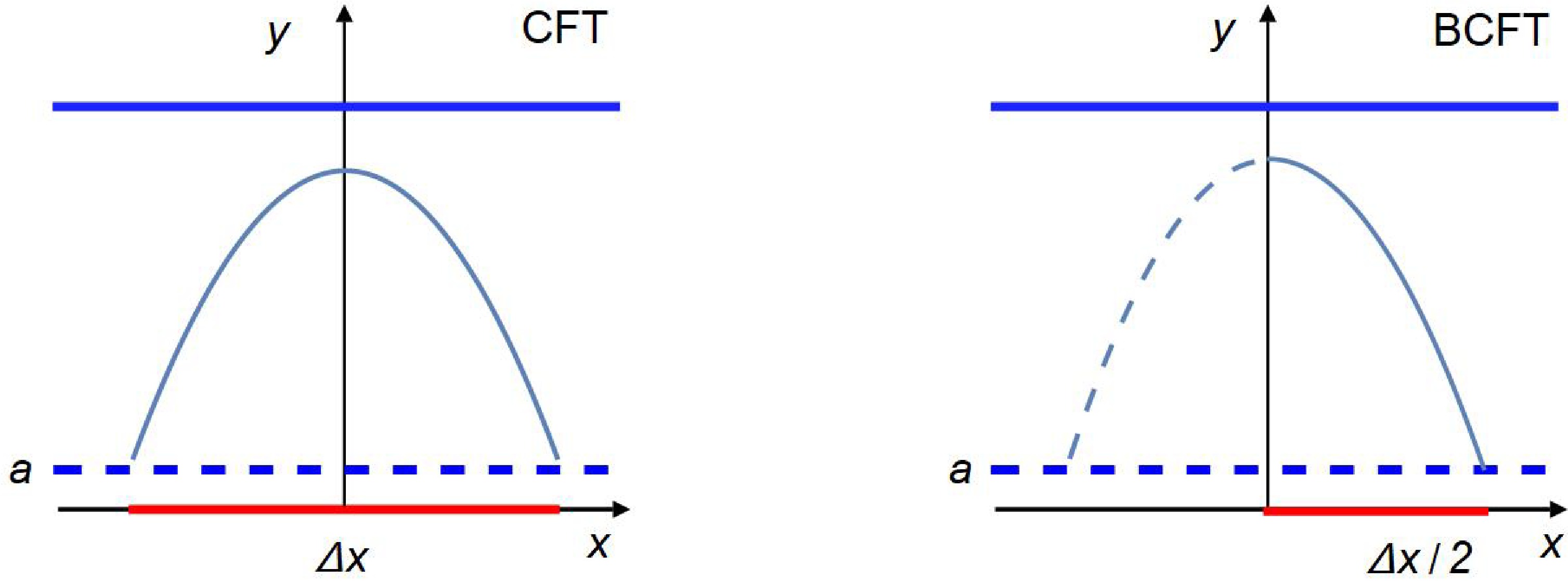

Figure 1.  (color online) The left-hand side image shows the geodesic identified from CFT EE. The endpoints are fixed at $y=y^{\prime}=a$. The solid curve in the right-hand side image represents the geodesic identified from the BCFT EE. The endpoints are fixed at $y=a$ and $y'=\beta_{H}$, and the entangling length is $\Delta x/2$.

In contrast, by using the general expression of the geodesic length (30), we have two other methods of calculating the length of this geodesic. The first method is to straightforwardly substitute $y=a$, $y'=\beta_{H}$, and $\Delta x/2\to\infty$ into (30) to obtain

We easily understand that this length is half the geodesic length connecting $y=y^{\prime}=a$ and $\Delta x\to\infty$. Therefore, the second method is

These three lengths in Eq. (36), (37), and (38) must be identical, as shown in Fig. 2. Thus, we obtain

Figure 2.  (color online) The left-hand image is given by the BCFT. The middle image is obtained from $L_{\rm{bulk}}$ by setting $y=a$, $y^{\prime}=\beta_{H}$ and $\triangle x/2\rightarrow \infty$. The right-hand image is also given by $L_{\rm{bulk}}$ from a different perspective, by setting $y=y^{\prime}=a$ and $\Delta x\to\infty$. The solid lines in all the three pictures describe the same object.

The derivation of this constraint does not require $\beta_{H}\gg a$. As long as $\beta_{H}$ is the upper bound of y, the derivation is justified. Because a is a varying cut-off not beyond $\beta_{H}$, satisfying $0<a/\beta_{H}\le1,$ we can safely replace $\dfrac{a}{\beta_{H}}$ by $\dfrac{y}{\beta_{H}}$ to obtain

Step 5: An important lesson we learn from the free CFT₂ case is that, to completely determine the dual geometry, we must know the geodesic length between a and $\beta_{H}$ with $\triangle x=0$, i.e., the vertical geodesic. To be consistent, this particular geodesic length must be provided by the CFT₂ EE. In the free CFT₂, the IR EE precisely fits the requirement. The finite temperature CFT₂ does not have such IR EE.

Remarkably, we know that the finite temperature CFT₂ and finite size CFT₂ have the same geometry ${\mathbb R}\times {\bf S}^1$. We can either interpret it as a CFT on a compact spatial interval of size $L_S$ or as a thermal CFT on the real line with the Euclidean time along the circle with the period $\beta = L_S$, as explained in [5, 13] in detail. Therefore, two CFTs are basically the same scenario and have the same bulk dual. We are allowed to use the results from both CFTs to construct the dual bulk geometry with the identification Therefore, we map the finite temperature system to a finite size ($L_{S}$) system by replacing $\beta\rightarrow L_{S}$ and impose the periodic boundary condition ¹

Therefore, the geodesic length between a and $\beta_{H}=\dfrac{\beta}{2\pi}$ in the finite temperature system equals the one that connects a and $\dfrac{L}{2\pi}$ in the finite size system:

Noting that $\dfrac{L_{S}}{2\pi}$ is the radius of the finite size system with the circumference $L_{S}$, this geodesic extends from boundary to the center of the circle, as shown in Fig. 3.

Figure 3.  (color online) Geodesic between $y=a$ and $y^{\prime}=\beta_{H}$ at a finite temperature system mapped to a finite size system, corresponding the radius of a circle from $y=a$ to $y=\dfrac{L}{2\pi}$.

We know that the EE of a finite size system is

The maximal EE is achieved by splitting the circle into two equal regions, $\Delta x=L_{S}/2$. The corresponding geodesic is simply a diameter

Thus, we can obtain the value we desire:

We now map $L_{S}\to\beta$ to obtain the geodesic length between a and $\beta_{H}=\dfrac{\beta}{2\pi}$ in the finite temperature system:

Therefore, from the general expression (30), as $x=x^{\prime}$, $t=t^{\prime}$, $y=a$, and $y^{\prime}=\beta_{H}$, we obtain

Thus, we obtain

For convenience, we summarize all the constraints we have obtained for the general expression (30) of the geodesic length:

From Eqs. (50) and (52), we obtain

Because a is a varying quantity, y or $y'=\beta_{H}$ must be a zero of $g(y/\beta_{H},y'/\beta_{H})$. Moreover, g must be symmetric for y and $y'$. Therefore, the function form must be

Moreover, from Eqs. (50) and (51), we obtain

Thus, we can easily fix $n=2$ and $\kappa=1/2$ and

Similarly, from Eq. (50), we obtain

where m, $\delta>0$ are some numbers.

The story is not over yet. To match Eq. (49), we must have $\sigma_{1}=\theta_{1}$. When applying Eq. (1) to calculate the metric, noting that a limit $\Delta x,\;\Delta y,\;\Delta t\to0$ will be imposed after making the derivatives, we easily obsevre that the terms proportional to $\left(\dfrac{\Delta y}{\beta_{H}}\right)^{2}$ contribute only to $g_{yy}$ but not to $g_{xx}$ and $g_{tt}$. Therefore, based on Eqs. (56) and (57), without altering the derived metric, equivalently, we are free to pack all the corrections into $g(y,y')$ and simply set $f(y,y')=1$. Finally, we obtain

Applying (1), we obtain the metric of the BTZ black hole:

Because the finite size system has the same topology as the finite temperature one, a simple method of fixing the leading behavior of the dual geometry of the finite size system is to use the transformation $\beta=-{\rm i}L$, which leads to the pure AdS₃ in the global coordinate. Similarly, we can fix the leading behaviors of the dual geometries of CFT₂ with topological defects under transformation $\beta=-{\rm i}L/\gamma_{\text{con}}$.

In this final section, we discuss our results and provide several inspirations as well as conjectures. In summary, we have demonstrated an approach to fixing the leading behaviors of three dimensional dual geometries, such as asymptotic AdS₃ and BTZ black holes, from the EEs of $\text{CFT}_{2}$. Our derivation relies only on the holographic principle without any assumptions about AdS/CFT and bulk geometry. The steps of the method are as follows:

1. Identify the energy cut-off as an extra dimension.

2. Identify the EE with the geodesic length of the unknown dual geometry. The geodesics are attached on the boundary.

3. Write down the bulk geodesic length by making the most general extension of the geodesic ending on boundary to include the extra dimension.

4. Use properties a geodesic must respect, say, zero length for coincide endpoints, to impose constraints on the bulk geodesic function form.

5. Use the IR-like EE representing a geodesic whose one endpoint stands on the boundary and another stretches into the bulk of the unknown geometry, to restrict the bulk geodesic function form.

6. Apply Eq. (1) to fix the leading behavior of the metric.

Our approach, from the derivation of the BTZ black hole, may apply for all the three dimensional geometries. As we have explained, because they have the same topology as the finite temperature CFT₂, the finite size CFT₂ and CFT₂ with topological defects can be easily determined by using simple transformations, although an independent parallel derivation is desirable. Basically, we need only consider one representative for each topology. Therefore, the next non-trivial steps involve investigating the chiral CFT₂ or finite size thermal CFT₂. Probably, the only obstacle is to determine the IR-like EEs from the CFT side. The existence of the IR-like EEs is unquestionable, but it might be difficult to calculate from the CFT side. A compromise is to borrow the IR-like EEs from holographic calculation, if not so strict. For CFT living on surfaces beyond the torus, we believe the derivation can still be performed, but we must know the EEs, both UV and IR-like, which are difficult to obtain from the CFT side. In addition, it would be of significant interest to consider the CFT₂ which are dual to sourced gravity. We may learn more non-trivial things from these examples.

Our derivation shows that the bulk geometry cannot be determined using UV EE only. For a higher dimensional case $d+1>3$, the scenario is complicated. One reason is that no method is available to calculate the metric from minimal surfaces. Another challenge is that even for a single topology, many inequivalent gravitational structures exist in higher dimensions. We are not certain if other subtleties will occur.

An interesting question is, Is it necessary to identify the EE with the geodesic to fix the leading behavior of the metric? The answer appears to be negative. As we know, the arguments of the EE include both spacetime directions t, x as well as the energy cut-offs such as a, ξ, β, .... After identifying the energy scale as an extra dimension y, we canintroduce a generalized EE ${\cal{S}}_{\rm EE} \left(t,\;t';\;x,\;x';\;y,\;y'\right)$ as follows:

• We denote the energy generated dimension as y. Therefore, the energy cut-offs are different values on the dimension y.

• Because y is on the same footing as the ordinary spacetime directions x, t, it is natural to generalize $S_{\rm EE}(t,t';x,x';a,\beta,\cdots)$ to ${\cal{S}}_{\rm EE}\left(t,t';x,x';y,y'\right)$ in the most generic manner.

$\Longrightarrow$This step corresponds to extending the boundary attached geodesic to the bulk geodesic.

• Under various limits, the generalized EE ${\cal{S}}_{\rm EE}\left(t,t';x,x';y,y'\right)$ should reproduce all the EEs of a specified CFT, such as the UV or IR-like EEs.

$\Longrightarrow$This step corresponds to using various EEs to determine the behaviors of the regular functions in our approach.

• The generalized EE ${\cal{S}}_{\rm EE} \left(t,t';x,x';y,y'\right)$ should be renormalized because the infinities of QFT are caused by energy, which is now a new dimension.

$\Longrightarrow$ This step corresponds to demanding the vanished geodesic length for coincident endpoints and other consistencies.

Therefore, our previous calculations naturally fit the procedure. Now, we immediately have an interesting equation:

All the derivations in this paper can be expressed in this pattern. Consequently, all GR quantities, such as the connection, Riemann tensor, etc., can be subsequently constructed. This equation indicates some new interpretations:

• Spacetime is not an emergent structure from quantum entanglement, but it is quantum entanglement itself, simply viewed from a different angle.

• Quantum entanglement with different lengths knits the spacetime.

Moreover, we wish to clarify two significant reasons for our derivations appearing heavy:

1. The advantages of our method is to also cover the time-like direction of the spacetime metric naturally. This is very difficult because we know only the information of the lower dimensional theories.

2. Our objective is to determine not only the linear order but also the singularity and event horizon of BTZ spacetime. The behaviors of black hole's singularity and event horizon cannot be extracted using the leading term of the spacetime metric directly. This is why we use more results of EEs and aim to fix more accurate leading behaviors of bulk geometries.

Therefore, in this paper, our aim is not to explain how the bulk geometry emerges from EEs or to derive the bulk dynamics (Einstein's equation) from the boundary theory, but only to show that the EEs of $\text{CFT}_{2}$ are sufficient to fix the leading behaviors of the bulk spacetime geometries.

Another point deserves a special emphasis. Our results demonstrate that when we treat the energy scale as a usual space-like dimension, the CFT contains almost all the classical information of the dual geometry, at least for $d=2$. In AdS/CFT correspondence, to compare the correlation functions of the dual theories, we take limits to push the AdS$_{d+1}$ bulk-to-bulk correlation function onto the boundary and then match the CFT$_{d}$ correlation function [17]. However, the method of lifting the CFT$_{d}$ correlation function into the bulk directly is still an open question. Our derivations show that when we treat the energy scale as an extra dimension, after imposing some consistent constraints, the bulk-to-bulk correlation function from the boundary-to-boundary one can be derived. Thinking it over, we observe that two equations govern the dynamics of operators in QFT: the Callan-Symanzik (RG) equation and equation of motion (EOM). The RG equation informs us how the operators evolve with respect to energy scales. The EOM determines the evolution of the operators with respect to spacetime coordinates. Therefore, logically, we can naturally conjecture that

which implies a unification of the RG equation and field EOM.

We are deeply indebted to Bo Ning for many illuminating discussions and suggestions. We are also very grateful to Q. Gan, S. Kim, J. Lu, H. Nakajima, S. Ying, and S. He for very helpful discussions and suggestions.