


 Abstract
 HTML
HTML Reference
 Related
 PDF
PDF


-
The 125 GeV Higgs was discovered at the LHC [1, 2] with the correct spin and CP property, and production rates that are globally consistent with the Standard Model (SM), according to both the ATLAS and CMS collaborations [3-7]. In view of the deviations in the Higgs production rates, there is still a possibility for new physics, such as different symmetry-breaking mechanisms, new particles in the Higgs coupling loops, or Higgs mixing with additional scalars. After the Higgs discovery, whether an additional scalar exists is a natural question that most experimentalists and theorists are concerned with.
However, we do not exactly know the physics beyond the SM even in the low mass region. Before LHC, the largest center-of-mass energy was 209 GeV at LEP, which excluded an SM-like Higgs below 114.4 GeV [8]. In fact, the data set from LEP is so small that a light scalar could still be possible, with production rates below the SM prediction. For example, recently the CMS collaboration presented their search for new low-mass resonances decaying into two photons, both for 8 TeV and 13 TeV data sets, and a small excess around 95 GeV was hinted at, with approximately 2.8
$\sigma$ local (1.3$\sigma$ global) significance for a hypothetical mass of 95.3 GeV in the combined analysis [9]. The signal around 95 GeV at the 13 TeV LHC is about$\sigma^{13{\rm TeV}}_{\gamma\gamma}\approx80\pm20$ fb, or$\sigma^{13{\rm TeV}}_{\gamma\gamma}/ $ ${\rm SM}\approx $ $0.64\pm0.16$ . Such a result was interpreted or discussed in several papers [10-32]. For the same mass region and the same channel, the ATLAS collaboration released their new search result with about$80$ fb−1 of data at 13 TeV, but no excess was observed, with an exclusion limit of$\sigma^{13{\rm TeV}}_{\gamma\gamma}\lesssim60$ fb (fiducial) at 95% confidence level (CL) [33]. Compared to the CMS result, the ATLAS signal around 95 GeV at the 13 TeV LHC is about$\sigma^{13{\rm TeV}}_{\gamma\gamma}\approx18\pm18$ fb (fiducial), or$\sigma^{13{\rm TeV}}_{\gamma\gamma}/{\rm SM}\approx0.14\pm0.14$ . Considering the difference between these two collaborations, further searches at the LHC or at future colliders are necessary. The difference between these two collaborations, together with the other small excesses seen at 98 GeV [8], 28 GeV [34] and 115 GeV [35], reflects our uncertainty in the physics beyond the SM in the low mass region. Thus, it is still interesting to consider a light scalar in new physics models, which could have different diphoton rates in different parameter spaces, and could help interpret the results of the two LHC collaborations, and help distinguish the parameter spaces at the LHC and at future colliders.In this letter, we consider the Minimal Dilaton Model (MDM), which extends the SM by a dilaton-like singlet scalar and vector-like fermions [36-41]. Just like the traditional dilaton [42-48], the singlet scalar in this model arises from a strong interaction theory with approximate scale invariance at a certain high energy scale, whose breakdown triggers the electroweak symmetry breaking. The singlet, as the pseudo Nambu-Goldstone particle of the broken invariance, can be naturally light compared with the high energy scale. Unlike the traditional dilaton theory, this model assumes that only the Higgs and top quark sectors, and not all SM particles, can interact with the dynamics sector, and consequently that the singlet does not couple directly to the fermions and
$W$ ,$Z$ bosons in the SM. Meanwhile, the additional vector-like fermions act as the lightest particles in the dynamics sector, to which the singlet naturally couples in order to recover the scale invariance:$M \to M e^{-\phi/f}$ . As a result, these fermions can induce interactions between a pure singlet and photons/gluons, or Z/W boson with loop effect. Furthermore, mixing with the SM Higgs field can also induce interactions. Thus, a light scalar can exist in MDM, mixed with the SM Higgs and singlet fields, and could be further studied at the LHC or at future electron-positron colliders. Due to the limited space in this letter, we leave that study for our future work.This letter is organized as follows. We first briefly introduce the MDM in Section 2. In Section 3, we give the formulas for production rates of MDM scalars at the LHC. In Section 4, we discuss the constraints applied in the model, and show the calculations and results. Finally, we draw our conclusions in Section 5.
-
As introduced in Sec. 1, MDM extends the SM by a dilaton-like singlet field
$S$ and a vector-like top partner field$T$ . The effective Lagrangian can be written as [36, 37]$ \begin{split} \mathcal L = & \mathcal L_{\rm SM} -\frac{1}{2}\partial_\mu S\partial^\mu S -\tilde V(S, H)\\ & -\overline T\left({\not \!\!\!D} +\frac{M}{f}S\right)T -\left[y'\overline T_R(q_{3L}\cdot H)+{\rm h.c.}\right], \end{split} $

(1) where
$q_{3L}$ ,$M$ and$\mathcal L_{\rm SM}$ are the third-generation quark doublet, the strong-dynamics scale, and the SM Lagrangian without the Higgs potential, respectively. The new scalar potential$\tilde{V}(S, H)$ is in general given by$ \begin{split} \tilde V(S, H) = & M_H^2|H|^2+\frac{M_S^2}{2}S^2+\frac{\kappa}{2}S^2|H|^2 \\ & +\frac{\lambda_H}{4}|H|^4+\frac{\lambda_S}{24}S^4, \end{split} $

(2) with
$M_H$ ,$M_S$ ,$\kappa$ ,$\lambda_H$ , and$\lambda_S$ as free parameters. To break the symmetries,$H$ and$S$ get vacuum expectation values (VEVs)$v=246$ GeV and$f$ , respectively. The singlet dilaton field$S$ can mix with the CP-even Higgs component$H^0$ , forming two mass eigenstates$h, s$ , that is$ \begin{align} \left[ \begin{array}{c} h \\ s \end{array} \right] = \left[ \begin{array}{cc} \cos\theta_S & \sin\theta_S \\ -\sin\theta_S & \cos\theta_S \end{array} \right] \left[ \begin{array}{c} H^0-\displaystyle\frac{v}{\sqrt{2}}\\ S-f \end{array} \right]. \end{align} $

(3) In this work we fix
$m_h= 125.09$ GeV, which is the combined mass value of the ATLAS and CMS collaborations [49]. For convenience we express$\lambda_H$ ,$\lambda_S$ and$\kappa$ by input parameters$f$ ,$v$ ,$\theta_S$ ,$m_h$ and$m_s$ , and define [36, 37]$ \begin{align} \eta & \equiv & \frac{v}{f} N_T , \end{align} $

(4) where
$N_T$ is the number of fields$T$ , which we set to 1 in this work. With the conditions$m_{t'}\gg m_t$ and$\tan\theta_L\ll m_{t'}/m_t$ , the normalized couplings of$h$ and$s$ are given by [36, 37]$ \begin{split} &C_{hVV}/{\rm SM} = C_{hff}/{\rm SM} = \cos\theta_S, \\ &C_{sVV}/{\rm SM} = C_{sff}/{\rm SM} = -\sin\theta_S, \end{split} $

(5) where
$V$ denotes either$W^{\pm}$ or$Z$ boson, and$f$ the fermions, except for the top quark sector.The new fermion fields
$(T_L, T_R)$ have the same quantum numbers as the SM fields$(q_{3L}, u_{3R})$ , thus they mix to form two mass eigenstates$(t, t')$ , that is$ \begin{align} \left[ \begin{array}{c} t_L \\ t'_L \end{array} \right] = V_L^{\dagger} \left[ \begin{array}{c} q_{3L} \\ T_L \end{array} \right], \qquad \left[ \begin{array}{c} t_R \\ t'_R \end{array} \right] = V_R^{\dagger} \left[ \begin{array}{c} u_{3R} \\ T_R \end{array} \right], \end{align} $

(6) where we chose the mixing matrices as
$ \begin{align} V_L = \left[ \begin{array}{cc} \cos\theta_L & \sin\theta_L \\ -\sin\theta_L & \cos\theta_L \end{array}\right] , \; V_R = \left[ \begin{array}{cc} \cos\theta_R & \sin\theta_R \\ -\sin\theta_R & \cos\theta_R \end{array}\right]. \end{align} $

(7) From Eq. (1), the mixing mass matrix is
$ \begin{align} M_t= \left[\begin{array}{cc}\displaystyle\frac{v}{\sqrt{2}} y_t &\displaystyle\frac{v}{\sqrt{2}} y' \\ 0 & f y_s \end{array} \right], \end{align} $

(8) which can be diagonalized as
$ \begin{align} V_L^{\dagger} M_t V_{R} = \left[ \begin{array}{cc} m_t & 0 \\0 & m_{t'} \end{array} \right]. \end{align} $

(9) Choosing
$m_t, m_{t'}, \theta_L$ as input parameters, the other parameters can be expressed as$ \begin{split} \tan\theta_R = & \frac{m_t}{m_{t'}}\tan\theta_L, \\ y_t = & \frac{\sqrt{2}}{v}(m_t \cos\theta_L \cos\theta_R +m_{t'} \sin\theta_L \sin\theta_R)\\ = & \frac{\sqrt{2}}{v}\frac{m_t m_{t'}}{\sqrt{m_t^2 \sin^2\theta_L +m_{t'}\cos^2\theta_L}}, \\ y' = & \frac{\sqrt{2}}{v}(-m_t \cos\theta_L \sin\theta_R +m_{t'} \sin\theta_L \cos\theta_R)\\ = & \frac{\sqrt{2}}{v}\frac{(m_{t'}^2 -m_t^2) \cos\theta_L \sin\theta_L}{\sqrt{m_t^2 \sin^2\theta_L +m_{t'}\cos^2\theta_L}}, \\ y_s= & \frac{1}{f} \sqrt{m_t^2 \sin\theta_L^2 +m_{t'}\cos^2\theta_L} ~. \end{split} $

(10) Since gluon/photon can only couple to a pair of the same mass eigenstates
$t$ or$t'$ at tree level, in the calculations of loop-induced coupling of scalars to$gg/\gamma\gamma$ , we can normalize the Yukawa couplings of scalars to top quark sector to their SM values$ \begin{split} C_{ht\bar{t}}/{\rm SM} = & \cos^2\theta_L\cos\theta_S +\eta\sin^2\theta_L\sin\theta_S, \\ C_{ht'\bar{t'}}/{\rm SM} = & \sin^2\theta_L\cos\theta_S +\eta\cos^2\theta_L\sin\theta_S, \\ C_{st\bar{t}}/{\rm SM} = & -\cos^2\theta_L\sin\theta_S +\eta\sin^2\theta_L\cos\theta_S, \\ C_{st'\bar{t'}}/{\rm SM} = & -\sin^2\theta_L\sin\theta_S +\eta\cos^2\theta_L\cos\theta_S, \end{split} $

(11) while we should know the new couplings of
$h$ ,$s$ and$Z$ to a pair of different mass eigenstates$t$ and$t'$ . With Eqs. (5) and (11), we can get the normalized loop-induced couplings$ \begin{split} C_{hgg}/{\rm SM} =& \cos\theta_S +\eta\sin\theta_S, \\ C_{h\gamma\gamma}/{\rm SM} =&\cos\theta_S -0.27\times\eta\sin\theta_S, \\ C_{sgg}/{\rm SM} =& \left[-A_b \sin\theta_S \!+\!A_t \times \left(-\cos^2\theta_L\sin\theta_S \!+\!\eta\sin^2\theta_L\cos\theta_S\right)\right. \\ &\!+\!A_{t'} \!\times\! \left.\left(-\sin^2\theta_L\sin\theta_S \!+\!\eta\cos^2\theta_L\cos\theta_S\right)\right] \! /\!(A_t\!+\!A_b), \end{split} $

$ \begin{split} C_{s\gamma\gamma}/{\rm SM} =& \left[-\left(A_W+\frac{1}{3}A_b\right) \times \sin\theta_S \right.+\frac{4}{3}A_t\\ & \times \left(-\cos^2\theta_L\sin\theta_S +\eta\sin^2\theta_L\cos\theta_S\right)+\frac{4}{3}A_{t'} \\ &\left. \times \left(-\sin^2\theta_L\sin\theta_S +\eta\cos^2\theta_L\cos\theta_S\right)\right] \\ &\left/\left[A_W+\frac{4}{3}A_t+\frac{1}{3}A_b\right]\right., \end{split} $

(12) where
$A_i$ is the loop function presented in Ref. [50] with particle$i$ running in the loop. When$m_s=95$ GeV, the loop-induced coupling$sgg, s\gamma\gamma$ can be approximated by$ \begin{split} C_{sgg}/{\rm SM} \simeq& -\sin\theta_S +\eta\cos\theta_S, \\ C_{s\gamma\gamma}/{\rm SM} \simeq& -\sin\theta_S -0.31\eta\cos\theta_S. \end{split} $

(13) -
In MDM, we assumed
$h$ as the 125 GeV Higgs. Since the current data for the Higgs production rates are globally very close to the SM Higgs, the mixing angle$\theta_S$ between Higgs and dilaton can be very small [38]. In this work, we consider the dilaton-like scalar$s$ to be lighter, e.g.,$65\sim122$ GeV, which is constrained by the low mass resonance searches at the LHC①); or 95 GeV, corresponding to the low-mass resonance suspected by the CMS collaboration. Furthermore, we suggest further searches of the light scalar at the LHC and at future electron-positron colliders. The lighter scalar with a mass of about 95 GeV and small$\theta_S$ could be expected to decay mainly into$gg$ ,$\gamma \gamma$ ,$f \bar{f}$ (such as$b \bar{b}$ ,$c \bar{c}$ , and$\tau^+\tau^-$ ) [51]. In this section, we list the formulae used for the production and decay of the two scalars.First, we list the decay and production information for the SM Higgs at 125 and 95 GeV, which are taken from Ref. [51]. In Table 1, we list the branching ratios and the total width. In Table 2, we list the cross sections at the 13 TeV LHC, which are calculated at NNLO level.
MH /GeV ${b\bar{b}}$ 

${c\bar{c}}$ 

${\tau^+\tau^-}$ 

WW* ZZ* gg ${\gamma\gamma}$ 

${\Gamma^{\rm SM}_{\rm tot}}$ /MeV

125.0 0.591 0.0289 0.0635 0.208 0.0262 0.0782 0.00231 4.07 95.0 0.810 0.0397 0.0824 0.00451 0.000651 0.0608 0.00141 2.38 Table 1. The decay branching ratios and the total width of the SM Higgs at 125 and 95 GeV [51].
${M_H}$ /GeV

${\sigma^{\rm SM}_{\rm ggF}}$ /pb

${\sigma^{\rm SM}_{VBF}}$ /pb

${\sigma^{\rm SM}_{WH}}$ /pb

${\sigma^{\rm SM}_{ZH}}$ /pb

${\sigma^{\rm SM}_{Ht\bar{t}}}$ /pb

125.0 43.92 3.748 1.380 0.8696 0.5085 95.0 70.64 3.680 2.931 1.622 0.5349 Table 2. The production cross sections at the 13 TeV LHC of the SM Higgs at 125 and 95 GeV [51].
With the decay information for the SM Higgs, the total width and branching ratios of the scalars
$\phi=h, s$ in MDM can be written as$ \begin{align} \Gamma_{\rm tot}^{\phi} = & \Gamma^{\rm SM}_{\rm tot} \times \sum_{xx} \left[ Br^{\rm SM}_{\phi\to xx} \times |C_{\phi xx}/{\rm SM}|^2 \right], \end{align} $

(14) $ \begin{align} Br_{\phi\to xx} = & Br^{\rm SM}_{\phi\to xx} \times |C_{\phi xx}/{\rm SM}|^2 \times \frac{\Gamma^{\rm SM}_{\rm tot}}{\Gamma_{\rm tot}^{\phi}}, \end{align} $

(15) where
$xx=b\bar{b}, c\bar{c}, \tau^+\tau^-, $ WW*, ZZ*, gg,$\gamma\gamma $ , and$C_{\phi xx}/{\rm SM}$ are the corresponding normalized Yukawa couplings at leading order defined in Eqs. (5), (11) and (12).With the production information for the SM Higgs, the production rates of the scalars
$\phi=h, s$ in MDM at the 13 TeV LHC can be calculated as$ \sigma_{ggF} = \sigma^{\rm SM}_{ggF}(m_\phi) \times |C_{\phi gg}/{\rm SM}|^2, $

(16) $ \sigma_{{\rm VBF}, V\phi} = \sigma^{\rm SM}_{\rm VBF, VH}(m_\phi) \times |C_{\phi VV}/{\rm SM}|^2, $

(17) $ \sigma_{\phi t\bar{t}} = \sigma^{\rm SM}_{H t\bar{t}}(m_\phi) \times |C_{\phi t\bar{t}}/{\rm SM}|^2, $

(18) where
$C_{\phi xx}/{\rm SM}$ with$xx=gg, WW, ZZ, t\bar{t}$ , are also the corresponding normalized Yukawa couplings at leading order, defined in Eqs.(12), (5), and (11).From the formulas and information above, one can draw the following important conclusions:
● If
$|\tan\theta_S| \gg \eta/4$ , the dominant decay branching ratio of the 95 GeV scalar is$s\to b\bar{b}$ , and thus its total width and main decay branching ratios are$ \begin{split} \Gamma_{\rm tot}^{s} \simeq& 2.4 |\sin\theta_S|^2 {\rm ~MeV}, \\ Br_{s\to b\bar{b}} \simeq& 0.8, \\ Br_{s\to gg} \simeq& 0.06, \\ Br_{s\to \gamma\gamma} \simeq& 0.0014, \end{split} $

(19) where the branching ratio of diphoton can be slightly larger (smaller) when
$\tan\theta_S$ is positive (negative).● If
$|\tan\theta_S| \ll \eta/4$ , the dominant decay branching ratio of the 95 GeV scalar is$s\to gg$ , and thus its total width and main decay branching ratios are$ \begin{split} \Gamma_{\rm tot}^{s} \simeq& 0.15 \eta^2 {\rm ~MeV}, \\ Br_{s\to gg} \simeq& 1, \\ Br_{s\to \gamma\gamma} \simeq& 0.0022, \end{split} $

(20) where the branching ratio of diphoton can be slightly larger (smaller) when the small
$\tan\theta_S$ is positive (negative).● If
$|\tan\theta_S|$ or$|\sin\theta_S|$ is small, the production rate of$s$ at the LHC is proportional to$\eta^2$ . Thus the golden probing channel for light dilaton at the LHC is$gg\to s \to \gamma\gamma$ , whose cross section can be approximated by$ \begin{align} \sigma_{\gamma \gamma} (m_s) \simeq& \eta^2 \times \sigma^{\rm SM}_{\rm ggF}(m_s) \times Br_{s\to\gamma\gamma}, \end{align} $

(21) ● If
$|\sin\theta_S|$ or$|\tan\theta_S|$ is not small, the vector bosons fusion (VBF) and vector boson scalar strahlung (Vs) production rates are significant at tree level, and$s\to b\bar{b}$ with$s$ produced through VBF or Vs can be used as another channel at the LHC, whose cross section can be approximated by$ \begin{split} \sigma_{{\rm VBF}, b\bar{b}} (m_s) \simeq& |\sin\theta_S|^2 \times \sigma^{\rm SM}_{\rm VBF}(m_s) \times Br_{s\to b\bar{b}} , \\ \sigma_{{\rm Vs}, b\bar{b}} (m_s) \simeq& |\sin\theta_S|^2 \times \sigma^{\rm SM}_{\rm VH}(m_s) \times Br_{s\to b\bar{b}} . \end{split} $

(22) In this case, it can also be studied at future electron-positron colliders.
● If
$|\sin\theta_S|\approx0$ , the loop effect of$t/t'$ in the effective coupling of$sZZ$ may be non-ignorable [52-56]. We leave this study for our future work. -
In this section, we first scan over the parameter space of MDM under various experimental constraints. Then for the selected samples, we investigate the features of
$h$ and$s$ . Before our scan, we would like to clarify the following facts● Firstly, since the character of dilaton in MDM differs greatly from the SM Higgs boson, its mass may vary from several GeV to several hundred GeV without conflicting with the LEP and LHC data in search for the Higgs boson. In fact, both ATLAS and CMS released their search results for low mass resonances in the region of 65-122 GeV at the LHC [9, 33, 57, 58].
● Secondly, since the diphoton rate of the light scalar is constrained by the LHC data,
$\eta\equiv v/f$ cannot be very large. Thus we take$0 <\eta\leqslant 10$ , and pay special attention in our study to the case$\eta < 1$ .● Thirdly, although in principle
$\theta_S$ may vary from$-\pi/2$ to$\pi/2$ , the Higgs data require that it be around zero so that$h$ is mainly responsible for the electroweak symmetry breaking. In practice, requiring$|\tan\theta_S| \leqslant 2$ will suffice.● Finally, in MDM
$t'$ may decay into$th, ts, tZ, bW$ at tree level. With$36$ fb-1 of data at the 13 TeV LHC, the combined analyses of$t'\to tH, tZ, bW$ by ATLAS excluded a vector-like$t'$ below 1.31 TeV at$95\%$ CL [59-61]. The CMS data exclude$t'$ with masses below 1140-1300 GeV [62-64]. The perturbability may also require$t'$ not to be too heavy.With the above considerations, we first scan the following parameter space:
$ \begin{split} & 0.01< \eta <10, ~~~~ |\tan\theta_S|<2, ~~~~ 0< |\sin\theta_L| <1, \\ & 65 <m_s< 122~{\rm GeV}, ~~~~ 1 <m_{t'}< 100~{\rm TeV}. \end{split} $

(23) In our scan, we consider the following theoretical and experimental constraints:
(1) Theoretical constraint of vacuum stability for the scalar potential, which corresponds to the requirement
$4 \lambda_H \lambda_S - \lambda_{HS}^2 >0$ [36].(2) Theoretical constraints of perturbability for scalar couplings
$\lambda_S, \lambda_H, \kappa < 4 \pi$ and Yukawa couplings$y_t, y', y_s < $ $4 \pi $ .(3) Theoretical constraints from requirement that no Landau pole exists below 1 TeV. For parameter running, we use the renormalization group equations (RGE) of the three scalar coupling parameters which are derived with SARAH-4.12.3 [65-67],
$ \begin{split} {\mathcal D} \equiv & 16 \pi^2 \mu \frac{d}{d Q}, \\ {\mathcal D} \lambda_H = & 6 \lambda_H^2 +2\kappa^2, \\ {\mathcal D} \lambda_S = & 3 \lambda_S^2 +12\kappa^2, \\ {\mathcal D} \kappa = & \kappa (3\lambda_H + \lambda_S) +4\kappa^2, \end{split} $

(24) (4) Experimental constraints from the electroweak precision data (EWPD). We calculate the Peskin-Takeuchi
$S$ and$T$ parameters [68] with the formulae presented in [36], and construct$\chi^2_{ST}$ by the following experimental fit results with$m_{h, \rm{ref}}=125$ GeV and$m_{t, \rm{ref}}=173$ GeV [69]:$ \begin{align} S=0.02\pm0.07, ~~ T=0.06\pm0.06, ~~ \rho_{ST}=0.92. \end{align} $

(25) In our calculation, we require that the samples satisfy
$\chi^2_{ST} \leqslant 6.18$ ②). We do not consider the constraints from$V_{tb}$ and$R_b$ since they are weaker than those for the$S, T$ parameters [36].(5) Experimental constraints from the LEP, Tevatron and LHC searches for Higgs-like resonances. We implement these constraints with the package HiggsBounds— 5.2.0beta [70]. For the case we are considering in this work (
$65<m_s<122$ GeV, cross section and decay calculated at leading order), the main constraints to the light scalar come from diphoton results at the LHC [9, 33, 57, 58], and the$Zb\bar{b}$ channel at LEP [8]②).6) Experimental constraints from the 125 GeV Higgs data at LHC Run I and Run II. We first use the method from our former work [38, 74], with Higgs data updated with Fig. 3 in [75] and Fig. 5 left in [76]. There are 20 experimental data sets in total, so we require
$\chi^2_{20}\leqslant 31.4$ , which means that each selected sample fits 20 experimental data sets at 95% CL②). We then use HiggsSignal-2.2.0beta [77] , which includes both Run I and Run II data. We require$\chi^2_{117}<143.2$ , which means that either the P value for Higgs data$P_h>0.05$ , or that each selected sample fits all 117 experimental data sets at 95% CL.With samples satisfying all constraints listed above, we analyze the parameters, couplings and production rates of the scalars.
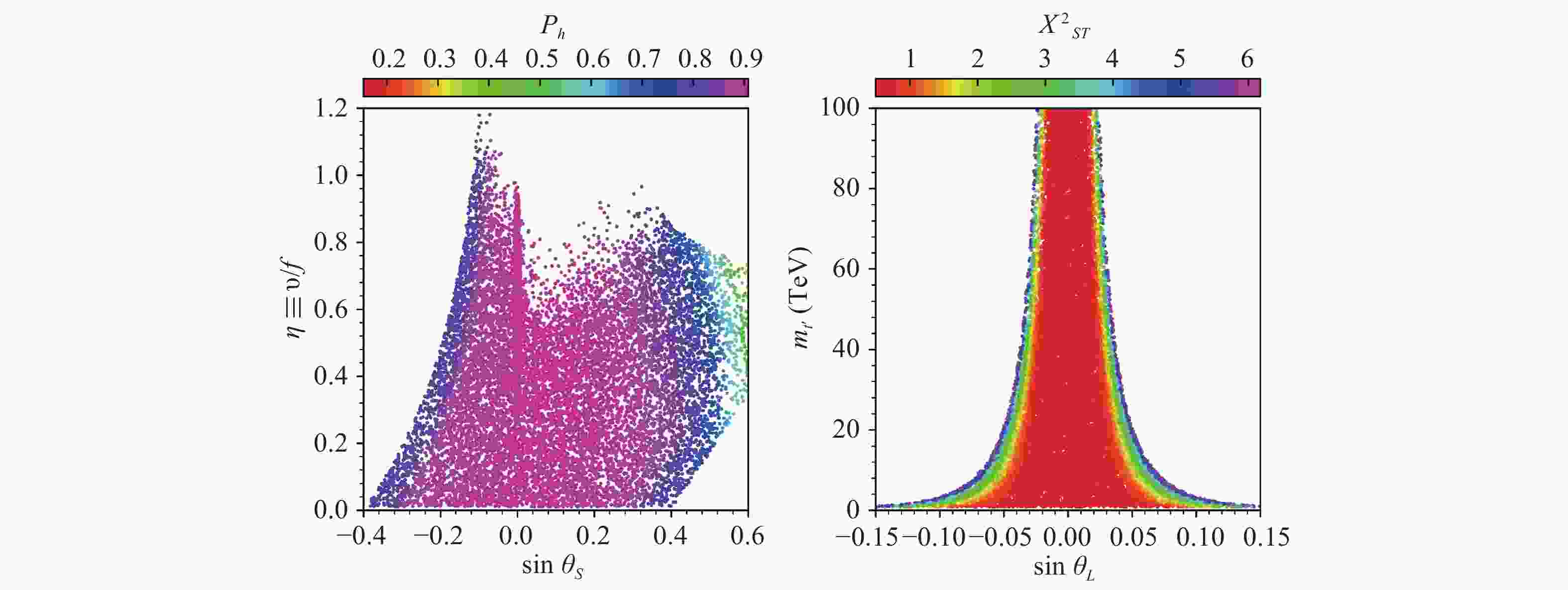
In Fig. 1, we project the selected data samples on the planes of
$\eta \equiv v/f$ versus$\sin\theta_S$ (left), and$m_{t'}$ versus$\sin\theta_L$ (right). The colors indicate$P_h$ (left) and$\chi^2_{ST}$ (right), where$P_h$ is the P value calculated with the latest LHC Run I and Run II Higgs data in HiggsSignal-2.2.0, and$\chi^2_{ST}$ is the$\chi^2$ in EWPD fit of the parameters$S$ and$T$ . From the figure we can see that:● Our strategy for the Higgs fit is complementary with that of HiggsSignal. Samples with
$0.05<P_h\lesssim0.2$ are excluded by our strategy, while we checked that samples with$22\lesssim{\chi'}^2_h<31.4$ (or$0.05<P'_h\lesssim0.5$ ) in our strategy are excluded by HiggsSignal.● According to HiggsSignal, the latest Higgs data combined with the constraints of the light scalar exclude samples with
$\eta\gtrsim1$ or$|\sin\theta_S|\gtrsim0.5$ , while those with$\eta\lesssim1$ and$|\sin\theta_S|\lesssim 0.3$ can fit the latest Higgs data at about 80%~90% level.● EWPD fit is very powerful in constraining the parameter
$\sin\theta_L$ , especially when the top partner is rather heavy. With$t'$ at 1 TeV,$|\sin\theta_L|\gtrsim0.15$ is excluded, and with$t'$ at 20 TeV,$|\sin\theta_L|\gtrsim0.05$ is excluded.To interpret the Higgs fit result in Fig. 1, we project the selected samples on the plane of
$|C_{h\gamma\gamma}/{\rm SM}|$ versus$|C_{hgg}/{\rm SM}|$ in Fig. 2, where the colors indicate$\eta$ (left),$|\sin\theta_S|$ (middle) and$P_h$ (right). From the figure we can see that: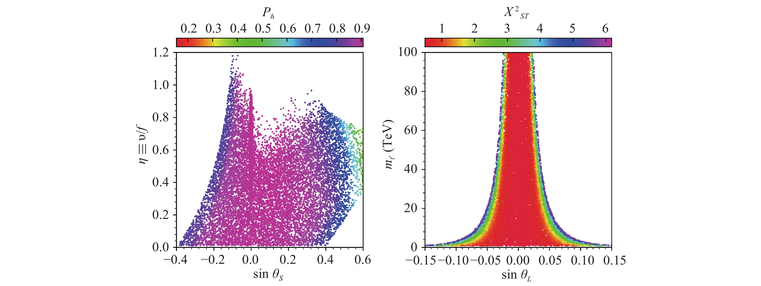
Figure 1. (color online) Selected data samples in the
${\eta \equiv v/f}$ versus${\sin\theta_S}$ (left), and${\sin\theta_L}$ versus${m_{t'}}$ (right) planes. The colors indicate${P_h}$ (left) and${\chi^2_{ST}}$ (right) , where${P_h}$ is the P value calculated with the latest LHC Run I and Run II Higgs data in HiggsSignal-2.2.0, and${\chi^2_{ST}}$ is the${\chi^2}$ in EWPD fit of the parameters${S}$ and${T}$ .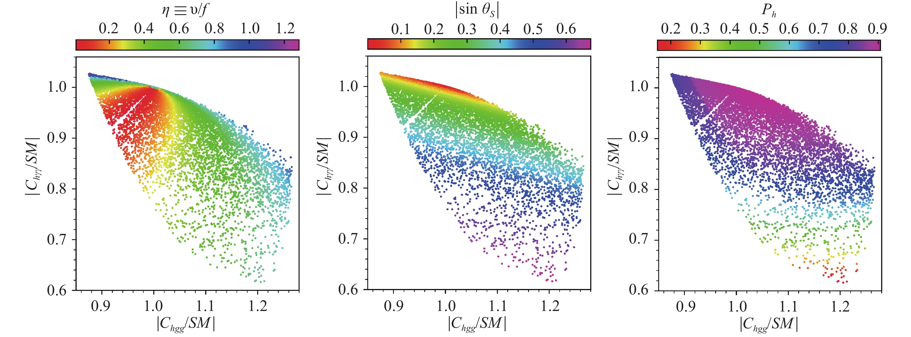
Figure 2. (color online) Identical samples as in Fig. 1, but shown in the
${|C_{h\gamma\gamma}/{\rm SM}|}$ versus${|C_{hgg}/{\rm SM}|}$ plane, which are the normalized SM-like Higgs couplings to photons and gluons, respectively. The colors indicate${\eta}$ (left),${|\sin\theta_S|}$ (middle) and${P_h}$ (right).● To fit the Higgs data over the 70% level, the normalized coupling of the SM-like Higgs to gluons and photons should satisfy
$0.8\lesssim|C_{h\gamma\gamma}/{\rm SM}|\lesssim1.05$ and$0.85\lesssim$ $|C_{hgg}/{\rm SM}|\lesssim1.25 $ .● When
$\eta\thicksim1$ , there is a negative correlation between$|C_{h\gamma\gamma}/{\rm SM}|$ and$|C_{hgg}/{\rm SM}|$ , while when$\eta\lesssim0.3$ , the two couplings are both smaller than 1.● When
$|\sin\theta_S|\lesssim0.2$ , there is also a negative correlation between$|C_{h\gamma\gamma}/{\rm SM}|$ and$|C_{hgg}/{\rm SM}|$ , the relation is roughly$C_{h\gamma\gamma}/{\rm SM} \simeq 1.27-0.27\times C_{hgg}/{\rm SM}$ , while when$|\sin\theta_S|\gtrsim0.4$ $|C_{h\gamma\gamma}/{\rm SM}|\lesssim0.9\lesssim|C_{hgg}/{\rm SM}|$ .In Fig. 3, we project the selected samples on the plane of
$\sigma^{13\rm TeV}_{\gamma\gamma}$ versus$m_{s}$ , where the colors indicate$\eta$ (left) and$|\sin\theta_S|$ (right).$\sigma^{13\rm TeV}_{\gamma\gamma}$ is the diphoton cross section of the light Higgs at the 13 TeV LHC, and the dotted and dashed curves are the exclusion limits given by ATLAS with$80$ fb-1 of data [33], and CMS with$35.9$ fb-1 of data [9], respectively. We do not use these two exclusion curves to constrain our samples, because the two results are inconsistent at 95 GeV. Instead, we use the results of the two collaborations for Run I [57, 58] as the solid constraints. On the basis of the diphoton rate of the light scalar, we can roughly sort MDM into two scenarios:● Large-diphoton scenario, which has in general a small Higgs-dilaton mixing angle (
$|\sin\theta_S|\lesssim0.2$ ) and a small dilaton VEV$f$ ($0.5\lesssim\eta\equiv v/f\lesssim1$ );● Small-diphoton scenario, which has a large Higgs-dilaton mixing angle (
$0.4\lesssim|\sin\theta_S|\lesssim0.7$ ) or a large dilaton VEV$f$ ($\eta\equiv v/f\lesssim0.3$ ).We can see that the first scenario in general predicts large diphoton rates (
$\sigma^{13\rm TeV}_{\gamma\gamma}\gtrsim 20$ fb or$\sigma^{13\rm TeV}_{\gamma\gamma}/{\rm SM}\gtrsim 0.2$ ), while the second predicts small diphoton rates ($\sigma^{13\rm TeV}_{\gamma\gamma}\lesssim 20$ fb or$\sigma^{13\rm TeV}_{\gamma\gamma}/{\rm SM}\lesssim 0.2$ ). For the central value of the excess seen by CMS at$m_{\gamma\gamma}\simeq95$ GeV,$\sigma^{13\rm TeV}_{\gamma\gamma}/{\rm SM}\simeq$ 0.64, we checked that samples with$m_s\simeq95$ GeV,$\eta\simeq0.6$ and$|\sin\theta_S|\simeq0$ fit the data well.In order to interpret the production rates of the light Higgs in the diphoton channel, we project inFig.4 the selected samples in the
$|C_{s\gamma\gamma}/{\rm SM}|$ versus$|C_{sgg}/{\rm SM}|$ plane, where the colors indicate$\eta$ (left) and$|\sin\theta_S|$ (right). The quantities$|C_{s\gamma\gamma}/{\rm SM}|$ and$|C_{sgg}/{\rm SM}|$ are the normalized light Higgs coupling to gluons and photons, respectively. From this figure we can see that:
Figure 4. (color online) Identical samples as in Fig. 1, but in the
${|C_{s\gamma\gamma}/{\rm SM}|}$ versus${|C_{sgg}/{\rm SM}|}$ plane, where the colors indicate${\eta}$ (left) and${|\sin\theta_S|}$ (right). The quantities${|C_{s\gamma\gamma}/{\rm SM}|}$ and${|C_{sgg}/{\rm SM}|}$ are the normalized light scalar couplings to photons and gluons, respectively.● For
$|\sin\theta_S|\thickapprox0$ , we checked that the ratio of the two normalized loop-induced couplings are$ \begin{align} \frac{|C_{s\gamma\gamma}/{\rm SM}|}{|C_{sgg}/{\rm SM}|} \approx 0.3, \end{align} $

(26) which can also be inferred from Eq. (13).
● Samples with small
$|\sin\theta_S|$ and large$\eta$ have large$sgg$ couplings ($0.6\lesssim|C_{sgg}/ {\rm SM}|\lesssim1.2$ ) and small$s\gamma\gamma$ couplings ($|C_{s\gamma\gamma}/ {\rm SM}|\lesssim0.3$ ). In combination with Fig. 3 , we know that these samples belong to the large-diphoton scenario.● All samples with small
$\eta$ ($\lesssim0.3$ ) have small$sgg$ and$s\gamma\gamma$ couplings ($|C_{sgg}/{\rm SM}|\lesssim0.5$ and$|C_{s\gamma\gamma}/{\rm SM}|\lesssim0.6$ ). In combination with Fig. 3 , we know that these samples belong to the small-diphoton scenario.● All samples with large
$|\sin\theta_S|$ ($\gtrsim0.4$ ) have small$sgg$ couplings ($|C_{sgg}/{\rm SM}|\lesssim0.5$ ) but large$s\gamma\gamma$ couplings ($|C_{s\gamma\gamma}/{\rm SM}|\gtrsim0.5$ ). In combination with Fig. 3 , we know that these samples also belong to the small-diphoton scenario.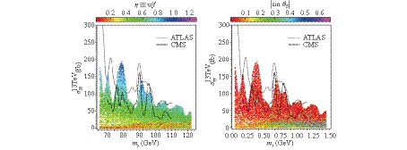
Figure 3. (color online) Identical samples as in Fig. 1, but in the
${\sigma^{13\rm TeV}_{\gamma\gamma}}$ versus${m_{s}}$ plane, where the colors indicate${\eta}$ (left) and${|\sin\theta_S|}$ (right). The curves are the exclusion limits in the search for low-mass resonance in diphoton channel at the 13 TeV LHC; dotted line: ATLAS with${80}$ fb−1 [33]; dashed line: CMS with${35.9}$ fb−1 [9] . -
In this letter, motived by the interesting topic of whether an additional scalar exists beyond the SM and our uncertainty of the physics beyond the SM in the low mass region, in particular in view of the inconsistent results of the ATLAS and CMS collaborations in their search for light resonances around 95 GeV in the diphoton channel, we study a light scalar in new physics models, which could help interpret different results in different parameter spaces, and how it could be further distinguished at the LHC. We consider the Minimal Dilaton Model, which extends the SM by a dilaton/Higgs-like singlet scalar and a vector-like top partner. In our calculations, we considered the theoretical constraints from vacuum stability and Landau pole, the experimental constraints from EWPD, the latest Higgs data from Run I and Run II of the LHC, and the low-mass Higgs/resonance searches at LEP, Tevatron and LHC. We sort the data samples obtained under these constraints into two scenarios: the large-diphoton scenario (with
$\sigma_{\gamma\gamma}/{\rm SM}\gtrsim0.2$ ) and the small-diphoton scenario (with$\sigma_{\gamma\gamma}/{\rm SM}\lesssim0.2$ ), which are favored by the CMS and ATLAS results, respectively.We compare the two scenarios, test the characteristics of the model parameters, the scalar couplings, production and decay, and consider how they could be further discerned at colliders. Finally, we draw the following conclusions:
● The large-diphoton scenario has in general a small Higgs-dilaton mixing angle (
$|\sin\theta_S|\lesssim0.2$ ) and a small dilaton VEV$f$ ($0.5\lesssim\eta\equiv v/f\lesssim1$ ), while the small-diphoton scenario has a large mixing ($|\sin\theta_S|\gtrsim0.4$ ) or a large VEV ($\eta\equiv v/f\lesssim0.3$ ).● The large-diphoton scenario in general predicts a small
$s\gamma\gamma$ coupling ($|C_{s\gamma\gamma}/{\rm SM}|\lesssim0.3$ ) and a large$sgg$ coupling ($0.6\lesssim|C_{sgg}/{\rm SM}|\lesssim1.2$ ), while the small-diphoton scenario predicts small$sgg$ coupling ($|C_{sgg}/ $ ${\rm SM}|\lesssim0.5$ ).● The large-diphoton scenario can interpret the small diphoton excess seen by CMS at its central value, when
$m_s\simeq95$ GeV,$\eta\simeq0.6$ and$|\sin\theta_S|\simeq0$ .● The large-diphoton scenario predicts a negative correlation between the Higgs couplings
$|C_{h\gamma\gamma}/{\rm SM}|$ and$|C_{hgg}/{\rm SM}|$ , while the small-diphoton scenario predicts that both couplings are smaller than 1, or$|C_{h\gamma\gamma}/{\rm SM}|\lesssim $ $0.9 \lesssim|C_{hgg}/{\rm SM}|$ .The two scenarios can also be tested via the
$s\to b\bar{b}$ channel, with$s$ produced through VBF or Vs at the LHC, and$s\to gg$ at future electron-positron colliders, where the loop effect of the top quark sector in scalar production may need to be considered. We leave this study for our future work. -
We thank Dr. Tim Stefaniak for helpful discussions on HiggsBounds and HiggsSignal.
A light scalar in the Minimal Dilaton Model in light of the LHC constraints
- Received Date: 2018-11-13
- Available Online: 2019-02-01
Abstract: Whether an additional light scalar exists is an interesting topic in particle physics beyond the Standard Model (SM), as we do not know as yet the nature of physics beyond the SM in the low mass region in view of the inconsistent results of the ATLAS and CMS collaborations in their search for light resonances around 95 GeV in the diphoton channel. We study a light scalar in the Minimal Dilaton Model (MDM). Under the theoretical and the latest experimental constraints, we sort the selected data samples into two scenarios according to the diphoton rate of the light scalar: the large-diphoton scenario (with


 DownLoad: