


 Abstract
 HTML
HTML Reference
 Related
 PDF
PDF


-
With accumulation of experimental data, more and more open-charm and open-bottom states are reported by the experiments (see the review paper [1] for more details). Among the observed states, there are abundant candidates for charmed and charmed-strange mesons including the famous
$D_{s0}(2317)$ and$D_{s1}(2460)$ . In recent years, experimentalists have especially made great progress in observing D -wave charmed mesons, as well as D -wave charmed-strange mesons. For example, the observed$D^{*}(2760)$ ,$D(2750)$ [2, 3],$D_{s1}^{*}(2860)$ and$D_{s3}^{*}(2860)$ [4, 5] are good candidates for 1D states in charmed and charmed-strange meson families [6-15]. In addition,$D_{sJ}^{*}(2860)$ [16, 17] can be assigned to a 1D state of charmed-strange meson, although there exist other interpretations [18-25]. Readers can refer to Refs. [26, 27] for more information on D -wave charmed and charmed-strange mesons.When examining the production processes involving D -wave charmed and charmed-strange mesons, we observe that these states are mainly produced via nonleptonic weak decays of bottom/bottom-strange mesons. However, as an important decay mode, semileptonic decays of
$B/B_s$ mesons are the ideal platform for producing D -wave$D/D_s$ mesons because they can be estimated more accurately than nonleptonic decays. In order to estimate the branching ratios of these processes, we need to perform a serious theoretical study of the production of D -wave$D/D_s$ mesons via the semileptonic decays of$B/B_s$ mesons, which is the main task of the present work.We adopt in this work the light-front quark model (LFQM) [28-32], which is a relativistic quark model. Since the involved light-front wave function is manifestly Lorentz invariant and the hadron spin is constructed by using the Melosh-Wigner rotation [33, 34], LFQM can be suitably applied to a study of semileptonic decays of
$B/B_s$ mesons. In Refs. [35-48], the production rates of S- and P-wave$D/D_s$ mesons have been estimated through the decay processes of$B/B_s$ in the covariant LFQM.As of yet, there has been no study of the production of D -wave
$D/D_s$ mesons via the semileptonic decays of$B/B_s$ mesons in the covariant light-front approach, which makes the present work, to our knowledge, the first paper on this issue. As shown in the following sections, the technical details relevant for the above processes are far more complicated than for S- and P-wave mesons. Thus, our work is not only an application of LFQM, but is also a development of this research field since the formulas presented can be helpful for studying other processes involving D -wave mesons. We consider this aspect valuable to the readers and provide the details of our analysis.Finally, we hope that the present study will stimulate the interest of experiments in their search for D -wave
$D/D_s$ mesons via the semileptonic decays of$B/B_s$ mesons, as it opens another window for exploring D -wave$D/D_s$ mesons and contributes to gathering more experimental information.This paper is organized as follows. In Section 2, we introduce the covariant light-front approach for D -wave mesons and their corresponding form factors. In Section 3, we give our numerical results including the form factors and the decay branching ratios. In Section 4, the relation between the light-front form factors and the requirements from the heavy quark symmetry are presented. The final section is devoted to a summary of our work. In Appendices A through E, we give the algebraic details related to the production of D -wave mesons via
$B_{(s)}$ semileptonic decay in LFQM, while Appendix F is devoted to proving the Lorentz invariance of the matrix elements in the toy model proposed in Ref. [49] with a multipole ansatz for vertex functions. -
In the conventional light-front quark model, the quark and antiquark inside a meson are required to be on their mass shells. One can then extract physical quantities by calculating the plus component of the corresponding matrix element. However, as discussed in Ref. [35], this approach may result in missing the so-called Z-diagram contribution, so that the matrix element depends on the choice of frame. A systematic way of incorporating the zero-mode effect was proposed in Ref. [49] by maintaining the associated current matrix elements frame independent, so that the physical quantities can be extracted.
In this work, we apply the covariant light-front approach to investigate the production of
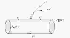
$D_{(s)}^{**}$ mesons via the semileptonic decays of$B/B_s$ mesons (see Fig. 1), where$D_{(s)}^{**}$ denotes a general D -wave$D/D_s$ meson. First, we briefly introduce how to deal with the transition amplitudes.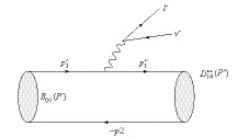
Figure 1. Diagram of the meson transition processes
${B_{(s)} \to D_{(s)}^{**}\ell^-\bar{\nu}}$ .${P^{\prime(\prime\prime)}}$ is the momentum of the incoming (outgoing) B/Bs (D-wave Ds) meson.${p_1^{\prime(\prime\prime)}}$ denotes the momentum carried by the bottom (charm) quark, while p2 is the momentum of a light quark.According to Ref. [49], the relevant form factors are calculated in terms of Feynman loop integrals, which are manifestly covariant. The constituent quarks inside a hadron are off-shell, i.e. the incoming (outgoing) meson has the momentum
$P^{\prime(\prime\prime)}=p_1^{\prime(\prime\prime)}+p_2$ , where$p_1^{\prime(\prime\prime)}$ and$p_2$ are the off-shell momenta of the quark and antiquark, respectively. These momenta can be expressed in terms of the appropriate internal variables$(x_i, p_{\bot}^{\prime})$ , defined by,$ p_{1}^{\prime+}=x_{1}P^{\prime+}, \quad\quad\quad p^+_2 = x_2P^{\prime+}, $

(1) $ p_{1\bot}^{\prime}=x_{1}P^{\prime}_{\bot}+ p^{\prime}_{\bot}, \quad p_{2\bot}=x_{2}P^{\prime}_{\bot}- p^{\prime}_{\bot}, $

(2) with
$x_1+x_2=1$ . In the light-front coordinates,$P^{\prime}=(P^{\prime-}, $ $P^{\prime+}, P_{\bot}^{\prime}) $ with$P^{\prime\pm}=P^{\prime0}\pm P^{\prime3}$ , which satisfy the relation$P^{\prime2}=P^{\prime+}P^{\prime-}-P^{\prime2}_{\bot}$ . One needs to point out that there exist different conventions for momentum conservation in the covariant light-front and conventional light-front approaches. In the covariant light-front approach, four components of a momentum are conserved at each vertex, where the quark and antiquark are off-shell. In the conventional light-front approach, the plus and transverse components of a momentum are conserved quantities, where the quark and antiquark are required to be on their mass shells. Thus, it is useful to define internal quantities for on-shell quarks$ M_0^{\prime2}=(e_1^{\prime}+e_2)^2=\frac{p_{\bot}^{\prime2}+m_1^{\prime2}}{x_1} +\frac{p_{\bot}^{\prime2}+m_2^{2}}{x_2}, $

(3) $ \tilde{M}_{0}^{\prime}=\sqrt{M_{0}^{\prime2}-(m_1^{\prime}-m_2)^2}, $

(4) $ e_{1}^{\prime}=\sqrt{m_1^{\prime2}+p_{\bot}^{\prime2}+p_z^{\prime2}}, \quad e_{2}=\sqrt{m_2^{2}+p_{\bot}^{\prime2}+p_z^{\prime2}}, $

(5) $ p_z^{\prime}=\frac{x_2 M_0^{\prime}}{2}-\frac{m_2^2+p_{\bot}^{\prime2}}{2x_2M_0^{\prime}}, $

(6) where
$M_0^{\prime2}$ is the kinetic invariant mass squared of the incoming meson.$e^{(\prime)}_i$ denotes the energy of quark$i$ , while$m_1^{\prime}$ and$m_2$ are the masses of the quark and antiquark, respectively.In Ref. [35], the form factors for semileptonic decays of bottom mesons into S -wave and P -wave charmed mesons were obtained within the framework of the covariant light-front quark model. In the following, we adopt the same approach to deduce the form factors for the production of D -wave charmed/charmed-strange mesons by semileptonic decays of bottom/bottom-strange mesons. Here, D -wave
$D/D_s$ mesons, denoted as$D^{*}_{(s)1}$ ,$D^{*}_{(s)2}$ ,$D^{*\prime}_{(s)2}$ , and$D^{*}_{(s)3}$ , have quantum numbers${}^{2S+1}L_J={}^3D_1, {}^1D_2, {}^3D_2, $ and${}^3D_3$ , respectively. In the following, we use this notation for simplicity.In the heavy quark limit
$m_Q\rightarrow \infty$ , the heavy quark spin$s_Q$ decouples from the other degrees of freedom. Hence, a more convenient way to describe charmed/charmed-strange mesons is to use the$|J, j_{\ell}\rangle$ basis, where$J$ denotes the total spin and$j_\ell$ denotes the total angular momentum of the light quark. There exists a connection between the physical states$|J, j_{l}\rangle$ and the states described by$|J, S\rangle$ for$L=2$ [50, 51], i.e.,$ |D_{(s){5\over2}} \rangle\equiv\left|2, {5\over2}\right\rangle=\sqrt{\frac{3}{5}}\left|D^{*}_{(s)2}\right\rangle+\sqrt{\frac{2}{5}}\left|D^{*\prime}_{(s)2}\right\rangle, $

(7) $ |D'_{(s){3\over2}}\rangle\equiv\left|2, {3\over2}\right\rangle=-\sqrt{\frac{2}{5}}\left|D^{*}_{(s)2}\right\rangle+\sqrt{\frac{3}{5}}\left|D^{*\prime}_{(s)2}\right\rangle. $

(8) This relation shows that two physical states
$D_{(s)2}$ and$D_{(s)2}^{\prime}$ with$J^P=2^-$ are linear combinations of$D^{*}_{(s)2}({}^1D_2)$ and$D^{*\prime}_{(s)2}({}^3D_2)$ states. When dealing with the transition amplitudes for the production of$D_{(s)2}$ and$D_{(s)2}^{\prime}$ states, we need to consider the mixing of states as in Eqs. (7) and (8).One can write the general definition of the matrix elements for the production of D -wave
$D/D_s$ mesons via the semileptonic decays of$B/B_s$ mesons, i.e.,$ \begin{split} & \left\langle D^{*}_{(s)1}(P'', \epsilon'')\left|V_{\mu}\right|B_{(s)}(P^\prime)\right\rangle=\epsilon_{\mu\nu\alpha\beta}\epsilon''^{*\nu}P^{\alpha}q^{\beta}g_D(q^{2}), \\ &\left\langle D^{*}_{(s)1}(P'', \epsilon'')\left|A_{\mu}\right |B_{(s)}(P^\prime)\right\rangle=\\ &\quad-i\left\{\epsilon''^{*}_{\mu}f_D(q^2)+\epsilon''^{*}\cdot P\left[P_{\mu} a_{D+}(q^2)+q_{\mu}a_{D-}(q^2)\right]\right\}, \end{split} $

(9) $ \begin{split} &\left\langle D^{*}_{(s)2}(P'', \epsilon'')\left|A_{\mu}\right|B_{(s)}(P')\right\rangle=-\epsilon_{\mu\nu\alpha\beta}\epsilon''^{*\nu\lambda}P_{\lambda}P^{\alpha}q^{\beta}n(q^2), \\ &\left\langle D^{*}_{(s)2}(P'', \epsilon'')\left|V_{\mu}\right|B_{(s)}(P')\right\rangle=\\ &\quad i\left\{m(q^2)\epsilon''^{*}_{\mu\nu}P^{\nu}+\epsilon''^{*}_{\alpha\beta}P^{\alpha}P^{\beta} \left[P_{\mu}z_{+}(q^2)+ q_{\mu}z_{-}(q^2)\right]\right\}, \end{split}$

(10) $ \begin{split} &\left\langle D^{*\prime}_{(s)2}(P'', \epsilon'')\left|A_{\mu}\right|B_{(s)}(P')\right\rangle=-\epsilon_{\mu\nu\alpha\beta}\epsilon''^{*\nu\lambda}P_{\lambda}P^{\alpha}q^{\beta}n'(q^2), \\ &\left\langle D^{*\prime}_{(s)2}(P'', \epsilon'')\left|V_{\mu}\right|B_{(s)}(P')\right\rangle =\\ &\quad i\left\{m'(q^2)\epsilon''^{*}_{\mu\nu}P^{\nu}+\epsilon''^{*}_{\alpha\beta}P^{\alpha}P^{\beta}\left[P_{\mu}z'_{+}(q^2)+ q_{\mu}z'_{-}(q^2)\right]\right\}, \end{split}$

(11) $\begin{split} &\left\langle D^{*}_{(s)3}(P'', \epsilon'')\left|V_{\mu}\right|B_{(s)}(P')\right\rangle=\epsilon_{\mu\nu\alpha\beta}\epsilon''^{*\nu\lambda\sigma}P_{\lambda}P_{\sigma}P^{\alpha}q^{\beta}y(q^2), \\ &\left\langle D^{*}_{(s)3}(P'', \epsilon'')\left|A_{\mu}\right|B_{(s)}(P')\right\rangle=\\ &\quad -i\left\{w(q^2)\epsilon''^{*}_{\mu\nu\alpha}P^{\nu}P^{\alpha}+\epsilon''^*_{\alpha\beta\gamma}P^{\alpha}P^{\beta}P^{\gamma} \left[P_{\mu}o_{+}(q^2)+q_{\mu}o_{-}(q^2)\right]\right\}. \end{split}$

(12) Here,
$P=P^{\prime}+P^{\prime\prime}$ ,$q=P^{\prime}-P^{\prime\prime}$ and$\epsilon_{0123}=1$ .$\epsilon^{\prime*}_{\mu}$ ,$\epsilon^{\prime\prime*}_{\mu\nu}$ and$\epsilon^{\prime\prime*}_{\mu\nu\alpha}$ are the polarization vector (tensors). The details of the derivation are given in Appendix E. The Lorentz invariance has been assumed when deriving these form factors. One should note that the$B_{(s)}\rightarrow D_{(s)}^{**}$ transition occurs through a$V-A$ current, where$D_{(s)}^{**}$ denotes the general$D$ -wave charmed (charmed-strange) meson. For the semileptonic decays involving${}^3D_1$ and${}^3D_3$ states, a$\epsilon_{\mu\nu\alpha\beta}$ term arises in$\left\langle D^{*}_{(s)1}\left(D^{*}_{(s)3}\right)\left|V_{\mu}\right|B_{(s)}\right\rangle$ , which corresponds to the contribution of the vector current. Contrary to the case of${}^3D_1$ and${}^3D_3$ states, for${}^1D_2$ and${}^3D_2$ states, the$\epsilon_{\mu\nu\alpha\beta}$ term arises from the axial vector current. A minus sign is added in front of this term, so that we have$\left\langle D_{(s)2}^{*(\prime)}\left|-A_\mu\right|B_{(s)}\right\rangle=\epsilon_{\mu\nu\alpha\beta}\epsilon ^{\prime\prime*\nu\lambda}P_{\lambda}P^{\alpha}q^{\beta}n^{(\prime)}(q^2)$ . When the sign of the$\epsilon_{\mu\nu\alpha\beta}$ term is fixed, the signs of the other form factors can also be determined.We now focus on the hadronic matrix elements given by Eqs. (9)-(12). Here, we show how to calculate them by taking the
$B_{(s)}\rightarrow D_{(s)1}^{*}$ transition as an example, where$D_{(s)1}^{*}$ denotes the${}^3D_1$ state of the charmed/charmed-strange meson. The corresponding matrix element for$B_{(s)}\rightarrow D_{(s)1}^{*}$ can be written as$ B_{\mu}^{B_{(s)}(D^{*}_{(s)1})}\equiv\left\langle D_{(s)1}^{*}(P^{\prime\prime}, \epsilon^{\prime\prime*})\left|V_{\mu}-A_{\mu}\right|B_{(s)}(P^{\prime})\right\rangle, $

(13) Following the calculations in Ref. [35], we first obtain the
$B_{(s)}\rightarrow D^{*}_{(s)1}$ transition form factors, and then calculate the processes involving the other D -wave charmed/charmed-strange states. The details for the other matrix elements are given in Appendix A. Here, one needs to introduce the vertex wave functions to describe$B_{(s)}$ and$D_{(s)1}^{*}$ mesons. The expression for a vertex function for an initial$B_{(s)}$ meson was obtained in Ref. [35]. In the following, we give a detailed discussion for the vertex function of the final state$D_{(s)1}^{*}$ meson.The D -wave vertex function has been studied in Ref. [52]. We list all D -wave vertex functions in Appendix B; one may refer to Ref. [52] for more details. First, we use
${}^3D_1$ vertex functions for calculating the$B_{(s)}\rightarrow D_{(s)1}^{*}$ transition.In the conventional LFQM,
$p'_1$ and$p_2$ are on their mass shell, while in the covariant [49] light-front approach, the quark and antiquark are off-shell, but the total momentum$P'=p'_1+p_2$ is still the on-shell momentum of a meson, i.e.$P^{\prime 2}=M^{\prime 2}$ , where$M'$ is the mass of the incoming meson. One needs to relate the vertex function deduced in the conventional LFQM to the vertex in the covariant light-front approach. A practical method for this process has been proposed in a covariant light-front approach in Ref. [49]. We obtain the corresponding covariant vertex function as$ iH_{{}^3D_1}\left[\gamma_{\mu}-\frac{1}{W_{{}^3D_1}}\left(p^\prime_1-p_2\right)_{\mu}\right]\epsilon^{\mu}, $

(14) where
$H_{{}^{3}D_1}$ and$W_{{}^{3}D_1}$ denote the corresponding scalar functions for${}^3D_1$ state.The explicit expression for the matrix element
$B_{\mu}^{B_{(s)}D^{*}_{(s)1}}$ , which corresponds to the hadronic one-loop Feynman diagram of Fig. 2, reads
Figure 2. (color online) A hadronic one-loop Feynman diagram for the process shown in Fig. 1. The V-A current is attached to a blob in the upper middle of the circle.
$ B_{\mu}^{B_{(s)}D^{*}_{(s)1}}=-i^3\frac{N_c}{(2\pi)^4}\int {\rm d}^4p^{\prime}_1\frac{H^{\prime}_{P}\left(iH^{\prime\prime}_{{}^3D_1}\right)}{N_1^{\prime}N_1^{\prime\prime}N_2}S_{\mu\nu}^{{}^3D_1}\epsilon^{*\prime\prime\nu}, $

(15) where
$N_c$ is the number of colors,$N_1^{\prime(\prime\prime)}=p_1^{\prime(\prime\prime)2}-m_1^{\prime(\prime\prime)2}+i\epsilon$ ,$N_2=p_2^{2}-m_2^{2}+i\epsilon$ .$H^{\prime}_{P}\gamma_5$ is the vertex function of a pseudoscalar meson, and$ \begin{split} S^{^{3D_1}}_{\mu\nu}=&{{\rm Tr}\Bigg\{\left[\gamma_{\nu}-\frac{1}{W^{\prime\prime}_{{}^3D_1}}\left(p^{\prime\prime}_1-p_2\right)_{\nu}\right]} \left({\not \!\!{p}}^{\prime\prime}_{1}+m^{\prime\prime}_1\right)\gamma_{\mu}\left(1-\gamma_5\right)\\ &\left({\not \!\!{p}}^{\prime}_1+m^{\prime}_1\right)\gamma_5\left(-{\not \!\!{p}}_2+m_2\right)\Bigg\}. \end{split} $

(16) One can integrate over
$p_1^{\prime-}$ via a contour integration with${\rm d}^4p^{\prime}_1=P^{~\prime +}{\rm d}p^{\prime -}_1 {\rm d}x_2{\rm d}^2p^\prime_\bot/2$ and the integration picks up a residue$p_2=\hat{p}_2$ , where the antiquark is set to be on-shell,$\hat{p}_2^2=m_2^2$ . The momentum of the quark is given by the momentum conservation,$\hat{p}_1^{\prime}=P^{\prime}-\hat{p}_2$ . Consequently, after performing the$p_1^{\prime-}$ integration, we make the replacements:$ \begin{aligned} N_1^{\prime(\prime\prime)}&\rightarrow \hat{N}_1^{\prime(\prime\prime)}=x_1\left(M^{\prime(\prime\prime)2}-M_0^{\prime(\prime\prime)2}\right), \\ H^{\prime}_P&\rightarrow h_{P}^{\prime}, \\ H^{\prime\prime}_{{}^3D_1}&\rightarrow h^{\prime\prime}_{{}^3D_1}, \\ W^{\prime\prime}_{{}^3D_1}&\rightarrow \omega^{\prime\prime}_{{}^3D_1}, \\ \int \frac{{\rm d}^4p_1^{\prime}}{N_1^{\prime}N_1^{\prime\prime}N_2}H^{\prime}_P H^{\prime\prime}_{{}^3D_1}S^{{}^3D_1}_{\mu\nu}&\rightarrow -i\pi\int \frac{{\rm d}x_2{\rm d}^2p_{\bot}^{\prime}}{x_2\hat{N}_1^{\prime}\hat{N}_1^{\prime\prime}} h^{\prime}_Ph^{\prime\prime}_{{}^3D_1}\hat{S}^{{}^3D_1}_{\mu\nu}, \end{aligned} $

where the explicit trace expansion of
$\hat{S}_{\mu\nu}^{{}^3D_1}$ , after integrating Eq. (15) over$p_1^{\prime-}$ , is presented in Appendix A. In addition,$h^{\prime}_P$ is given in Ref. [35] as,$ h_{P}^{\prime}=\left(M^{\prime2}-M_{0}^{\prime2}\right)\sqrt{\frac{x_1x_2}{N_c}} \frac{1}{\sqrt{2}\tilde{M}_0^{\prime}}\varphi, $

(17) where
$\varphi$ is the solid harmonic oscillator for$S$ -wave and describes the momentum distribution of the initial$B_{(s)}$ meson.As noted in Ref. [52], after carrying out the contour integral over
$p_1^{\prime-}$ , the quantities$H^{\prime\prime}_{{}^3D_1}$ ,$W^{\prime\prime}_{{}^3D_1}$ and$\epsilon^{*\prime\prime}$ are replaced by$h^{\prime\prime}_{{}^3D_1}$ ,$\omega^{\prime\prime}_{{}^3D_1}$ and$\hat{\epsilon}^{*\prime\prime}$ , respectively. Here,$h_{{}^3D_1}^{\prime\prime}$ is related to$h_{{}^3D_1}^{\prime}$ as,$ h^{\prime\prime}_{{}^3D_1}=\left(M^{\prime\prime2}-M_0^{\prime\prime2}\right)\sqrt{x_1x_2}h^{\prime}_{{}^3D_1}, $

(18) which is derived in Appendix B, and
$ M_0^{\prime\prime2}=\frac{p^{\prime2}_{\bot}+m_1^{\prime\prime2}}{x_1}+ \frac{p^{\prime\prime2}_{\bot}+m_2^2}{x_2}, $

(19) with
$p^{\prime\prime}_{\bot}=p^{\prime}_{\bot}-x_2q_{\bot}$ .As pointed out in Refs. [35, 49],
$\hat{p}_1^{\prime}$ can be expressed in terms of the external vectors,$P^{\prime}$ and$\tilde{\omega}$ :$\begin{aligned} {\hat p^{\prime \mu }}_1 =& {\left( {{P^\prime } - {{\hat p}_2}} \right)^\mu } = {x_1}{P^{\prime \mu }} + {(0,0,p_ \bot ^\prime )^\mu } \\ &+ \frac{1}{2}\left( {{x_2}{P^{\prime - }} - \frac{{p_{2 \bot }^2 + m_2^2}}{{{x_2}{P^{\prime + }}}}} \right){\tilde \omega ^\mu }, \end{aligned} $

where
$\tilde{\omega}=(\tilde\omega^+, \tilde\omega^-, \tilde\omega_\bot)=(2, 0, 0_{\bot})$ [35, 49] is a light-like four vector in the light-front coordinate system. Since the constant vector$\tilde{\omega}$ is not Lorentz covariant, the presence of$\tilde\omega$ terms implies that the corresponding matrix elements are not Lorentz invariant. This$\tilde{\omega}$ dependence also appears in the products of two$\hat{p}_1^{\prime}$ 's. This spurious contribution is related to the so-call zero-mode effect and should be canceled when calculating physical quantities.Initiated by the toy model proposed in Ref. [49], Jaus developed a method which allows calculating the zero-mode contributions associated with the corresponding matrix element.
$\hat{p}_1^{\prime}$ as well as the products of a couple of$\hat{p}_1^{\prime}$ 's can be decomposed into products of vectors$P$ ,$q$ ,$\tilde\omega$ , and$g_{\mu\nu}$ , as shown in Appendix C, with functions$A^{(m)}_n$ ,$B^{(m)}_n$ , and$C^{(m)}_n$ , where$B^{(m)}_n$ and$C^{(m)}_n$ are related to$\tilde{\omega}$ -dependent terms. Based on the toy model, the vertex function of a ground state pseudoscalar meson is described by a multipole ansatz,$ H_0(p_1^2, p_2^2)=\frac{g}{N^n_{\Lambda}}, $

(20) which is different from our conventional vertex functions. Jaus has proven that at the toy model level, the spurious loop integrals of
$B^{(2)}_{1}$ ,$B_{1, 2}^{(3)}$ and$C^{(2)}_{1}$ ,$C_{1, 2}^{(3)}$ vanish in the following integrals,$ \frac{i}{(2\pi)^4}\int {\rm d}^4p^\prime_1\frac{M^{(m)}_n}{N^\prime_\Lambda N_1^{\prime}N_2N_1^{\prime\prime}N^{\prime\prime}_\Lambda}, $

(21) where
$M^{(m)}_n\equiv B^{(m)}_{n}$ or$C^{(m)}_n$ . This fact is a natural consequence of the Lorentz invariance of the theory. The$\tilde{\omega}$ -dependent terms have been systematically eliminated in the toy model since the$B^{(2)}_{1}$ and$C^{(2)}_{1, 2}$ give trivial contributions to the calculated form factors [49].However, this method has a narrow scope of application. Note that Jaus proposed this method in a very simple multipole ansatz for the vertex function. One may get totally different contributions from the zero-mode effects once the form of a vertex function for a meson is changed. For instance, as indicated in Ref. [53], for the weak transition form factors between pseudoscalar and vector meson, the zero-mode contributions depend on the form of the vector meson vertex,
$ \Gamma^{\mu}=\gamma^{\mu}-(2k-P_V)^{\mu}/D, $

(22) where the denominator
$D$ contains different types of terms. (Readers can also refer to Refs. [54-59] for more details.)Beyond the toy model, the method of including the zero-mode contributions in Ref. [49] was further applied to study the decay constants and form-factors for
$S$ -wave and$P$ -wave mesons [35]. In Ref. [35], Cheng et al. used the vertex functions for S- and P-wave mesons deduced from the conventional light-front quark model, which are different from the multipole ansatz proposed by Jaus. In [35] , they applied the method of the toy model to cancel the$C^{(m)}_{n}$ functions. As for$B^{(m)}_n$ functions, they have numerically checked that$B^{(m)}_n$ give very small contributions to the corresponding form factors. That is, when the multipole vertices are replaced by conventional light-front vertex functions, and by setting$B_n^{(m)}$ and$C^{(m)}_{n}$ functions equal to 0, one can still obtain very good numerical results for the decay constants. Indeed, as indicated in Ref. [49], the numerical results obtained by applying conventional vertices are even better than those for vertices from the multipole ansatz.It is natural to expect that this method can also be applied in our calculations of the form factors for the transition processes of D -wave mesons. In order to calculate the corresponding form factors, one also needs to eliminate the
$B^{(m)}_n$ and$C^{(m)}_n$ functions introduced in the D -wave transition matrix elements. In the following, we introduce our analysis of the zero-mode contributions.Following the discussion in Refs. [35, 49], to avoid the
$\tilde{\omega}$ dependence of$\hat{p}_{1}^{\prime}$ , as well as of the product of a couple of$\hat{p}^{\prime}_{1}$ 's, one needs to do the following replacements:$ \hat{p}_{1\mu}^{\prime}\doteq P_{\mu}A_1^{(1)}+q_{\mu}A_2^{(1)}, $

(23) $ \begin{split} \hat{p}_{1\mu}^{\prime}\hat{p}_{1\nu}^{\prime}\doteq & g_{\mu\nu}A_1^{(2)}+P_{\mu}P_{\nu}A_2^{(2)}+\left(P_{\mu}q_{\nu}+q_{\mu}P_{\nu}\right) A_3^{(2)} \\ &+q_{\mu}q_{\nu}A_4^{(2)}, \end{split} $

(24) $ \begin{split} \hat{p}^{\prime}_{1\mu}\hat{p}^{\prime}_{1\nu}\hat{p}^{\prime}_{1\alpha}\doteq&\left(g_{\mu\nu}P_{\alpha}+g_{\mu\alpha}P_{\nu}+g_{\nu\alpha}P_{\mu}\right)A_1^{(3)}\\ & +\left(g_{\mu\nu}q_{\alpha}+g_{\mu\alpha}q_{\nu}+g_{\nu\alpha}q_{\mu}\right) A_2^{(3)} \\&+P_{\mu}P_{\nu}P_{\alpha}A_3^{(3)}+\left(P_{\mu}P_{\nu}q_{\alpha}+P_{\mu}q_{\nu}P_{\alpha} \right.\\&\left.+q_{\mu}P_{\nu}P_{\alpha}\right)A_4^{(3)} +\left(q_{\mu}q_{\nu}P_{\alpha}+q_{\mu}P_{\nu}q_{\alpha}\right.\\&\left.+P_{\mu}q_{\nu}q_{\alpha}\right) A_5^{(3)}+q_{\mu}q_{\nu}q_{\alpha}A_6^{(3)}, \end{split} $

(25) where the
$B_n^{(m)}$ and$C^{(m)}_{n}$ functions are disregarded at the toy model level, and their loop integrals vanish manifestly if conventional vertices are introduced. We give more details in the following discussion.For the terms of products that are associated with
$\hat{N}_2$ , the zero-mode contributions are introduced and the following replacements should be made to eliminate the$\tilde{\omega}$ -dependent terms$ \begin{split} \hat{N}_2\rightarrow Z_2 =&\hat N'_1+m_1^{\prime 2}-m_2^2+(1-2x)M^{\prime 2} \\ &+\left[q^2+(qP)\right]\frac{p_\perp^\prime q_\perp}{q^2}, \end{split} $

(26) $ \hat{p}_{1\mu}^{\prime}\hat{N}_2\rightarrow P_{\mu}(A_1^{(1)}Z_2-A_1^{(2)})+q_{\mu}\left[A_2^{(1)}Z_2+\frac{q\cdot P}{q^2}A_1^{(2)}\right], $

(27) $ \begin{split} \hat{p}_{1\mu}^{\prime}\hat{p}_{1\nu}^{\prime}\hat{N}_2\rightarrow&g_{\mu\nu}A_1^{(2)}Z_2+P_{\mu}P_{\nu}(A_2^{(2)}Z_2-2A_1^{(3)})\\&+(P_{\mu}q_{\nu}+q_{\mu}P_{\nu})(A_3^{(2)}Z_2+A_1^{(3)}\frac{q\cdot P}{q^2}-A_2^{(3)})\\&+q_{\mu}q_{\nu}\Big[A_4^{(2)}Z_2+2\frac{q\cdot P}{q^2}A_2^{(1)}A_1^{(2)}\Big], \end{split} $

(28) where
$P=P^\prime+P^{\prime\prime}$ and$A_j^{(i)}$ and$Z_2$ are functions of$x_1$ ,$p^{\prime 2}_{\bot}$ ,$p^{\prime}_{\bot}\cdot q_{\bot}$ , and$q^2$ . These functions have been obtained in Ref. [49]. Again, in the above replacements,$B_n^{(m)}$ and$C^{(m)}_{n}$ can be naturally disregarded at the toy model level and their loop integrals vanish manifestly with a standard meson vertex.Let us take the second rank tensor decomposition
$\hat{p}^{\prime}_{1\mu}\hat{p}^{\prime}_{1\nu}$ as an example how to effectively set the$B_n^{(m)}$ and$C^{(m)}_{n}$ functions to 0 and eliminate the$\tilde{\omega}$ -dependent terms. There are two$\tilde{\omega}$ -dependent functions in the leading order of$\tilde{\omega}$ -decomposition, i.e.$B_1^{(2)}$ and$C_1^{(2)}$ .From Ref. [49] we have
$ B_{1}^{(2)} = A_1^{(1)}C_1^{(1)}-A_1^{(2)}, $

(29) By introducing the explicit expression of
$C_1^{(1)}$ from Ref. [49], one can easily obtain$ B_1^{(2)} = -A_1^{(1)}N_2+A_1^{(1)}Z_2-A_1^{(2)} $

(30) in the toy model. The loop integral of
$B_1^{(2)}$ naturally vanishes. On the other hand, beyond the toy model, this term should also be eliminated manifestly, i.e. we have the replacement$ A_1^{(1)}\hat{N}_2\rightarrow A_1^{(1)}Z_2-A_1^{(2)}. $

(31) The same procedure can be applied to
$C_{1}^{(2)}$ , which gives,$ A_2^{(1)}\hat{N}_2\rightarrow A_2^{(1)}Z_2+\frac{q\cdot P}{q^2}A_1^{(2)}. $

(32) We would like to emphasize that beyond the toy model, when the conventional light-front vertex functions are introduced, elimination of
$B_n^{(m)}$ is also necessary when calculating semileptonic form factors with$S$ -wave and$P$ -wave mesons as final states. However, one would obtain very small corrections since, as described earlier, these$B_n^{(m)}$ functions give small contributions.Expanding
$\hat{S}_{\mu\nu}^{{}^3D_1}$ , and replacing the$\hat{p}^{\prime}_{1\mu}\hat{p}^{\prime}_{1\nu}\hat{N}_2$ ,$\hat{p}^{\prime}_{1\mu}\hat{p}^{\prime}_{1\nu}$ ,$\hat{p}^{\prime}_{1\mu}\hat{N}_2$ ,$\hat{p}^{\prime}_{1\mu}$ , and$\hat{N}_2$ terms with the replacements in Eqs. (23)-(24) and Eqs. (26)-(28), we can obtain the form factors for the${}^3D_{1}$ state by comparing with the general definition of a matrix element given in Eq. (9). We note that, since in the expansion of$\hat{S}_{\mu\nu}^{{}^3D_1}$ there is no term with three$\hat{p}_1^{\prime}$ 's, Eq. (25) is not used. This equation just helps to find the tensor decomposition of$\hat{p}^{\prime}_{1\mu}\hat{p}^{\prime}_{1\nu}\hat{N}_2$ . This procedure is identical to what was used for the tensor decomposition of$\hat{p}^{\prime}_{1\mu}\hat{N}_2$ by analyzing the product of$\hat{p}^{\prime}_{1\mu}\hat{p}^{\prime}_{1\nu}$ .After including the zero-mode effect introduced by the
$B_n^{(m)}$ and$C^{(m)}_{n}$ functions, we get the explicit form factors$g_D(q^2)$ ,$f_{D}(q^2)$ ,$a_{D+}(q^2)$ and$a_{D-}(q^2)$ as$ g_{D}(q^2)=-\frac{N_c}{16\pi^3}\int {\rm d}x_2 {\rm d}^2 p^\prime_\bot \frac{2 h^\prime_P h^{\prime\prime}_{{}^3D_1}}{\left(1-x\right)\hat{N}^\prime_1 \hat{N}^{\prime\prime}_1}\left\{\left[A_1^{(1)}\left(2m_2-m_1^{\prime\prime}-m_1^{\prime}\right)+A_2^{(1)} \left(m_1^{\prime\prime}-m_1^\prime\right)+m_1^\prime\right]-\frac{2}{\omega^{\prime\prime}_{{}^3D_1}}A_1^{(2)}\right\}, $

(33) $ \begin{split} f_{D}(q^2)=&\frac{N_{c}}{16\pi^3}\int {\rm d}x_2 {\rm d}^2 p^\prime_\bot \frac{2 h^\prime_{P} h^{\prime\prime}_{{}^3D_1}}{\left(1-x\right)\hat{N}^\prime_1\hat{N}^{\prime\prime}_1} \Bigg\{2\bigg[4A_1^{(2)}\left(m_2-m^{\prime}_i\right)+m_2^2\left(m^{\prime\prime}_1+m^{\prime}_1\right)- m_2\Big[\left(m_1^{\prime\prime}+m_1^{\prime}\right)^2+x\left(M^{\prime\prime2}-M_0^{\prime\prime2}\right)\\&+ x\left(M^{\prime2}-M_0^{\prime2}\right)-q^2\Big]+m_1^{\prime\prime}\left[m_1^{\prime}m_1^{\prime\prime} +m_1^{\prime2}-M^{\prime2}+x\left(M^{\prime2}-M_0^{\prime2}\right)+Z_2\right]+m_1^{\prime} \left[-M^{\prime\prime2}+x\left(M^{\prime\prime2}-M_0^{\prime\prime2}\right)+Z_2\right]\bigg]\\&+4\frac{A_1^{(2)}}{\omega^{\prime\prime}_{{}^3D_1}}\left[2m_2\left(-m_2-m_1^{\prime\prime}+m_1^{\prime}\right) +2m_1^{\prime\prime}m_1^{\prime}+M^{\prime\prime2}+ M^{\prime2}-q^2-2Z_2\right] \Bigg\}, \end{split}$

(34) $ \begin{split} a_{D+}(q^2)= &\frac{N_c}{16\pi^3}\int {\rm d}x_2 {\rm d}^2 p^{\prime}_{\bot}\frac{h^{\prime}_{P}h^{\prime\prime}_{{}^3D_1}}{\left(1-x\right)\hat{N}^\prime_1\hat{N}^{\prime\prime}_1}\Bigg\{ -2\left[A_1^{(1)}\left(2m_2+m_1^{\prime\prime}-5m_1^{\prime}\right)+m_1^{\prime}\right]-2A_2^{(1)}\left(-m_1^{\prime\prime}-m_1^{\prime}\right)- 2\left(A_2^{(2)}+A_3^{(2)}\right)\left(4m_1^{\prime}-4m_2\right)\\&+ \frac{2}{\omega^{\prime\prime}_{{}^3D_1}}\bigg[\left(A_1^{(1)}-A_2^{(2)}-A_3^{(2)}\right)\left(4m_2^2+4m_2m^{\prime\prime}_1 -4m_2m_1^{\prime}-4m_1^{\prime\prime}m_1^{\prime}-2M^{\prime\prime2}-2M^{\prime2}+2q^2\right)+ \left(-A_1^{(1)}-A_2^{(1)}+1\right)\\&\times\left[m_1^{\prime\prime2}+2m_1^{\prime\prime}m_1^{\prime}+m_1^{\prime2} +x\left(M^{\prime\prime2}-M_0^{\prime\prime2}\right)+x\left(M^{\prime2}-M_0^{\prime2}\right)-q^2\right]+4\Bigg(A_1^{(1)}Z_2-A_1^{(2)}- \left(A_2^{(2)}Z_2-2A_1^{(1)}A_1^{(2)}\right)\\& -\left(A_1^{(1)}A_2^{(1)}Z_2+A_1^{(1)}A_1^{(2)}\frac{m_B^2-m_D^2}{q^2}-A_1^{(2)}A_2^{(1)}\right)\Bigg)\bigg]\Bigg\}, \end{split} $

(35) $\begin{split} a_{D-}(q^2)=&\frac{N_c}{16\pi^3}\int {\rm d}x_2 {\rm d}^2 p^{\prime}_{\bot}\frac{h^{\prime}_{P}h^{\prime\prime}_{{}^3D_1}}{\left(1-x\right)\hat{N}^\prime_1\hat{N}^{\prime\prime}_1}\Bigg\{ -2A_1^{(1)}\left(2m_2-m_1^{\prime\prime}-3m_1^{\prime}\right)-2A_2^{(1)}\left(4m_2+m_1^{\prime\prime} -7m_1^{\prime}\right)-\left(2A_3^{(2)}+2A_4^{(2)}\right)\left(4m_1^{\prime}-4m_2\right)\\&-6m_1^{\prime}+ \frac{1}{\omega^{\prime\prime}_{{}^3D_1}}\bigg[\left(2A_1^{(1)}+2A_2^{(1)}-2\right)\Big[2m_2^2-4m_2m_1^{\prime}-m_1^{\prime\prime2} -2m_1^{\prime\prime}m_1^{\prime}+m_1^{\prime2}-2M^{\prime2}- x\left(M^{\prime\prime2}-M_0^{\prime\prime2}\right)\\&+x\left(M^{\prime2}-M_0^{\prime2}\right)+q^2\Big]+ \left(2A_3^{(2)}+2A_4^{(2)}-2A_2^{(1)}\right)\left(-4m_2^2-4m_2m_1^{\prime\prime}+4m_2m_1^{\prime} +4m_1^{\prime\prime}m_1^{\prime}+2M^{\prime\prime2}+2M^{\prime2}-2q^2\right)\\&+12\left(A_2^{(1)}Z_2+ \frac{M^{\prime2}-M^{\prime\prime2}}{q^2}A_1^{(2)}\right)- 8\left(A_4^{(2)}Z_2+2\frac{M^{\prime2}-M^{\prime\prime2}}{q^2}A_2^{(1)}A_1^{(2)}\right)-4Z_2+4\Bigg(A_1^{(1)}Z_2 -A_1^{(2)}-2\Big(A_1^{(1)}A_2^{(1)}Z_2\\&+A_1^{(1)}A_1^{(2)}\frac{m_B^2-m_D^2}{q^2}-A_1^{(2)}A_2^{(1)}\Big)\Bigg) \bigg]\Bigg\}.\end{split} $

(36) The same procedure can also be applied for the transitions in the case of
${}^1D_2$ ,${}^3D_2$ and${}^3D_3$ states, as given in Appendix A. In the following, we continue to discuss these states and focus on the new issues that need to be introduced when dealing with higher spin D -wave states.By analogy to the conventional vertex functions obtained in Appendix B, we write the covariant vertex functions for
${}^1D_2$ ,${}^3D_2$ , and${}^3D_3$ in one loop Feynman diagrams as,$ iH_{{}^1D_2}\gamma_{5}K_{\mu}K_{\nu}\epsilon^{\mu\nu}, $

(37) $ iH_{{}^3D_2}\left[\frac{1}{W^a_{{}^3D_2}}\gamma_{\mu}\gamma_{\nu}+ \frac{1}{W^b_{{}^3D_2}}\gamma_{\mu}K_{\nu}+\frac{1}{W^c_{{}^3D_2}}K_{\mu} K_{\nu}\right]\epsilon^{\mu\nu}, $

(38) $ \begin{split} & iH_{{}^3D_3}\left[K_{\mu}K_{\nu}\left(\gamma_{\alpha}+\frac{2K_{\alpha}}{W_{{}^3D_3}}\right)+K_{\mu}K_{\alpha} \left(\gamma_{\nu}+\frac{2K_{\nu}}{W_{{}^3D_3}}\right)\right.\\&\quad\left.+K_{\alpha}K_{\nu}\left(\gamma_{\mu}+\frac{2K_{\mu}}{W_{{}^3D_3}}\right)\right]\epsilon^{\mu\nu\alpha}, \end{split} $

(39) where
$H_{{}^{2S+1}D_J}$ and$W_{{}^{2S+1}D_J}$ are functions of the associated states in momentum space.In order to obtain the
$B_{(s)}\rightarrow D_{(s)2}^{*(\prime)}$ ,$D_{(s)3}^{*}$ transition form factors, the matrix elements are denoted as$ B_{\mu}^{B_{(s)}(D^{*}_{(s)2})}\equiv\left\langle D^{*}_{(s)2}(P^{\prime\prime}, \epsilon^{\prime\prime})\left|V_{\mu}-A_{\mu}\right|B_{(s)}(P^{\prime})\right\rangle, $

(40) $ B_{\mu}^{B_{(s)}(D^{*\prime}_{(s)2})}\equiv \left\langle D^{*\prime}_{(s)2}(P^{\prime\prime}, \epsilon^{\prime\prime})\left|V_{\mu}-A_{\mu}\right|B_{(s)}(P^{\prime})\right\rangle, $

(41) $ B_{\mu}^{B_{(s)}(D^{*}_{(s)3})}\equiv \left\langle D^{*}_{(s)3}(P^{\prime\prime}, \epsilon^{\prime\prime})\left|V_{\mu}-A_{\mu}\right|B_{(s)}(P^{\prime})\right\rangle. $

(42) It is straightforward to obtain explicit expressions for the corresponding one loop integrals as
$ B_{\mu}^{B_{(s)}(D^{*}_{(s2)})}=-i^3\frac{N_c}{(2\pi)^4}\int {\rm d}^4p^{\prime}_1\frac{H^{\prime}_{P}\left(iH^{\prime\prime}_{{}^1D_2}\right)}{N_1^{\prime}N_1^{\prime\prime}N_2}S_{\mu\alpha\beta}^{{}^1D_2} \epsilon^{*\prime\prime\alpha\beta}, $

(43) $ B_{\mu}^{B_{(s)}(D^{*\prime}_{(s2)})}=-i^3\frac{N_c}{(2\pi)^4}\int {\rm d}^4p^{\prime}_1\frac{H^{\prime}_{P}\left(iH^{\prime\prime}_{{}^3D_2}\right)}{N_1^{\prime}N_1^{\prime\prime}N_2}S_{\mu\alpha\beta}^{{}^3D_2} \epsilon^{*\prime\prime\alpha\beta}, $

(44) $ B_{\mu}^{B_{(s)}(D^{*}_{(s3)})}=-i^3\frac{N_c}{(2\pi)^4}\int {\rm d}^4p^{\prime}_1\frac{H^{\prime}_{P}\left(iH^{\prime\prime}_{{}^3D_3}\right)}{N_1^{\prime}N_1^{\prime\prime}N_2}S_{\mu\alpha\beta\nu}^{{}^3D_3} \epsilon^{*\prime\prime\alpha\beta\nu}. $

(45) By integrating over
$p_1^{\prime-}$ as discussed in the case of$B_{\mu}^{B_{(s)}(D^{*}_{(s1)})}$ , the following replacements should be made,$ \begin{aligned} N_1^{\prime(\prime\prime)}&\rightarrow\hat{N}_1^{\prime(\prime\prime)}=x_1\left(M^{\prime(\prime\prime)2}-M_0^{\prime(\prime\prime)2}\right), \\ H^{\prime}_P&\rightarrow h_{P}^{\prime}, \\ H^{\prime\prime}_{M}&\rightarrow h^{\prime\prime}_{M} =(M^{\prime\prime2}-M_0^{\prime\prime2})\sqrt{x_1x_2}h^{\prime}_M, \\ W^{\prime\prime}_M&\rightarrow\omega^{\prime\prime}_M, \\ \int \frac{{\rm d}^4p_1^{\prime}}{N_1^{\prime}N_1^{\prime\prime}N_2}H^{\prime}_P H^{\prime\prime}_{M}S^M &\rightarrow -i\pi\int \frac{{\rm d}x_2{\rm d}^2p_{\bot}^{\prime}}{x_2\hat{N}_1^{\prime}\hat{N}_1^{\prime\prime}} h^{\prime}_Ph^{\prime\prime}_M\hat{S}^M, \end{aligned} $

where
$M$ in the subscript or superscript denotes${}^1D_2$ ,${}^3D_2$ and${}^3D_3$ , so that the physical quantities corresponding to different transitions can be easily distinguished. The explicit forms of$h^\prime_M$ are given by Eq. (B9) in Appendix B. We also present the trace expansions of$\hat{S}^{{}^1D_2}_{\mu\alpha\beta}$ ,$\hat{S}_{\mu\alpha\beta}^{{}^3D_2}$ and$\hat{S}_{\mu\alpha\beta\nu}^{{}^3D_3}$ in Appendix A. After performing the contour integral over$p_1^{\prime-}$ , the quantities$h^{\prime\prime}_{M}$ ,$\omega^{\prime\prime}_M$ and$\hat{\epsilon}^{\prime\prime}$ replace$H^{\prime\prime}_M$ ,$W^{\prime\prime}_M$ and$\epsilon^{\prime\prime}$ , respectively. The next step is to maintain the$\tilde{\omega}$ independence, so that$B_i^{(j)}$ and$C_{i}^{(j)}$ vanish manifestly when the zero-mode effect is included.Apart from decomposing the tensors as in Eqs. (23)-(27) for the
$B_{(s)}\rightarrow D_{(s)1}^{*}$ transition discussed above, for$J=2$ states, one also needs to consider the product of four$\hat{p}_1^{\prime}$ 's to obtain the reduction of$\hat{p}_{1\mu}^{\prime}\hat{p}_{1\nu}^{\prime}\hat{p}_{1\alpha}^{\prime}\hat{N}_2$ , which has been done in Ref. [35]①), i.e.,$ \begin{split} \hat{p}_{1\mu}^{\prime}\hat{p}_{1\nu}^{\prime}\hat{p}_{1\alpha}^{\prime}\hat{p}_{1\beta}^{\prime}\doteq& \left(g_{\mu\nu}g_{\alpha\beta}+g_{\mu\alpha}g_{\nu\beta}+g_{\mu\beta}g_{\nu\alpha}\right)A_{1}^{(4)}+ \left(g_{\mu\nu}P_{\alpha}P_{\beta}+g_{\mu\alpha}P_{\nu}P_{\beta}+g_{\mu\beta}P_{\nu}P_{\alpha} +g_{\nu\alpha}P_{\mu}P_{\beta}+g_{\nu\beta}P_{\mu}P_{\alpha}+g_{\alpha\beta}P_{\mu}P_{\nu}\right)A_2^{(4)}\\& +\left[g_{\mu\nu}\left(P_{\alpha}q_{\beta}+P_{\beta}q_{\alpha}\right)+g_{\mu\alpha}\left(P_{\nu}q_{\beta}+P_{\beta}q_{\nu}\right)+ g_{\mu\beta}\left(P_{\nu}q_{\alpha}+P_{\alpha}q_{\nu}\right)+g_{\nu\alpha}\left(P_{\mu}q_{\beta}+P_{\beta}q_{\mu}\right) +g_{\nu\beta}\left(P_{\mu}q_{\alpha}+P_{\alpha}q_{\mu}\right)\right.\\&\left.+g_{\alpha\beta}\left(P_{\mu}q_{\nu}+P_{\nu}q_{\mu}\right)\right]A_3^{(4)} +\left(g_{\mu\nu}q_{\alpha}q_{\beta}+g_{\mu\alpha}q_{\nu}q_{\beta}+g_{\mu\beta}q_{\nu}q_{\alpha} +g_{\nu\alpha}q_{\mu}q_{\beta}+g_{\nu\beta}q_{\mu}q_{\alpha}+g_{\alpha\beta}q_{\mu}q_{\nu}\right)A_4^{(4)}\\& +P_{\mu}P_{\nu}P_{\alpha}P_{\beta}A_5^{(4)}+\left(P_{\mu}P_{\nu}P_{\alpha}q_{\beta} +P_{\mu}P_{\nu}q_{\alpha}P_{\beta}+P_{\mu}q_{\nu}P_{\alpha}P_{\beta}+q_{\mu}P_{\nu}P_{\alpha}P_{\beta}\right) A_6^{(4)}\\&+\left(P_{\mu}P_{\nu}q_{\alpha}q_{\beta}+P_{\mu}P_{\alpha}q_{\nu}q_{\beta} +P_{\mu}P_{\beta}q_{\nu}q_{\alpha}+ P_{\nu}P_{\alpha}q_{\mu}q_{\beta}+P_{\nu}P_{\beta}q_{\mu}q_{\alpha}+P_{\alpha}P_{\beta}q_{\mu}q_{\nu}\right) A_7^{(4)}\\&+\left(q_{\mu}q_{\nu}q_{\alpha}P_{\beta}+q_{\mu}q_{\nu}P_{\alpha}q_{\beta} +q_{\mu}P_{\nu}q_{\alpha}q_{\beta}+P_{\mu}q_{\nu}q_{\alpha}q_{\beta}\right)A_8^{(4)}+ q_{\mu}q_{\nu}q_{\alpha}q_{\beta}A_9^{(4)}, \end{split} $

(46) and the corresponding tensor decomposition of
$\hat{p}_{1\mu}^{\prime}\hat{p}_{1\nu}^{\prime}\hat{p}_{1\alpha}^{\prime}\hat{N}_2$ is given by$ \begin{split} \hat{p}_{1\mu}^{\prime}\hat{p}_{1\nu}^{\prime}\hat{p}_{1\alpha}^{\prime}\hat{N}_2\rightarrow&\left(g_{\mu\nu}P_{\alpha}+g_{\mu\alpha}P_{\nu}+g_{\nu\alpha}P_{\mu}\right) \left(A_1^{(3)}Z_2-A_1^{(4)}\right)+\left(g_{\mu\nu}q_{\alpha} +g_{\mu\alpha}q_{\nu}+g_{\nu\alpha}q_{\mu}\right)\Big[A_2^{(3)}Z_2+ \frac{q\cdot P}{3q^2}\left(A_1^{(2)}\right)^2\Big]\\&+P_{\mu}P_{\nu}P_{\alpha}\left(A_3^{(3)}Z_2-2A_2^{(2)}A_1^{(2)}-A_2^{(4)}\right)+ \left(P_{\mu}P_{\nu}q_{\alpha}+P_{\mu}q_{\nu}P_{\alpha}+q_{\mu}P_{\nu}P_{\alpha}\right)\left(A_4^{(3)}Z_2+A_2^{(2)}A_1^{(2)}\frac{m_B^2-m_D^2}{q^2} -2A_3^{(4)}\right)\\&+\left( q_{\mu}q_{\nu}P_{\alpha}+q_{\mu}P_{\nu}q_{\alpha}+P_{\mu}q_{\nu}q_{\alpha}\right)\left(A_5^{(3)}Z_2+2\frac{m_B^2-m_D^2}{q^2}A_3^{(4)} -A_4^{(4)}\right)+q_{\mu}q_{\nu}q_{\alpha}\Bigg\{A_6^{(3)}Z_2\\& +3\frac{q\cdot P}{q^2}\left[A_2^{(1)}A_2^{(3)}-\frac{1}{3q^2}\left(A_1^{(2)}\right)^2\right]\Bigg\}. \end{split} $

(47) Furthermore, in the
$B_{(s)}\rightarrow D_{(s)3}^{*}$ transition,$\hat{p}^{\prime}_{1\mu}\hat{p}^{\prime}_{1\nu}\hat{p}^{\prime}_{1\alpha}\hat{p}^{\prime}_{1\beta}\hat{N}_2$ can be replaced by the product of five$\hat{p}_{1}^{\prime}$ 's. The derivation of the explicit form for$\hat{p}_{1\mu}\hat{p}_{1\nu}^{\prime}\hat{p}_{1\alpha}^{\prime}\hat{p}^\prime_{1\beta}\hat{p}_{1\gamma}^{\prime}$ is given in Appendix C. Accordingly, we obtain$ \begin{split} \hat{p}'_{1\mu}\hat{p}'_{1\nu}\hat{p}'_{1\alpha}\hat{p}'_{1\beta}\hat{N}_2\rightarrow & I_{1\mu\nu\alpha\beta}A_1^{(4)}Z_2+I_{2\mu\nu\alpha\beta}\left(A_2^{(4)}Z_2-2A_1^{(1)}A_1^{(4)}\right)+I_{3\mu\nu\alpha\beta}\left(A_3^{(4)}Z_2 +A_1^{(1)}A_1^{(4)}\frac{m_B^2-m_D^2}{q^2}-A_2^{(1)}A_1^{(4)}\right)\\&+ I_{4\mu\nu\alpha\beta}\left(A_4^{(4)}Z_2+2\frac{m_B^2-m_D^2}{q^2}A_2^{(1)}A_1^{(4)}\right)+ I_{5\mu\nu\alpha\beta}\left(A_5^{(4)}Z_2-2A_3^{(3)}A_1^{(2)}-2A_1^{(1)}A_2^{(4)}\right)+ I_{6\mu\nu\alpha\beta}\Big(A_6^{(4)}Z_2\\&+\frac{m_B^2-m_D^2}{q^2}A_3^{(3)}A_1^{(2)}-A_2^{(2)}A_2^{(3)}-2A_1^{(1)}A_3^{(4)}\Big) +I_{7\mu\nu\alpha\beta}\left(A_7^{(4)}Z_2+2\frac{m_B^2-m_D^2}{q^2}A_2^{(2)}A_2^{(3)}-2A_1^{(1)}A_4^{(4)}\right)\\& +I_{8\mu\nu\alpha\beta}\left(A_8^{(4)}Z_2+3\frac{m_B^2-m_D^2}{q^2}A_1^{(1)}A_4^{(4)}-A_2^{(1)}A_4^{(4)}+\frac{2A_2^{(1)}A_1^{(4)}}{q^2}\right)\\& +I_{9\mu\nu\alpha\beta}\left(A_9^{(4)}Z_2+4\frac{m_B^2-m_D^2}{q^2}\left(A_2^{(1)}A_4^{(4)}-2A_2^{(1)}A_1^{(4)}\right)\right). \end{split} $

(48) One can refer to Ref. [35, 49] for explicit expressions for the
$A_{i}^{(j)}$ functions.In fact, after expanding the products of two
$\hat{p}_1^\prime$ 's , and the products of several$\hat{p}_1^{\prime}$ 's with$N_2$ , to first order in$\tilde{\omega}$ , we find that the conditions deduced from the$B_n^{(m)}$ and$C^{(m)}_{n}$ functions can be independently expressed in terms of the lower order of$A^{(j)}_{l(k)}$ functions. To illustrate this point, we give in Table 1 all replacements deduced from$B_n^{(m)}=0$ and$C_n^{(m)}=0$ . Strictly speaking, these equations hold only when loop integration of these functions has been performed. The relations presented in Table 1 have been applied to Eqs. (26)-(28) and Eqs. (47)-(48).${B_{m}^{(j+1)}(C_{n}^{(j+1)})}$ 

Related ${A_{l(k)}^{(j)}}$ functions

${B_{m}^{(j+1)}(C_{n}^{(j+1)})}$ 

Related ${A_{l(k)}^{(j)}}$ functions

${C_1^{(1)}}$ 

${\hat{N}_2\rightarrow Z_2}$ 

${B_1^{(2)}}$ 

${A_1^{(1)}\hat{N}_2\rightarrow A_1^{(1)}Z_2-A_1^{(2)}}$ 

${C_1^{(2)}}$ 

${A_2^{(1)}\hat{N}_2\rightarrow A_2^{(1)}Z_2+\displaystyle\frac{q\cdot P}{q^2}A_1^{(2)}}$ 

${B_1^{(3)}}$ 

${A_2^{(2)}\hat{N}_2\rightarrow A_2^{(2)}Z_2-2A_1^{(3)}}$ 

${B_2^{(3)}}$ 

${A_3^{(2)}\hat{N}_2\rightarrow A_3^{(2)}Z_2+A_1^{(3)}\displaystyle\frac{q\cdot P}{q^2}-A_2^{(3)}}$ 

${C_1^{(3)}}$ 

${A_1^{(2)}\hat{N}_2\rightarrow A_1^{(2)}Z_2}$ 

${C_2^{(3)}}$ 

${A_4^{(2)}\hat{N}_2\rightarrow A_4^{(2)}Z_2+2\displaystyle\frac{q\cdot P}{q^2}A_2^{(1)}A_1^{(2)}}$ 

${B_1^{(4)}}$ 

${A_1^{(3)}\hat{N}_2\rightarrow A_1^{(3)}Z_2-A_1^{(4)}}$ 

${B_2^{(4)}}$ 

${A_3^{(3)}\hat{N}_2\rightarrow A_3^{(3)}Z_2-2A_2^{(2)}A_1^{(2)}-A_2^{(4)}}$ 

${B_3^{(4)}}$ 

${A_4^{(3)}\hat{N}_2\rightarrow A_4^{(3)}Z_2+A_2^{(2)}A_1^{(2)}\displaystyle\frac{q\cdot P}{q^2}-2A_3^{(4)}}$ 

${B_4^{(4)}}$ 

${A_5^{(3)}\hat{N}_2\rightarrow A_5^{(3)}Z_2+2\displaystyle\frac{q\cdot P}{q^2}A_3^{(4)}-A_4^{(4)}}$ 

${C_1^{(4)}}$ 

${A_2^{(3)}\hat{N}_2\rightarrow A_2^{(3)}Z_2+\displaystyle\frac{q\cdot P}{3q^2}(A_1^{(2)})^2}$ 

${C_2^{(4)}}$ 

${A_6^{(3)}\hat{N}_2\rightarrow A_6^{(3)}Z_2+3\displaystyle\frac{q\cdot P}{q^2}\left[A_2^{(1)}A_2^{(3)}-\displaystyle\frac{1}{3q^2}(A_1^{(2)})^2\right]}$ 

${B_1^{(5)}}$ 

${A_2^{(4)}\hat{N}_2\rightarrow A_2^{(4)}Z_2-2A_1^{(1)}A_1^{(4)}}$ 

${B_2^{(5)}}$ 

${A_3^{(4)}\hat{N}_2\rightarrow A_3^{(4)}Z_2+A_1^{(1)}A_1^{(4)}\displaystyle\frac{q\cdot P}{q^2}-A_2^{(1)}A_1^{(4)}}$ 

${B_3^{(5)}}$ 

${A_5^{(4)}\hat{N}_2\rightarrow A_5^{(4)}Z_2-2A_3^{(3)}A_1^{(2)}-2A_1^{(1)}A_2^{(4)}}$ 

${B_4^{(5)}}$ 

${A_6^{(4)}\hat{N}_2\rightarrow A_6^{(4)}Z_2+\displaystyle\frac{q\cdot P}{q^2}A_3^{(3)}A_1^{(2)}-A_2^{(2)}A_2^{(3)}-2A_1^{(1)}A_3^{(4)}}$ 

${B_5^{(5)}}$ 

${A_7^{(4)}\hat{N}_2\rightarrow A_7^{(4)}Z_2+2\displaystyle\frac{q\cdot P}{q^2}A_2^{(2)}A_2^{(3)}-2A_1^{(1)}A_4^{(4)}}$ 

${B_6^{(5)}}$ 

${A_9^{(4)}\hat{N}_2\rightarrow A_9^{(4)}Z_2+4\displaystyle\frac{q\cdot P}{q^2}(A_2^{(1)}A_4^{(4)}-2A_2^{(1)}A_1^{(4)})}$ 

${C_1^{(5)}}$ 

${A_1^{(4)}\hat{N}_2\rightarrow A_1^{(4)}Z_2}$ 

${C_2^{(5)}}$ 

${A_4^{(4)}\hat{N}_2\rightarrow A_4^{(4)}Z_2+2\displaystyle\frac{q\cdot P}{q^2}A_2^{(1)}A_1^{(4)}}$ 

${C_3^{(5)}}$ 

${A_9^{(4)}\hat{N}_2\rightarrow A_9^{(4)}Z_2+4\displaystyle\frac{q\cdot P}{q^2}\left(A_2^{(1)}A_4^{(4)}-2A_2^{(1)}A_1^{(4)}\right)}$ 

Table 1. The replacements
${A^{(j)}_{l(k)}}$ corresponding to the conditions${B_{m}^{(j+1)}=0}$ and${C_{n}^{(j+1)}=0}$ .The replacements presented in Table 1 can be proven for the toy model vertex, as given in Appendix F. This indicates that a generalization of Jaus's model to higher spin J states is possible. However, when a conventional D -wave vertex function is introduced in the loop integration of Eq. (21), it is difficult to prove these identities. We emphasize that for the conventional light-front vertex functions, the replacements listed in Table 1 work very well for obtaining the form factors and semileptonic decay widths. Besides, the vanishing of
$\tilde{\omega}$ -dependent terms$B_n^{(m)}$ and$C^{(m)}_{n}$ is not only the result of Jaus's model, but also a requirement for obtaining physical quantities, i.e. for keeping the Lorentz invariance. Hence, we continue to use the replacements listed in Table 1 to perform our analysis. -
Numerical results
-
In the framework of the light-front quark model [35, 52, 60], one usually adopts a single simple harmonic oscillator (SHO) wave function to approximate the spatial wave function of a meson, where the parameter
$\beta$ of the SHO wave function is extracted from the corresponding decay constant. Due to the limited information on the decay constants of D -wave charmed/charmed-strange mesons, we adopt a different approach.In Refs. [26, 27], the mass spectra of
$D/D_s$ mesons have been systematically studied in the framework of the modified Godfrey-Isgur (MGI) model, from which their numerical spatial wave functions were also obtained. As illustrated in Appendix B, we adopt numerical spatial wave functions as input for our calculations (see Appendix B for more details). In Tables 2 and 3, we present the masses and eigenvectors of the wave functions for D -wave$D^{**}$ and$D_{s}^{**}$ mesons,$D/D_s$ precisely described by expansion in twenty-one SHO bases, where the expansion coefficients form the eigenvectors.${n^{2S+1}L_J}$ 

Mass (MeV) Eigenvector ${1{}^3D_1}$ 

2762 ${\left[\{0.74, -0.46, 0.35, -0.24, 0.17, -0.12, 0.09, -0.06, 0.05, -0.03, 0.02, -0.02, 0.01, -0.01, 0.01, -0.01, 0, 0, 0, 0, 0\}\right]}$ 

${2{}^3D_1}$ 

3131 ${\left[\begin{aligned}&\{-0.55, -0.13, 0.28, -0.38, 0.36, -0.33, 0.28, -0.23, 0.19,-0.15, \\ &0.12, -0.10, 0.08, -0.06, 0.05, -0.04, 0.03, -0.02, 0.02, -0.01, 0.01\}\end{aligned}\right]}$ 

${1{}^1D_2}$ 

2773 ${\left[\{-0.93, 0.27, -0.21, 0.08, -0.06, 0.03, -0.02, 0.01, -0.01, 0, -0.01, 0, 0, 0, 0, 0, 0, 0, 0, 0, 0\}\right]}$ 

${2{}^1D_2}$ 

3128 ${\left[\{-0.35, -0.70, 0.40, -0.37, 0.21, -0.17, 0.09, -0.07, 0.04, -0.04, 0.02, -0.02, 0.01, -0.01, 0, 0, 0, 0, 0, 0, 0\}\right]}$ 

${1{}^3D_2}$ 

2779 ${\left[\{0.94, -0.26, 0.20, -0.07, 0.06, -0.02, 0.02, -0.01, 0.01, 0, 0, 0, 0, 0, 0, 0, 0, 0, 0, 0, 0\}\right]}$ 

${2{}^3D_2}$ 

3135 ${\left[\{-0.33, -0.72, 0.40, -0.37, 0.20, -0.16, 0.09, -0.07, 0.04, -0.03, 0.02, -0.02, 0.01, -0.01, 0, 0, 0, 0, 0, 0, 0\}\right]}$ 

${1{}^3D_3}$ 

2779 ${\left[\{0.90, -0.33, 0.22, -0.11, 0.07, -0.04, 0.03, -0.02, 0.01, -0.01, 0.01, 0, 0, 0, 0, 0, 0, 0, 0, 0, 0\}\right]}$ 

${2{}^3D_3}$ 

3130 ${\left[\{0.41, 0.62, -0.42, 0.38, -0.24, 0.18, -0.12, 0.09, -0.06, 0.04, -0.03, 0.02, -0.02, 0.01, -0.01, 0.01, 0, 0, 0, 0, 0\}\right]}$ 

${n^{2S+1}L_J}$ 

Mass(MeV) Eigenvector ${1{}^3D_1}$ 

2865 ${\left[\{0.78, -0.44, 0.33, -0.21, 0.15, -0.09, 0.07, -0.04, 0.03, -0.02, 0.02, -0.01, 0.01, -0.01, 0, 0, 0, 0, 0, 0, 0\}\right]}$ 

${2{}^3D_1}$ 

3244 ${\left[\begin{aligned}&\{0.53, 0.22, -0.34, 0.41, -0.36, 0.31, -0.25, 0.20, -0.15, 0.12,\\& -0.09, 0.07, -0.05, 0.04, -0.03, 0.02, -0.02, 0.01, -0.01, 0.01, 0\}\end{aligned}\right]}$ 

${1{}^1D_2}$ 

2877 ${\left[\{-0.96, 0.20, -0.17, 0.05, -0.05, 0.01, -0.02, 0, 0, 0, 0, 0, 0, 0, 0, 0, 0, 0, 0, 0, 0 \}\right]}$ 

${2{}^1D_2}$ 

3247 ${\left[\{0.26, 0.81, -0.36, 0.33, -0.15, 0.12, -0.05, 0.05, -0.02, 0.02, -0.01, 0.01, 0, 0, 0, 0, 0, 0, 0, 0, 0 \}\right]}$ 

${1{}^3D_2}$ 

2882 ${\left[\{-0.96, 0.19, -0.17, 0.04, -0.04, 0.01, -0.01, 0, 0, 0, 0, 0, 0, 0, 0, 0, 0, 0, 0, 0, 0 \}\right]}$ 

${2{}^3D_2}$ 

3252 ${\left[\{0.25, 0.82, -0.36, 0.33, -0.14, 0.12, -0.05, 0.04, -0.02, 0.02, -0.01, 0.01, 0, 0, 0, 0, 0, 0, 0, 0, 0 \}\right]}$ 

${1{}^3D_3}$ 

2883 ${\left[\{-0.94, 0.26, -0.18, 0.07, -0.05, 0.02, -0.02, 0.01, -0.01, 0, 0, 0, 0, 0, 0, 0, 0, 0, 0, 0, 0 \}\right]}$ 

${2{}^3D_3}$ 

3251 ${\left[\{-0.32, -0.75, 0.40, -0.33, 0.18, -0.13, 0.07, -0.05, 0.03, -0.02, 0.01, -0.01, 0, 0, 0, 0, 0, 0, 0, 0, 0 \}\right]}$ 

We emphasize that for semileptonic calculations there are no free parameters as all parameters were fitted by potential model calculations. We also checked the input wave functions from the GI model in Refs. [26, 27] , and obtained very close results for the semileptonic decay form factors and branching ratios. We point out that once the
$\chi^2$ of the mass spectrum fit is well controlled, we get consistent results by using the input wave functions from the potential model.Although the observed
$D^{*}(2760)$ ,$D(2750)$ [2, 3],$D_{s1}^{*}(2860)$ and$D_{s3}^{*}(2860)$ [4, 5] could be good candidates for$1D$ states in charmed and charmed-strange meson families [6-15], we take in this work the theoretical masses of$D$ -wave$D/D_s$ mesons as input for studying these semileptonic decays.In our calculations, the other input parameters are the constituent quark masses,
$m_{u, d}=220$ MeV,$m_s=419$ MeV,$m_c=1628$ MeV and$m_b=4977$ MeV, which are consistent with those given in the modified GI model [26, 27]. In order to determine the shape parameter$\beta$ for the initial pseudoscalar bottom and bottom-strange mesons, we use directly the results of lattice QCD [61], where$f_B=190$ MeV and$f_{B_s}=231$ MeV.$\beta$ can then be extracted from these two decay constants by [35]$ \begin{split} \mathcal{}f_p=&2\frac{\sqrt{2N_c}}{16\pi^3}\int {\rm d}x_2{\rm d}^2p_{\bot}^{\prime}\frac{1}{\sqrt{x_2(1-x_2)}\tilde{M}_0^{\prime}}\\&\times\left[m_1^{\prime}x_2+m_2(1-x_2)\right] \varphi^{\prime}\left(x_2, p_{\bot}^{\prime}\right), \end{split} $

(1) where
$m_1^{\prime}$ and$m_2$ denote the constituent quark masses of$b$ and light quark, respectively. Finally, we have$\beta_B=0.567$ GeV and$\beta_{B_s}=0.6263$ GeV for bottom and bottom-strange mesons, respectively.In Appendix A, we list the detailed expressions of the form factors relevant for the production of
${}^3D_1$ ,${}^1D_2$ ,${}^3D_2$ , and${}^3D_3$ states. Following the calculations in Refs. [35, 49], we choose the$q^+=0$ frame. Due to the equality$q^2=q^+q^--q_{\bot}^2$ , the results obtained for the form factors are only applicable in the$q^2\leqslant 0$ region. This means that we need to extrapolate our results for the form factors to the time-like region.We introduce the so-called
$z$ -series parametrization used in Refs. [62-64] to obtain our form factors in the time-like region. This parametrization is suggested by the general and analytical properties of form factors [63]. The explicit expression can be written as [64]$ \begin{split} F(q^2)=&\frac{F(0)}{(1-q^2/m^2_{B_{(s)}})}\left\{1+b_1\left(z(q^2) -z(0)\right.\right.\\&\left.\left.-\frac{1}{3}\left[z(q^2)^3-z(0)^3\right]\right) +b_2\left(z(q^2)^2-z(0)^2\right.\right.\\&\left.\left.+\frac{2}{3}\left[z(q^2)^3-z(0)^3\right] \right)\right\}, \end{split} $

(2) where the following conformal transformation is introduced,
$ z(q^2)=\frac{\sqrt{(m_{B}+m_D)^2-q^2}-\sqrt{(m_B+m_D)^2-(m_B-m_D)^2}} {\sqrt{(m_B+m_D)^2-q^2}+\sqrt{(m_B+m_D)^2-(m_B-m_D)^2}}. $

(3) In order to get accurate matching for the transition form factors of
$B_{(s)}$ to D -wave charmed/charmed-strange mesons, two parameters$b_1$ and$b_2$ are introduced. In Table 4, the fitting parameters and the form factors for$\left\langle D_{(s)}^{**}\left|V-A\right|B_{(s)}\right\rangle$ transitions are given.We present the form factors obtained for the
$B_{(s)}\rightarrow 1D_{(s)}^{*} (2D_{(s)}^{*}), 1D_{(s)2}^{(\prime)} (2D_{(s)2}^{(\prime)}), 1D^*_{(s)3} (2D^*_{(s)3})$ transitions in Table 4. In addition, we show the$q^2$ dependence of the form factors in Figs. (3)-(6). From Figs. (3)-(6), we see that$z_{3/2-}$ and$o_-$ have a positive sign, and$z_{3/2+}$ and$o_+$ a negative sign, which is a requirement from HQS. We discuss the relation between our form factors and the constraints from HQS in Sec. 4.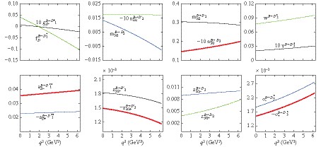
Figure 3. (color online) The q2 dependence of form factors for
${B\rightarrow}$ ${D^{*}_1}$ , D2,${D_2^{\prime}}$ , and${D^{*}_3}$ transitions.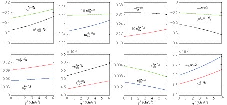
Figure 4. (color online) The q2 dependence of form factors for
${B_{s}\rightarrow}$ ${D^{*}_{s1}}$ ,${D_{s2}}$ , and${D_{s2}^{\prime}}$ ,${D^{*}_{s3}}$ transitions.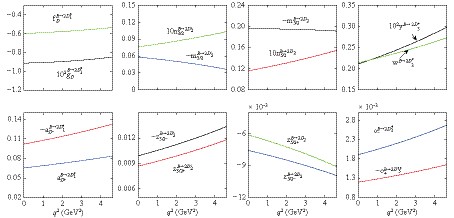
Figure 5. (color online) The q2 dependence of form factors for
${B\rightarrow}$ ${2D^{*}_1}$ ,${2D_2}$ ,${2D_2^{\prime}}$ , and${2D^{*}_3}$ transitions.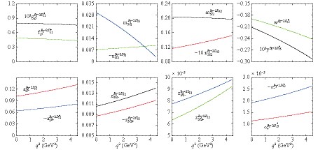
Figure 6. (color online) The q2 dependence of form factors for
${B_{s}\rightarrow}$ ${2D^{*}_{s1}}$ ,${2D_{s2}}$ ,${2D_{s2}^{\prime}}$ , and${2D^{*}_{s3}}$ transitions.${F(q^2=0)}$ 

${F(q^2_{\rm max})}$ 

${b_1}$ 

${b_2}$ 

${F(q^2=0)}$ 

${F(q^2_{\rm max})}$ 

${b_1}$ 

${b_2}$ 

${g_D^{B\rightarrow D_1^{*}}}$ 

0.0006 −0.0024 156.1 215.9 ${g_D^{B_{s}\rightarrow D_{s1}^{*}}}$ 

−0.0061 −0.0021 31.9 −41.3 ${f_D^{B\rightarrow D_1^{*}}}$ 

0.041 −0.104 92.36 925.3 ${f_D^{B_{s}\rightarrow D_{s1}^{*}}}$ 

−0.259 0.011 40.0 148.0 ${a_{D+}^{B\rightarrow D_1^{*}}}$ 

−0.023 −0.024 7.4 −21.4 ${a_{D+}^{B_{s}\rightarrow D_{s1}^{*}}}$ 

0.054 0.064 2.9 −17.8 ${a_{D-}^{B\rightarrow D_1^{*}}}$ 

0.035 0.039 6.2 −22.0 ${a_{D-}^{B_{s}\rightarrow D_{s1}^{*}}}$ 

−0.093 −0.116 1.2 −15.1
${n_{3/2}^{B\rightarrow D_2^{\prime}}}$ 

−0.00174 −0.00169 10.8 −42.8 ${n_{3/2}^{B_{s}\rightarrow D^{\prime}_{s2}}}$ 

0.0043 0.0049 4.8 −35.2 ${m_{3/2}^{B\rightarrow D_2^{\prime}}}$ 

0.013 −0.008 54.0 149.0 ${m_{3/2}^{B_{s}\rightarrow D^{\prime}_{s2}}}$ 

−0.027 0.021 69.8 −22.0 ${z_{3/2+}^{B\rightarrow D_2^{\prime}}}$ 

−0.0015 −0.0012 17.6 −70.6 ${z_{3/2+}^{B_{s}\rightarrow D^{\prime}_{s2}}}$ 

0.0044 0.0049 6.2 −41.8 ${z_{3/2-}^{B\rightarrow D_2^{\prime}}}$ 

0.0018 0.0016 14.2 −58.1 ${z_{3/2-}^{B_{s}\rightarrow D^{\prime}_{s2}}}$ 

−0.0052 −0.0059 5.2 −39.2
${n_{5/2}^{B\rightarrow D_2}}$ 

−0.015 −0.020 −2.2 −8.5 ${n_{5/2}^{B_{s}\rightarrow D_{s2}}}$ 

0.015 0.020 −2.9 −8.6 ${m_{5/2}^{B\rightarrow D_2}}$ 

0.304 0.286 11.4 −27.7 ${m_{5/2}^{B_{s}\rightarrow D_{s2}}}$ 

−0.327 −0.312 11.3 −36.2 ${z_{5/2+}^{B\rightarrow D_2}}$ 

0.0039 0.0078 −24.3 68.8 ${z_{5/2+}^{B_{s}\rightarrow D_{s2}}}$ 

−0.0043 −0.0082 −23.8 74.5 ${z_{5/2-}^{B\rightarrow D_2}}$ 

0.0089 0.0101 6.5 −62.7 ${z_{5/2-}^{B_{s}\rightarrow D_{s2}}}$ 

−0.010 −0.013 −0.56 −17.54
${y^{B\rightarrow D^{*}_3}}$ 

0.002 0.003 −6.85 7.00 ${y^{B_{s}\rightarrow D^{*}_{s3}}}$ 

−0.0021 −0.0031 −7.6 9.5 ${w^{B\rightarrow D^{*}_3}}$ 

0.077 0.095 2.1 −21.7 ${w^{B_{s}\rightarrow D^{*}_{s3}}}$ 

−0.101 −0.127 1.1 −22.5 ${o_{+}^{B\rightarrow D^{*}_3}}$ 

−0.0015 −0.0024 −8.1 20.0 ${o_{+}^{B_{s}\rightarrow D^{*}_{s3}}}$ 

0.0016 0.0023 −6.34 2.73 ${o_{-}^{B\rightarrow D^{*}_3}}$ 

0.0018 0.0028 −6.0 1.7 ${o_{-}^{B_{s}\rightarrow D^{*}_{s3}}}$ 

−0.0020 −0.0029 −6.9 4.5
${g_D^{B\rightarrow 2D_1^{*}}}$ 

−0.0095 −0.0087 15.5 −97.4 ${g_D^{B_{s}\rightarrow 2D_{s1}^{*}}}$ 

0.0079 0.0076 14.2 −91.4 ${f_D^{B\rightarrow 2D_1^{*}}}$ 

−0.631 −0.563 16.0 −49.0 ${f_D^{B_{s}\rightarrow 2D_{s1}^{*}}}$ 

0.491 0.438 16.5 −45.5 ${a_{D+}^{B\rightarrow 2D_1^{*}}}$ 

0.066 0.084 −3.4 −7.7 ${a_{D+}^{B_{s}\rightarrow 2D_{s1}^{*}}}$ 

−0.064 −0.082 −5.2 2.5 ${a_{D-}^{B\rightarrow 2D_1^{*}}}$ 

−0.102 −0.133 −4.8 −1.1 ${a_{D-}^{B_{s}\rightarrow 2D_{s1}^{*}}}$ 

0.101 0.132 −6.1 8.6
${n_{3/2}^{B\rightarrow 2D_2^{\prime}}}$ 

0.0076 0.0103 −8.3 17.9 ${n_{3/2}^{B_{s}\rightarrow 2D_{s2}^{\prime}}}$ 

−0.0074 −0.0099 −9.5 31.2 ${m_{3/2}^{B\rightarrow 2D_2^{\prime}}}$ 

−0.058 −0.036 30.6 −128.4 ${m_{3/2}^{B_{s}\rightarrow 2D_{s2}^{\prime}}}$ 

0.0296 0.0030 63.1 −198.2 ${z_{3/2+}^{B\rightarrow 2D_2^{\prime}}}$ 

0.0087 0.0118 −8.3 17.6 ${z_{3/2+}^{B_{s}\rightarrow 2D_{s2}^{\prime}}}$ 

−0.0087 −0.0117 −9.6 30.9 ${z_{3/2-}^{B\rightarrow 2D_2^{\prime}}}$ 

−0.010 −0.013 −7.7 12.9 ${z_{3/2-}^{B_{s}\rightarrow 2D_{s2}^{\prime}}}$ 

0.011 0.014 −8.7 22.6
${n_{5/2}^{B\rightarrow 2D_2}}$ 

0.0116 0.0154 −7.0 14.5 ${n_{5/2}^{B_{s}\rightarrow 2D_{s2}}}$ 

−0.0117 −0.0152 −7.1 18.9 ${m_{5/2}^{B\rightarrow 2D_2}}$ 

−0.196 −0.191 11.7 −43.4 ${m_{5/2}^{B_{s}\rightarrow 2D_{s2}}}$ 

0.203 0.197 12.2 −35.6 ${z_{5/2+}^{B\rightarrow 2D_2}}$ 

−0.0061 −0.0091 −15.5 53.0 ${z_{5/2+}^{B_{s}\rightarrow 2D_{s2}}}$ 

0.0064 0.0092 −15.9 55.2 ${z_{5/2-}^{B\rightarrow 2D_2}}$ 

−0.0076 −0.0099 −6.0 15.6 ${z_{5/2-}^{B_{s}\rightarrow 2D_{s2}}}$ 

0.0077 0.0098 −5.1 10.7
${y^{B\rightarrow 2D^{*}_3}}$ 

0.0021 0.0030 −11.2 35.0 ${y^{B_{s}\rightarrow 2D^{*}_{s3}}}$ 

−0.0021 −0.0029 −11.7 41.2 ${w^{B\rightarrow 2D^{*}_3}}$ 

0.214 0.273 −3.73 −5.3 ${w^{B_{s}\rightarrow 2D^{*}_{s3}}}$ 

−0.189 −0.241 −5.1 2.1 ${o_{+}^{B\rightarrow 2D^{*}_3}}$ 

−0.0012 −0.0016 −9.5 25.2 ${o_{+}^{B_{s}\rightarrow 2D^{*}_{s3}}}$ 

0.0011 0.0015 −9.5 28.2 ${o_{-}^{B\rightarrow 2D^{*}_3}}$ 

0.0019 0.0027 −10.6 30.0 ${o_{-}^{B_{s}\rightarrow 2D^{*}_{s3}}}$ 

−0.0019 −0.0026 −10.9 34.6 Table 4. Form factors for the semileptonic decays of
${B_{(s)}}$ to 1D- and 2D-wave D(s) mesons.With the above preparatory results, we perform numerical calculations of the branching ratios for the
$B_{(s)}$ semileptonic decays to D -wave$D/D_s$ mesons, which are listed in Table 5. The magnitudes of the branching ratios presented in Table 5 are expected to be typical values for$B_{(s)}$ decay to D -wave$D_{(s)}$ via semileptonic processes.Decay mode ${\ell=e}$ 

${\ell=\mu}$ 

${\ell=\tau}$ 

Decay mode ${\ell=e}$ 

${\ell=\mu}$ 

${\ell=\tau}$ 

${B\rightarrow D_1^{*}\ell\bar{\nu}_{\ell}}$ 

${6.62\times 10^{-5}}$ 

${6.53\times 10^{-5}}$ 

${1.35\times 10^{-6}}$ 

${B_{s}\rightarrow D_{s1}^{*}\ell\bar{\nu}_{\ell}}$ 

${1.97\times10^{-4}}$ 

${1.94\times10^{-4}}$ 

${2.37\times 10^{-6}}$ 

${B\rightarrow D^{\prime}_2\ell\bar{\nu}_{\ell}}$ 

${1.16\times10^{-6}}$ 

${1.14\times10^{-6}}$ 

${1.21\times10^{-8}}$ 

${B_{s}\rightarrow D^{\prime}_{s2}\ell\bar{\nu}_{\ell}}$ 

${1.07\times10^{-5}}$ 

${1.05\times10^{-5}}$ 

${1.04\times10^{-7}}$ 

${B\rightarrow D_2\ell\bar{\nu}_{\ell}}$ 

${5.39\times10^{-4}}$ 

${5.31\times10^{-4}}$ 

${7.40\times10^{-6}}$ 

${B_{s}\rightarrow D_{s2}\ell\bar{\nu}_{\ell}}$ 

${5.05\times10^{-4}}$ 

${4.97\times10^{-4}}$ 

${6.62\times10^{-6}}$ 

${B\rightarrow D^{*}_3\ell\bar{\nu}_{\ell}}$ 

${7.20\times10^{-5}}$ 

${7.08\times10^{-5}}$ 

${6.50\times10^{-7}}$ 

${B_{s}\rightarrow D^{*}_{s3}\ell\bar{\nu}_{\ell}}$ 

${1.13\times10^{-4}}$ 

${1.11\times10^{-4}}$ 

${8.78\times10^{-7}}$ 

${B\rightarrow 2D_1^{*}\ell\bar{\nu}_{\ell}}$ 

${7.86\times 10^{-5}}$ 

${7.73\times10^{-5}}$ 

${8.07\times10^{-7}}$ 

${B_{s}\rightarrow 2D_{s1}^{*}\ell\bar{\nu}_{\ell}}$ 

${6.37\times10^{-5}}$ 

${6.25\times10^{-5}}$ 

${3.76\times10^{-7}}$ 

${B\rightarrow 2D^{\prime}_2\ell\bar{\nu}_{\ell}}$ 

${8.77\times10^{-6}}$ 

${8.58\times10^{-6}}$ 

${7.55\times10^{-9}}$ 

${B_{s}\rightarrow 2D^{\prime}_{s2}\ell\bar{\nu}_{\ell}}$ 

${9.88\times10^{-6}}$ 

${9.65\times10^{-6}}$ 

${4.36\times10^{-9}}$ 

${B\rightarrow 2D_2\ell\bar{\nu}_{\ell}}$ 

${8.57\times10^{-5}}$ 

${8.40\times10^{-5}}$ 

${1.04\times10^{-7}}$ 

${B_{s}\rightarrow 2D_{s2}\ell\bar{\nu}_{\ell}}$ 

${7.02\times10^{-5}}$ 

${6.88\times10^{-5}}$ 

${6.16\times10^{-8}}$ 

${B\rightarrow 2D^{*}_3\ell\bar{\nu}_{\ell}}$ 

${1.63\times10^{-4}}$ 

${1.59\times10^{-4}}$ 

${8.64\times10^{-8}}$ 

${B_{s}\rightarrow 2D^{*}_{s3}\ell\bar{\nu}_{\ell}}$ 

${8.96\times10^{-5}}$ 

${8.74\times10^{-5}}$ 

${3.24\times10^{-8}}$ 

Table 5. Branching ratios for the B(s) semileptonic decay to 1D and 2D states of charmed/charmed-strange mesons.
We note that the production of D -wave charmed/charmed-strange via
$B_{(s)}$ semileptonic decay processes have also been studied by the QCD sum rule [65, 66] and the instantaneous Bethe-Salpeter method [51]. The results of these theoretical calculations are given in Table 6. Due to different sets of parameters and different approaches, there are discrepancies between different model calculations, so that the search for semileptonic decays relevant for the production of D -wave$D/D_s$ mesons will be an intriguing issue for future experiments.Decay mode Ref.[51] Ref. [66] Decay mode Ref.[51] Ref.[67] ${B\rightarrow D_1^*e\bar{\nu}_e}$ 

− ${6.0\times10^{-6}}$ 

${B_s\rightarrow D_{s1}^*e\bar{\nu}_e}$ 

− ${2.85\times10^{-7}}$ 

${B\rightarrow D_1^*\mu\bar{\nu}_{\mu}}$ 

− ${6.0\times10^{-6}}$ 

${B_s\rightarrow D_{s1}^*\mu\bar{\nu}_{\mu}}$ 

− ${2.85\times10^{-7}}$ 

${B\rightarrow D_1^*\tau\bar{\nu}_{\tau}}$ 

− − ${B_s\rightarrow D_{s1}^*\tau\bar{\nu}_{\tau}}$ 

− ${B\rightarrow D_2^{\prime}e\bar{\nu}_e}$ 

${4.1\times10^{-4}}$ 

${6.0\times10^{-6}}$ 

${B_s\rightarrow D_{s2}^{\prime}e\bar{\nu}_e}$ 

${5.2\times10^{-4}}$ 

${3.4\times10^{-7}}$ 

${B\rightarrow D_2^{\prime}\mu\bar{\nu}_{\mu}}$ 

${4.1\times10^{-4}}$ 

${6.0\times10^{-6}}$ 

${B_s\rightarrow D_{s2}^{\prime}\mu\bar{\nu}_{\mu}}$ 

${5.1\times10^{-4}}$ 

${3.4\times10^{-7}}$ 

${B\rightarrow D_2^{\prime}\tau\bar{\nu}_{\tau}}$ 

${2.7\times10^{-6}}$ 

− ${B_s\rightarrow D_{s2}^{\prime}\tau\bar{\nu}_{\tau}}$ 

${3.4\times10^{-6}}$ 

${B\rightarrow D_2e\bar{\nu}_e}$ 

${1.1\times10^{-3}}$ 

${1.5\times10^{-4}}$ 

${B_s\rightarrow D_{s2}e\bar{\nu}_e}$ 

${1.7\times10^{-3}}$ 

${1.02\times10^{-4}}$ 

${B\rightarrow D_2\mu\bar{\nu}_{\mu}}$ 

${1.1\times10^{-3}}$ 

${1.5\times10^{-4}}$ 

${B_s\rightarrow D_{s2}\mu\bar{\nu}_{\mu}}$ 

${1.7\times10^{-3}}$ 

${1.02\times10^{-4}}$ 

${B\rightarrow D_2\tau\bar{\nu}_{\tau}}$ 

${8.0\times10^{-6}}$ 

− ${B_s\rightarrow D_{s2}\tau\bar{\nu}_{\tau}}$ 

${1.4\times10^{-5}}$ 

${B\rightarrow D_3^*e\bar{\nu}_e}$ 

${1.0\times10^{-3}}$ 

${2.1\times10^{-4}}$ 

${B_s\rightarrow D_{s3}^*e\bar{\nu}_e}$ 

${1.5\times10^{-3}}$ 

${3.46\times10^{-4}}$ 

${B\rightarrow D_3^*\mu\bar{\nu}_{\mu}}$ 

${1.0\times10^{-3}}$ 

${2.1\times10^{-4}}$ 

${B_s\rightarrow D_{s3}^*\mu\bar{\nu}_{\mu}}$ 

${1.4\times10^{-3}}$ 

${3.46\times10^{-4}}$ 

${B\rightarrow D_3^*\tau\bar{\nu}_{\tau}}$ 

${5.4\times10^{-6}}$ 

− ${B_s\rightarrow D_{s3}^*\tau\bar{\nu}_{\tau}}$ 

${9.5\times10^{-6}}$ 

Table 6. Branching ratios for the semileptonic decay of 1D charmed (charmed-strange) meson produced via B meson obtained from various theoretical predictions.
-
For the processes discussed in this work, the transition amplitudes can be expressed using the deduced light-front form factors. Indeed, in the heavy quark limit, the light-front form factors can be related by Isgur-Wise (IW) functions
$\xi(\omega)$ and$\zeta(\omega)$ . The heavy-quark limit provides rigorous conditions for our calculations.The
$B_{(s)}\rightarrow D^{*}_{(s)1}$ and$B_{(s)}\rightarrow D^{\prime}_{(s)2}$ transitions in the heavy quark limit are related to the IW function$\xi(\omega)$ defined in Ref. [67] by the following equation:$ \begin{split} \xi(\omega)=&-\frac{6\sqrt{2}}{\sqrt{3}}\sqrt{m_Bm_D}\frac{1}{\omega-1}g_D(q^2)=\frac{-\sqrt{6}}{(\omega^2-1)\sqrt{m_Bm_D}}f_D(q^2)\\ &=-\frac{\sqrt{6m_B^3}}{3\sqrt{m_D}}(a_{D+}(q^2)+a_{D-}(q^2)) =\frac{\sqrt{6m_Bm_D}}{\omega+2}(a_{D+}(q^2)\\ &-a_{D-}(q^2))=2\sqrt{m_B^3m_D}n_{\frac{3}{2}}(q^2)=-\frac{1}{\omega-1}\sqrt{\frac{m_B}{m_D}}m_{\frac{3}{2}}(q^2)\\ &=\sqrt{m_B^3m_D}(z_{\frac{3}{2}+}(q^2)-z_{\frac{3}{2}-}(q^2)), \end{split} $

(1) and obey the additional HQS relation
$ z_{\frac{3}{2}+}(q^2)+z_{\frac{3}{2}-}(q^2)=0, $

(2) where
$\omega=(m_B^2+m_D^2-q^2)/(2m_Bm_D)$ .The
$B_{(s)}\rightarrow D_{(s)2}$ and$B_{(s)}\rightarrow D^{*}_{(s)3}$ transition form factors are related to the IW function$\zeta(\omega)$ by the following relations:$ \begin{split} \zeta(\omega)=&-\frac{5\sqrt{5}}{\sqrt{3}}\frac{\sqrt{m_B^3 m_D}}{\omega+1}n_{5\over2}(q^2)=-\frac{5}{2}\sqrt{\frac{5}{3}}\sqrt{\frac{m_B}{m_D}}\frac{1}{1-\omega^2}m_{\frac{5}{2}}(q^2)\\ &=\frac{m_B^5}{m_D}\sqrt{\frac{5}{3}}(z_{\frac{5}{2}+}(q^2)+z_{\frac{5}{2}-}(q^2))=5\sqrt{\frac{5}{3}}\sqrt{m_B^3m_D}\\& \frac{1}{3-2\omega} (z_{\frac{5}{2}+}(q^2)-z_{\frac{5}{2}-}(q^2))=2y(q^2)\sqrt{m_B^5m_D}\\ &=\sqrt{\frac{m_B^3}{m_D}}\frac{w(q^2)}{\omega+1}=-\sqrt{\frac{m_B^7}{m_D}}(o_{+}(q^2)-o_{-}(q^2)), \end{split} $

(3) and
$ o_{+}(q^2)+o_{-}(q^2)=0. $

(4) These relations are model independent, which is the consequence of heavy quark symmetry. In the following, we will check whether our results obtained from the light-front quark model satisfy these relations.
To present our numerical results, we rewrite Eq. (52) and Eq. (54) as
$\begin{split} \xi=&\xi_{(g_D)}=\xi_{(f_D)}=\xi_{(a_{D+}+a_{D-})}=\xi_{(a_{D+}-a_{D-})}\\ =&\xi_{(n_{3/2})}=\xi_{(m_{3/2})}=\xi_{(z_{3/2+}-z_{3/2-})}, \end{split}$

and
$\begin{split} \zeta=&\zeta_{(n_{5/2})}=\zeta_{(m_{5/2})}=\zeta_{(z_{5/2+}+z_{5/2-})}=\zeta_{(z_{5/2+}-z_{5/2-})}\\ =&\zeta_{(y)}=\zeta_{(w)}=\zeta_{(o_+-o_-)}. \end{split} $

For example, in Eq. (5),
$ \xi_{(g_D)}\equiv -\frac{6\sqrt{2}}{\sqrt{3}}\sqrt{m_Bm_D}\frac{1}{\omega-1}g_D(q^2), $

(7) $ \xi_{(f_D)}\equiv \frac{-\sqrt{6}}{(\omega^2-1)\sqrt{m_Bm_D}}f_D(q^2). $

(8) Other
$\xi_{(F)}$ terms correspond to the expressions given in Eq. (52). The same notation is also used in Eq. (54) and Eq. (57). Using the above notation, we present the numerical results for IW functions for$B_{(s)}\rightarrow 1D^*_{(s)1} (2D^*_{(s)1}), $ $ 1D^{(\prime)}_{(s)2} (2D^{(\prime)}_{(s)2}), 1D^*_{(s)3} (2D^*_{(s)3})$ light-front form factors in Table 7.In Table 7, we present the calculated IW function values for
$q^2=0$ and$q^2=q^2_{\rm max}$ . We give the results for$B\rightarrow $ $1D^*_{1}, 1D^{(\prime)}_{2}, 1D^*_{3}$ processes, the results for$B\rightarrow 2D^*_{1}, 2D^{(\prime)}_{2}, 2D^*_{3}$ and$B_s\rightarrow 1D^*_{s1}(2D^*_{s1}),$ $ 1D^{(\prime)}_{s2}(2D^{(\prime)}_{s2}), 1D^*_{s3}(2D^*_{s3}) $ can be obtained in a similar way. From Table 7, we find that$\xi_{(g_D)}$ ,$\xi_{(f_D)}$ ,$\xi_{(a_{D+}+a_{D-})}$ ,$\xi_{n_{3/2}}$ ,$\xi_{m_{3/2}}$ and$\xi_{(z_{3/2+}-z_{3/2-})}$ are similar and approximately meet the requirement of Eq. (52). In addition,$z_{3/2+}$ has an opposite sign to that of$z_{3/2-}$ , which is approximately satisfied in Table 7. However, the value of$\xi_{(a_{D+}-a_{D-})}$ is about two times larger than the other$\xi$ form factors, which implies a violation of Eq. (52). The transition form factors in$B\rightarrow D_2$ and$B\rightarrow D^*_3$ processes can be related by IW function$\zeta$ . We find that the numerical results of$\zeta_{n_{5/2}}$ ,$\zeta_{(y)}$ ,$\zeta_{(w)}$ , and$\zeta_{(o_+-o_-)}$ are close, so that the relation in Eq. (55) for the form factors$o_+(q^2)$ and$o_{-}(q^2)$ holds. We also find a discrepancy in the$\zeta_{(m_{5/2})}$ function, which is about 2-3 times larger than the other$\zeta$ functions.Indeed, from Table 7 we note that discrepancies between the results obtained in the light-front quark model and the expectations from the heavy quark limit also exist in
$B\rightarrow 2D^*_{1}, 2D^{(\prime)}_{2}, 2D^*_{3}$ and$B_s\rightarrow 1D^*_{s1}(2D^*_{s1}),$ $ 1D^{(\prime)}_{s2}(2D^{(\prime)}_{s2}), 1D^*_{s3}(2D^*_{s3})$ transition processes. We point out that the relations in Eqs. (52)-(55) were derived in the heavy quark limit, while in our calculations we introduced definite masses for$c$ and$b$ quarks, which could indicate that the$1/m_Q$ correction could play an essential role for some form factors.${q^2=0}$ 

${q^2=q_{\rm max}^2}$ 

${q^2=0}$ 

${q^2=q_{\rm max}^2}$ 

${q^2=0}$ 

${q^2=q_{\rm max}^2}$ 

${q^2=0}$ 

${q^2=q_{\rm max}^2}$ 

${\xi_{(g_D)}^{B\rightarrow D^*_1}}$ 

0.051 ... ${\zeta_{(n_{5/2})}^{B\rightarrow D^{\prime}_2}}$ 

0.85 1.27 ${\xi_{(g_D)}^{B\rightarrow 2D^*_1}}$ 

1.27 ... ${\zeta_{(n_{5/2})}^{B\rightarrow 2D^{\prime}_2}}$ 

0.75 1.05 ${\xi_{(f_D)}^{B\rightarrow D^*_1}}$ 

0.053 ... ${\zeta_{(m_{5/2})}^{B\rightarrow D^{\prime}_2}}$ 

2.81 ... ${\xi_{(f_D)}^{B\rightarrow 2D^*_1}}$ 

1.18 ... ${\zeta_{(m_{5/2})}^{B\rightarrow 2D^{\prime}_2}}$ 

2.68 ... ${\xi_{(a_{D+}+a_{D-})}^{B\rightarrow D^*_1}}$ 

0.076 0.088 ${\zeta_{(z_{{5/2+} }+z_{{5/2-}})}^{B\rightarrow D^{\prime}_2}}$ 

0.66 0.98 ${\xi_{(a_{D+}+a_{D-})}^{B\rightarrow 2D^*_1}}$ 

0.21 0.27 ${\zeta_{(z_{{5/2+} }+z_{{5/2-}})}^{B\rightarrow 2D^{\prime}_2}}$ 

0.63 0.86 ${\xi_{(a_{D+}-a_{D-})}^{B\rightarrow D^*_1}}$ 

0.168 0.198 ${\xi_{(a_{D+}-a_{D-})}^{B\rightarrow 2D^*_1}}$ 

0.53 0.72
${\xi_{(n_{3/2})}^{B\rightarrow D^{\prime}_2}}$ 

0.070 0.068 ${\zeta_{(y)}^{B\rightarrow D^*_3}}$ 

0.43 0.64 ${\xi_{(n_{3/2})}^{B\rightarrow 2D^{\prime}_2}}$ 

0.33 0.44 ${\zeta_{(y)}^{B\rightarrow 2D^*_3}}$ 

0.48 0.67 ${\xi_{(m_{3/2})}^{B\rightarrow D^{\prime}_2}}$ 

0.086 ... ${\zeta_{(w)}^{B\rightarrow D^*_3}}$ 

0.25 0.35 ${\xi_{(m_{3/2})}^{B\rightarrow 2D^{\prime}_2}}$ 

0.53 ... ${\zeta_{(w)}^{B\rightarrow 2D^*_3}}$ 

0.69 0.93 ${\xi_{(z_{{3/2+}}-z_{{3/2-}})}^{B\rightarrow D^{\prime}_2}}$ 

0.067 0.056 ${\zeta_{(o_{+}-o_{-})}^{B\rightarrow D^*_3}}$ 

0.68 1.00 ${\xi_{(z_{{3/2+}}-z_{{3/2-}})}^{B\rightarrow 2D^{\prime}_2}}$ 

0.40 0.54 ${\zeta_{(o_{+}-o_{-})}^{B\rightarrow 2D^*_3}}$ 

0.59 0.83 ${z_{{3/2+}}}$ 

0.0015 0.0012 ${o_{+}}$ 

−0.0015 −0.0024 ${z_{{3/2+}}}$ 

−0.0086 −0.0117 ${o_{+}}$ 

−0.0012 −0.0016 ${z_{{3/2-}}}$ 

−0.0018 −0.0016 ${o_{-}}$ 

0.0019 0.0028 ${z_{{3/2-}}}$ 

0.0099 0.0134 ${o_{-}}$ 

0.0019 0.0027
${\xi_{(g_D)}^{B_s\rightarrow D^*_{s1}}}$ 

0.58 ... ${\zeta_{(n_{5/2})}^{B_s\rightarrow D^{\prime}_{s2}}}$ 

0.92 1.37 ${\xi_{(g_D)}^{B_s\rightarrow 2D^*_{s1}}}$ 

1.23 ... ${\zeta_{(n_{5/2})}^{B_s\rightarrow 2D^{\prime}_{s2}}}$ 

0.79 1.08 ${\xi_{(f_D)}^{B_s\rightarrow D^*_{s1}}}$ 

0.36 ... ${\zeta_{(m_{5/2})}^{B_s\rightarrow D^{\prime}_{s2}}}$ 

3.21 ... ${\xi_{(f_D)}^{B_s\rightarrow 2D^*_{s1}}}$ 

1.02 ... ${\zeta_{(m_{5/2})}^{B_s\rightarrow 2D^{\prime}_{s2}}}$ 

3.01 ... ${\xi_{(a_{D+}+a_{D-})}^{B_s\rightarrow D^*_{s1}}}$ 

0.23 0.31 ${\zeta_{(z_{{5/2+}}+z_{{5/2-}})}^{B_s\rightarrow D^{\prime}_{s2}}}$ 

0.73 1.07 ${\xi_{(a_{D+}+a_{D-})}^{B_s\rightarrow 2D^*_{s1}}}$ 

0.21 0.28 ${\zeta_{(z_{{5/2+} }+z_{{5/2-}})}^{B_s\rightarrow 2D^{\prime}_{s2}}}$ 

0.67 0.90 ${\xi_{(a_{D+}-a_{D-})}^{B_s\rightarrow D^*_{s1}}}$ 

0.44 0.58 ${\xi_{(a_{D+}-a_{D-})}^{B_s\rightarrow 2D^*_{s1}}}$ 

0.54 0.72
${\xi_{(n_{3/2})}^{B_s\rightarrow D^{\prime}_{s2}}}$ 

0.18 0.21 ${\zeta_{(y)}^{B_s\rightarrow D^*_{s3}}}$ 

0.48 0.71 ${\xi_{(n_{3/2})}^{B_s\rightarrow 2D^{\prime}_{s2}}}$ 

0.33 0.44 ${\zeta_{(y)}^{B_s\rightarrow 2D^*_{s3}}}$ 

0.51 0.70 ${\xi_{(m_{3/2})}^{B_s\rightarrow D^{\prime}_{s2}}}$ 

0.18 ... ${\zeta_{(w)}^{B_s\rightarrow D^*_{s3}}}$ 

0.34 0.47 ${\xi_{(m_{3/2})}^{B_s\rightarrow 2D^{\prime}_{s2}}}$ 

0.29 ... ${\zeta_{(w)}^{B_s\rightarrow 2D^*_{s3}}}$ 

0.61 0.83 ${\xi_{(z_{{3/2+}}-z_{{3/2-}})}^{B_s\rightarrow D^{\prime}_{s2}}}$ 

0.20 0.23 ${\zeta_{(o_{+}-o_{-})}^{B_s\rightarrow D^*_{s3}}}$ 

0.74 1.09 ${\xi_{(z_{{3/2+}}-z_{{3/2-}})}^{B_s\rightarrow 2D^{\prime}_{s2}}}$ 

0.43 0.57 ${\zeta_{(o_{+}-o_{-})}^{B_s\rightarrow 2D^*_{s3}}}$ 

0.61 0.82 ${z_{{3/2+}}}$ 

0.0044 0.0049 ${o_{+}}$ 

0.0016 0.0023 ${z_{{3/2+}}}$ 

−0.0086 −0.0115 ${o_{+}}$ 

0.0011 0.0015 ${z_{{3/2-}}}$ 

−0.0052 −0.0059 ${o_{-}}$ 

−0.0020 −0.0029 ${z_{{3/2-}}}$ 

0.0105 0.0140 ${o_{-}}$ 

−0.0019 −0.0026 Table 7. The IW functions for the light-front quark model for q2=0 and
${q^2=q^2_{\rm max}}$ . -
In the past several years, considerable progress has been achieved in observing
$D$ -wave$D/D_s$ mesons in various experiments [2-5]. These observations enrich the$D/D_s$ meson families. Although all candidates for$D$ -wave$D/D_s$ are produced in nonleptonic weak decays of$B/B_s$ mesons, we studied in this work the possibility of producing$1D$ and$2D$ $D/D_s$ meson families via semileptonic decays, although$2D$ states of$D/D_s$ meson families have not yet been experimentally observed.In order to get numerical results for semileptonic decays, we adopted the light-front quark model, which has been extensively applied in the studies of decay processes including semileptonic decays [35-48]. Our study in the framework of LFQM shows that the analysis of the production of the relevant D -wave
$D/D_s$ mesons via$B/B_s$ mesons is much more complicated than the analysis of$S$ -wave and$P$ -wave$D/D_s$ mesons [35-37]. We have given detailed derivation of many formulas necessary for obtaining the final semileptonic decay widths. The numerical results obtained show that the semileptonic decays of$B/B_s$ mesons are suitable for searching for$D$ -wave charmed and charmed-strange mesons. Furthermore, we have shown that our light-front form factors approximately satisfy HQS requirements.Theoretical studies of the
$B_{(s)}$ semileptonic decays to D -wave charmed mesons were performed in the past using the QCD sum rule [65, 66] and the instantaneous Bethe-Salpeter method [51]. We have noted that different theoretical groups have given different results for the$B_{(s)}$ semileptonic decays to D -wave charmed mesons. Thus, experimental search for semileptonic decays predicted by our results could provide a crucial test for the theoretical frameworks for studying$B_{(s)}$ semileptonic decays.As indicated by our numerical results, semileptonic decays of pseudoscalar
$B/B_s$ mesons could be the ideal platform for investigating D -wave charmed and charmed-strange mesons. With the LHCb continuing to take data at 13 TeV and the forthcoming run of Belle-II, we expect further experimental progress.Kan Chen would like to thank Qi Huang and Hao Xu for helpful discussion. We also would like to thank Yu-Ming Wang for the suggestion of form factors adopted in this work.
-
In this Appendix, we present the detailed expansions of
$\hat{S}_{\mu\nu}^{{}^3D_1}$ ,$\hat{S}_{\mu\alpha\beta}^{{}^1D_2}$ ,$\hat{S}_{\mu\alpha\beta}^{{}^3D_2}$ and$\hat{S}^{{}^3D_3}_{\mu\alpha\beta\nu}$ . Form factors associated with these expressions are also given.When integrating over
$p_1^{\prime-}$ , we need to do the following integrations$ \tag{A1} \hat{B}^{B_{(s)}(D^{*}_{(s)1})}_{\mu}=\frac{N_c}{16\pi^3}\int_0^{1}{\rm d}x\int {\rm d}^2p^{\prime}_{\bot}\frac{h^{\prime}_0h^{\prime\prime}_{{}^3D_1}}{\left(1-x\right)N^{\prime}_1N^{\prime\prime}_1}\hat{S}^{{}^3D_1}_{\mu\nu}\epsilon^{*\prime\prime\nu}, $

$ \tag{A2} \hat{B}^{B_{(s)}(D^{*}_{(s)2})}_{\mu}=\frac{N_c}{16\pi^3}\int_0^{1}{\rm d}x\int {\rm d}^2p^{\prime}_{\bot}\frac{h^{\prime}_0h^{\prime\prime}_{{}^1D_2}}{\left(1-x\right)N^{\prime}_1N^{\prime\prime}_1} \hat{S}^{{}^1D_2}_{\mu\alpha\beta}\epsilon^{*\prime\prime\alpha\beta}. $

$ \tag{A3} \hat{B}^{B_{(s)}(D_{(s)2}^{*\prime})}_{\mu}=\frac{N_c}{16\pi^3}\int_0^{1}{\rm d}x\int {\rm d}^2p^{\prime}_{\bot}\frac{h^{\prime}_0h^{\prime\prime}_{{}^3D_2}}{\left(1-x\right)N^{\prime}_1N^{\prime\prime}_1} \hat{S}^{{}^3D_2}_{\mu\alpha\beta}\epsilon^{*\prime\prime\alpha\beta}, $

$ \tag{A4} \hat{B}^{B_{(s)}(D^{*}_{(s)3})}_{\mu}=\frac{N_c}{16\pi^3}\int_0^{1}{\rm d}x\int {\rm d}^2p'_{\bot}\frac{h'_0h'_{{}^3D_3}}{(1-x)N'_1N''_1}\hat{S}^{{}^3D_3}_{\mu\alpha\beta\nu}\epsilon''^{*\alpha\beta\nu}, $

where the trace expansions of
$\hat{S}_{\mu\nu}^{{}^3D_1}$ ,$\hat{S}_{\mu\alpha\beta}^{{}^1D_2}$ ,$\hat{S}_{\mu\alpha\beta}^{{}^3D_2}$ and$\hat{S}^{{}^3D_3}_{\mu\alpha\beta\nu}$ are$ \tag{A5} \begin{split} \hat{S}_{\mu\nu}^{{}^3D_1}=&{\rm Tr}\left\{\left[\gamma_{\nu}-\frac{1}{\omega^{\prime\prime}_{{}^3D_1}}\left(p^{\prime\prime}_1-p_2\right)_{\nu}\right] \left({\not \!\!{p}}^{\prime\prime}_{1}+m^{\prime\prime}_1\right)\gamma_{\mu}\left(1-\gamma_5\right) \left({\not \!\!{p}}^{\prime}_1+m^{\prime}_1\right)\gamma_5\left(-{\not \!\!{p}}_2+m_2\right)\right\}\\ =&-2i\epsilon_{\mu\nu\alpha\beta}\left[p_1^{\prime\alpha}P^{\beta} \left(m_1^{\prime\prime}-m_1^{\prime}\right)+p_1^{\prime\alpha}q^{\beta} \left(m_1^{\prime\prime}+m_1^{\prime}-2m_2\right)+q^{\alpha}P^{\beta}m_1^{\prime}\right] +\frac{1}{\omega^{\prime\prime}_{{}^3D_1}}\left(4p_{1\nu}^{\prime}-3q_{\nu}-P_{\nu}\right)\\&\times i\epsilon_{\mu\alpha\beta\rho}p_1^{\prime\alpha}q^{\beta}P^{\rho}+2g_{\mu\nu} \left[m_2\left(q^2-N_1^{\prime}-N_1^{\prime\prime}-m_1^{\prime2}-m_1^{\prime\prime2}\right)- m_1^{\prime}\left(M^{\prime\prime2}-N_1^{\prime\prime}-N_2-m_1^{\prime\prime2} -m_2^{2}\right)\right.\\&\left.-m_1^{\prime\prime}\left(M^{\prime2}-N_1^{\prime}-N_2-m_1^{\prime2} -m_2^{2}\right)-2m_1^{\prime}m_1^{\prime\prime}m_2\right]+8p_{1\mu}^{\prime}p_{1\nu}^{\prime} \left(m_2-m_1^{\prime}\right)-2\left(P_{\mu}q_{\nu}+q_{\mu}P_{\nu}+2q_{\mu}q_{\nu}\right)m_1^{\prime}\\& +2p_{1\mu}^{\prime}P_{\nu}\left(m_1^{\prime}-m_1^{\prime\prime}\right)+2p_{1\mu}^{\prime} q_{\nu}\left(3m_1^{\prime}-m_1^{\prime\prime}-2m_2\right)+2P_{\mu}p_{1\nu}^{\prime} \left(m_1^{\prime}+m_1^{\prime\prime}\right)+2q_{\mu}p_{1\nu}^{\prime}\left(3m_1^{\prime} +m_1^{\prime\prime}-2m_2\right)\\&+\frac{1}{2\omega^{\prime\prime}_{{}^3D_1}}\left(4p_{1\nu}^{\prime}-3q_{\nu}-P_{\nu}\right) \left\{2p_{1\mu}^{\prime}\left[M^{\prime2}+M^{\prime\prime2}-q^2-2N_2+ 2\left(m_1^{\prime}-m_2\right)\left(m_1^{\prime\prime}+m_2\right)\right]\right.\\&\left.+q_{\mu}\left[q^2-2M^{\prime2} +N_1^{\prime}-N_1^{\prime\prime}+2N_2-\left(m_1^{\prime}+m_1^{\prime\prime}\right)^2+ 2\left(m_1^{\prime}-m_2\right)^2\right]+P_{\mu}\left[q^2-N_1^{\prime}- N_1^{\prime\prime}-\left(m_1^{\prime}+m_1^{\prime\prime}\right)^2\right]\right\}, \end{split} $

$ \tag{A6} \begin{split} \hat{S}_{\mu\alpha\beta}^{{}^1D_2}=&{\rm Tr}\left\{\left[\gamma_5 \frac{\left(p_2-p_1^{\prime\prime}\right)_{\alpha}}{2}\frac{\left(p_2-p_1^{\prime\prime}\right)_{\beta}}{2}\right]\left({\not \!\!{p}}^{\prime\prime}_{1} +m^{\prime\prime}_1\right)\gamma_{\mu}\left(1-\gamma_5\right) \left({\not \!\!{p}}^{\prime}_1+m^{\prime}_1\right)\gamma_5\left(-{\not \!\!{p}}_2+m_2\right)\right\}\\ =&-\frac{1}{8}i\epsilon_{\mu\nu\sigma\delta}\left(P_{\alpha}-4p^{\prime}_{1\alpha}+3q_{\alpha}\right) \left(P_{\beta}-4p^{\prime}_{1\beta}+3q_{\beta}\right)P^{\nu}p^{\prime\sigma}_1q^{\delta}- \left\{\frac{1}{16}\left(P_{\alpha}-4p^{\prime}_{1\alpha}+3q_{\alpha}\right)\right.\\&\left.\times\left(P_{\beta}-4p^{\prime}_{1\beta}+3q_{\beta}\right) \left[-q_{\mu}\left(2m_2^2-4m_2m^{\prime}_1-m^{\prime\prime2}_1+2m^{\prime}_1m^{\prime\prime}_1+m^{\prime2}_1-2M^{\prime2}+2N_2-N^{\prime\prime}_1 +N^{\prime}_1+q^2\right)\right.\right.\\&\left.\left.+2p^{\prime}_{1\mu}\left[2\left(m_2-m^{\prime\prime}_1\right)\left(m_2-m^{\prime}_1\right)-M^{\prime\prime2} -M^{\prime2}+2N_2+q^2\right]+P_{\mu} \left[\left(m^{\prime\prime}_1-m^{\prime}_1\right)^2+N^{\prime\prime}_1+N^{\prime}_1-q^2\right]\right]\right\}, \end{split} $

$ \tag{A7} \begin{split} \hat{S}_{\mu\alpha\beta}^{{}^3D_2}=&{\rm Tr}\left\{\gamma_5 \left[\frac{1}{\omega_{{}^3D_2}^{a\prime\prime}}\gamma_{\alpha}\gamma_{\beta}+\frac{1}{\omega_{{}^3D_2}^{b\prime\prime}} \gamma_{\alpha}\frac{\left(p_2-p^{\prime\prime}_1\right)_{\beta}}{2}+\frac{1}{\omega_{{}^3D_2}^{c\prime\prime}}\frac{\left(p_2-p^{\prime\prime}_1\right)_{\alpha}}{2} \frac{\left(p_2-p^{\prime\prime}_1\right)_{\beta}}{2}\right]\right.\\&\left. \times\left({\not \!\!{p}}^{\prime\prime}_{1}+m^{\prime\prime}_1\right)\gamma_{\mu}\left(1-\gamma_5\right) \left({\not \!\!{p}}^{\prime}_1+m^{\prime}_1\right)\gamma_5\left(-{\not \!\!{p}}_2+m_2\right)\right\}\\ &=-i\frac{1}{2\omega^{b\prime\prime}_{{}^3D_2}}\epsilon_{\alpha\mu\sigma\delta} \left(P_{\beta}-4p^{\prime}_{1\beta}+3q_{\beta}\right)\left\{\left(m^{\prime}_1+m^{\prime\prime}_1\right)P^{\sigma}p^{\prime\delta}_1- q^{\delta}\left[p^{\prime\sigma}_1(2m_2+m^{\prime\prime}_1-m^{\prime}_1)+m^{\prime}_1P^{\sigma}\right]\right\}\\& -\frac{i}{8\omega^{c\prime\prime}_{{}^3D_2}}\epsilon_{\mu\lambda\sigma\delta} P^{\lambda}p^{\prime\sigma}_1q^{\delta}\left(P_{\alpha}-4p^{\prime}_{1\alpha}+3q_{\alpha}\right) \left(P_{\beta}-4p^{\prime}_{1\beta}+3q_{\beta}\right)-\frac{1}{2\omega^{b\prime\prime}_{{}^3D_2}}\left(P_{\beta}-4p^{\prime}_{1\beta}+3q_{\beta}\right)\\&\times \left\{g_{\alpha\mu}\left[m_2^2\left(m^{\prime\prime}_1-m^{\prime}_1\right)+m_2\left(\left(m^{\prime\prime}_1-m^{\prime}_1\right)^2+N^{\prime\prime}_1 +N^{\prime}_1-q^2\right)-m^{\prime\prime2}_1m^{\prime}_1 +m^{\prime\prime}_1\left(m^{\prime2}_1-M^{\prime2}+Z_2+N^{\prime}_1\right)\right.\right.\\&\left.\left. +m^{\prime}_1\left(M^{\prime\prime2}-Z_2-N^{\prime\prime}_1\right)\right]+p^{\prime}_{1\alpha}\left[q_{\mu}\left(2m_2+m^{\prime\prime}_1-3m^{\prime}_1\right) +4\left(m^{\prime}_1-m_2\right)p^{\prime}_{1\mu} +\left(m^{\prime\prime}_1-m^{\prime}_1\right)P_{\mu}\right]\right.\\&\left.+2m_2p^{\prime}_{1\mu}q_{\alpha}-m^{\prime\prime}_1 \left(P_{\alpha}p^{\prime}_{1\mu} +p^{\prime}_{1\mu}q_{\alpha}\right)+m^{\prime}_1\left[-P_{\alpha}p^{\prime}_{1\mu}+P_{\mu}q_{\alpha} +q_{\mu}(P_{\alpha}+2q_{\alpha})-3p^{\prime}_{1\mu}q_{\alpha}\right]\right\}\\& -\frac{1}{16\omega^{c\prime\prime}_{{}^3D_2}}\left(P_{\alpha}-4p^{\prime}_{1\alpha}+3q_{\alpha}\right) \left(P_{\beta}-4p^{\prime}_{1\beta}+3q_{\beta}\right)\left\{-q_{\mu}\left(2m_2^2-4m_2m^{\prime}_1-m^{\prime\prime2}_1+ 2m^{\prime\prime}_1m^{\prime}_1+m^{\prime2}_1\right.\right.\\&\left.-2M^{\prime2}+2Z_2-N^{\prime\prime}_1+ N^{\prime}_1+q^2\right)+2p^{\prime}_{1\mu} \left[2(m_2-m^{\prime\prime}_1)(m_2-m^{\prime}_1) -M^{\prime\prime2}-M^{\prime2}+2Z_2+q^2\right]\\&\left.+P_{\mu}\left[\left(m^{\prime\prime}_1-m^{\prime}_1\right)^2 +N^{\prime\prime}_1+N^{\prime}_1-q^2\right]\right\}, \end{split} $

$ \tag{A8} \begin{split} \hat{S}^{{}^3D_3}_{\mu\alpha\beta\nu}=& {\rm Tr}\left\{\left[\frac{\left(p_2-p^{\prime\prime}_1\right)_{\alpha}}{2}\frac{\left(p_2-p^{\prime\prime}_1\right)_{\beta}}{2} \left(\gamma_\nu+\frac{\left(p_2-p^{\prime\prime}_1\right)_{\nu}}{\omega^{\prime\prime}_{{}^3D_3}}\right) +\frac{\left(p_2-p^{\prime\prime}_1\right)_{\alpha}}{2}\frac{\left(p_2-p^{\prime\prime}_1\right)_{\nu}}{2}(\gamma_\beta+ \frac{\left(p_2-p^{\prime\prime}_1\right)_{\beta}}{\omega^{\prime\prime}_{{}^3D_3}})\right.\right.\\&\left.\left. +\frac{\left(p_2-p^{\prime\prime}_1\right)_{\nu}}{2}\frac{\left(p_2-p^{\prime\prime}_1\right)_{\beta}}{2}\left(\gamma_\alpha +\frac{\left(p_2-p^{\prime\prime}_1\right)_{\alpha}}{\omega^{\prime\prime}_{{}^3D_3}}\right)\right] \left({\not \!\!{p}}^{\prime\prime}_{1}+m^{\prime\prime}_1\right)\gamma_{\mu}\left(1-\gamma_5\right) \left({\not \!\!{p}}^{\prime}_1+m^{\prime}_1\right)\gamma_5\left(-{\not \!\!{p}}_2+m_2\right)\right\}\\ &=-\frac{3i}{8}\epsilon _{\mu\nu\sigma\delta}\left(P_{\alpha}-4p^{\prime}_{1\alpha}+3q_{\alpha}\right)\left(P_{\beta}-4p^{\prime}_{1\beta}+3q_{\beta}\right) \left\{q^{\delta}\left[m^{\prime}_1P^{\sigma}-p^{\prime\sigma}_{1}(-2m_2+m^{\prime\prime}_1+m^{\prime}_1)\right]+\left(m^{\prime\prime}_1-m^{\prime}_1\right) P^{\sigma}p^{\prime\delta} _{1}\right\}\\&+\frac{3i}{16\omega^{\prime\prime}_{{}^3D_3}}\epsilon_{\mu\sigma\delta\lambda}P^{\sigma}p^{\prime\delta}_1 q^{\lambda}\left(P_{\alpha}-4p^{\prime}_{1\alpha}+3q_{\alpha}\right)\left(P_{\beta}-4p^{\prime}_{1\beta}+3q_{\beta}\right)\left(P_{\nu}-4p^{\prime}_{1\nu}+3q_{\nu}\right) +\frac{3}{8}\left(P_\alpha-4p^{\prime}_{1\alpha}+3q_{\alpha}\right)\\&\times\left(P_{\beta}-4p^{\prime}_{1\beta}+3q_{\beta}\right) \left\{g_{\mu\nu}\left[m_2^2\left(m^{\prime\prime}_1+m^{\prime}_1\right)-m_2\left[\left(m^{\prime\prime}_1+m^{\prime}_1\right)^2+N^{\prime\prime}_1+N^{\prime}_1-q^2\right] +m^{\prime\prime2}_1m^{\prime}_1+m^{\prime\prime}_1\left(m^{\prime2}_1-M^{\prime2}+Z_2+N^{\prime}_1\right)\right.\right.\\&\left.\left.+ m^{\prime}_1\left(-M^{\prime\prime2}+Z_2+N^{\prime\prime}_1\right)\right]+p^{\prime}_{1\mu}\left[-q_{\nu}(2m_2+m^{\prime\prime}_1-3m^{\prime}_1)+ 4(m_2-m^{\prime}_1)p^{\prime}_{1\nu}+ (m^{\prime}_1-m^{\prime\prime}_1)P_{\nu}\right]-2m_2p^{\prime}_{1\nu}q_{\mu}+m^{\prime\prime}_1\left(P_{\mu}p^{\prime}_{1\nu}\right.\right.\\& \left.\left. +p^{\prime}_{1\nu}q_{\mu}\right)+m^{\prime}_1\left(P_{\mu}p^{\prime}_{1\nu}-P_{\nu}q_{\mu}-q_{\nu}P_{\mu}-2q_{\nu}q_{\mu}+3p^{\prime}_{1\nu}q_{\mu}\right)\right\}+ \frac{3}{32\omega^{\prime\prime}_{{}^3D_3}}\left(P_{\alpha}-4p^{\prime}_{1\alpha}+3q_{\alpha}\right)\left(P_{\beta}-4p^{\prime}_{1\beta}+3q_{\beta}\right)\\&\times \left(P_{\nu}-4p^{\prime}_{1\nu}+3q_{\nu}\right)\left\{-q_{\mu}\left[2m_2^2-2m^{\prime}_1\left(2m_2+m^{\prime\prime}_1\right)-m^{\prime\prime2}_1+m^{\prime2}_1-2M^{\prime2}+2Z_2 -N^{\prime\prime}_1+N^{\prime}_1+q^2\right]\right.\\&\left.+ 2p^{\prime}_{1\mu}\left[2(m_2+m^{\prime\prime}_1)\left(m_2-m^{\prime}_1\right)-M^{\prime\prime2}-M^{\prime2}+2Z_2+q^2\right]+P_{\mu}\left[\left(m^{\prime\prime}_1+m^{\prime}_1\right)^2 +N^{\prime\prime}_1+N^{\prime}_1-q^2\right]\right\}. \end{split} $

The corresponding form factors for the
${}^1D_2$ state are$\tag{A9} n(q^2)=\frac{N_c}{16\pi^3}\int {\rm d}x_2 {\rm d}^2 p^{\prime}_{\bot}\frac{4h^{\prime}_Ph^{\prime\prime}_{{}^1D_2}}{(1-x)\hat{N}_1^{\prime}\hat{N}_1^{\prime}}\left\{ A_1^{(2)}-A_1^{(3)}-A_2^{(3)}\right\}, $

$ \tag{A10} \begin{split} m(q^2)=&\frac{N_c}{16\pi^3}\int {\rm d}x_2 {\rm d}^2 p^{\prime}_{\bot}\frac{4h^{\prime}_P h^{\prime\prime}_{{}^1D_2}}{(1-x)\hat{N}_1^{\prime}\hat{N}_1^{\prime\prime}}\Bigg\{\left(A_1^{(2)}-A_1^{(3)}-A_{2}^{(3)}\right) \left[2\left(m_2-m^{\prime\prime}_1\right)\left(m_2-m_1^{\prime}\right)-M^{\prime\prime2}-M^{\prime2}+q^2\right]+ 2A_1^{(2)}Z_2\\&-2\left(A_2^{(3)}Z_2+\frac{M^{\prime2}-M^{\prime\prime2}}{3q^2}(A_1^{(2)})^2\right) -2\left(A_1^{(3)}Z_2-A_1^{(4)}\right)\Bigg\}, \end{split} $

$ \tag{A11} \begin{split} z_{+}(q^2)=&\frac{N_c}{16\pi^3}\int {\rm d}x_2 {\rm d}^2 p^{\prime}_{\bot}\frac{h^{\prime}_{P}h^{\prime\prime}_{{}^1D_2}}{(1-x)\hat{N}_1^{\prime}\hat{N}_1^{\prime\prime}}\bigg\{ \left(-4A_1^{(1)}-2A_2^{(1)}+5A_2^{(2)}+6A_3^{(2)}-2A_3^{(3)}+A_4^{(2)}-4A_4^{(3)}-2A_5^{(3)}+1\right) \left(2m_1^{\prime}m_1^{\prime\prime}+q^2\right)\\&+\left(2A_1^{(1)}+2A_2^{(1)}-A_2^{(2)}-2A_3^{(2)} -A_4^{(2)}-1\right)\left[m_1^{\prime\prime2}+m_1^{\prime2}+x(M^{\prime2}-M_0^{\prime2})+ x\left(M^{\prime\prime2}-M_0^{\prime\prime2}\right)\right]+\Big[-4m_2^2+2M^{\prime\prime2} +2M^{\prime2}\\&+4m_2\left(m_1^{\prime\prime}+m_1^{\prime}\right)\Big]\left(A_1^{(1)}-2A_2^{(2)}-2A_3^{2} +A_3^{(3)}+2A_4^{(3)}+A_5^{(3)}\right)-4\Bigg[\big(A_1^{(1)}Z_2-A_1^{(2)}\big)-2\left(A_2^{(2)}Z_2-2A_1^{(3)}\right)\\&-2\left(A_3^{(2)}Z_2 +A_1^{(3)}\frac{q\cdot P}{q^2}-A_2^{(3)}\right)+\left(A_3^{(3)}Z_2-2A_2^{(2)}A_1^{(2)}-A_2^{(4)}\right)+2\left(A_4^{(3)}Z_2 +A_2^{(2)}A_1^{(2)}\frac{q\cdot P}{q^2}-A_1^{(1)}A_2^{(3)}-A_3^{(4)}\right)\\&+\left(A_5^{(3)}Z_2+2\frac{q\cdot P}{q^2}A_1^{(1)}A_2^{(3)}-A_4^{(4)}\right)\Bigg]\bigg\}, \end{split} $

$ \tag{A12} \begin{split} z_{-}(q^2)=&\frac{N_c}{16\pi^3}\int {\rm d}x_2 {\rm d}^2 p^{\prime}_{\bot}\frac{h^{\prime}_{P}h^{\prime\prime}_{{}^1D_2}}{(1-x)\hat{N}_1^{\prime}\hat{N}_1^{\prime\prime}}\Bigg\{ \left(-2A_1^{(1)}-4A_2^{(1)}+A_2^{(2)}+6A_3^{(2)}+5A_4^{(2)}-2A_4^{(3)}-4A_5^{(3)} -2A_6^{(3)}+1\right)\left(2m_2^2+2m_1^{\prime\prime}m_1^{\prime}+q^2\right)\\&+\left(2A_1^{(1)}+ 3A_2^{(1)}-A_2^{(2)}-4A_3^{(2)}-3A_4^{(2)}+A_4^{(3)}+2A_5^{(3)}+A_6^{(3)}-1\right) \left(4m_2m_1^{\prime}+2M^{\prime2}\right)+\Big(2A_1^{(1)}+2A_2^{(1)}-A_2^{(2)}-2A_3^{(2)} \\&-A_4^{(2)}-1\Big)\left[m_1^{\prime\prime2}-m_1^{\prime2}+x\left(M^{\prime\prime2}-M_0^{\prime\prime2}\right)- x\left(M^{\prime2}-M_0^{\prime2}\right)\right]+\left(A_2^{(1)}-2A_3^{(2)}-2A_4^{(2)}+A_4^{(3)}+2A_5^{(3)}+A_6^{(3)}\right) \big(2M^{\prime\prime2}\\&+4m_2m^{\prime\prime}\big)-8\left(A_2^{(1)}Z_2+ \frac{M^{\prime2}-M^{\prime\prime2}}{q^2}A_1^{(2)}\right)+ 10\left(A_4^{(2)}Z_2+2\frac{M^{\prime2}-M^{\prime\prime2}}{q^2}A_2^{(1)}A_1^{(2)}\right)+2Z_2 -4\Bigg[A_6^{(3)}Z_2+3\frac{M^{\prime2}-M^{\prime\prime2}}{q^2}\\&\times\bigg[A_2^{(1)}A_2^{(3)}- \frac{1}{3q^2}(A_1^{(2)})^2\bigg]\Bigg]+2\Bigg[-2\left(A_1^{(1)}Z_2-A_1^{(2)}\right)+\left(A_2^{(2)}Z_2-2A_1^{(3)}\right)+6\left(A_3^{(2)}Z_2+A_1^{(3)}\frac{q\cdot P}{q^2}-A_2^{(3)}\right)-2\big(A_4^{(3)}Z_2\\ &+A_2^{(2)}A_1^{(2)}\frac{q\cdot P}{q^2}-A_1^{(1)}A_2^{(3)}-A_3^{(4)}\big) -4\left(A_5^{(3)}Z_2+2\frac{q\cdot P}{q^2}A_1^{(1)}A_2^{(3)}-A_4^{(4)}\right)\Bigg]\Bigg\}. \end{split} $

The corresponding form factors for the
${}^3D_2$ state are$ \tag{A13} \begin{split} n^{\prime}(q^2)=&\frac{N_c}{16\pi^3}\int {\rm d}x_2 {\rm d}^2p^{\prime}_{\bot} \frac{2h^{\prime}_{P}h^{\prime\prime}_{{}^3D_2}}{(1-x)\hat{N}_1^{\prime}\hat{N}_1^{\prime\prime}}\Bigg\{ \frac{1}{\omega^{b\prime\prime}_{{}^3D_2}}\bigg[A_1^{(1)}\left(2m_2+m_1^{\prime\prime}-2m_1^{\prime}\right) +m_1^{\prime}\left(-2A_2^{(1)}+A_2^{(2)}+2A_3^{(2)}+A_4^{(2)}+1\right)\\ &-m_1^{\prime\prime} \left(A_2^{(1)}+A_2^{(2)}-A_4^{(2)}\right)-m_2\left(2A_2^{(2)}+2A_3^{(2)}\right)\bigg]+ \frac{2}{\omega^{c\prime\prime}_{{}^3D_2}}\left(A_1^{(2)}-A_1^{(3)}-A_2^{(3)}\right)\Bigg\}, \end{split} $

$ \tag{A14} \begin{split} m^{\prime}(q^2)=&\frac{N_c}{16\pi^3}\int {\rm d}x_2 {\rm d}^2p^{\prime}_{\bot} \frac{2h^{\prime}_{P}h^{\prime\prime}_{{}^3D_2}}{(1-x)\hat{N}_1^{\prime}\hat{N}_1^{\prime\prime}}\Bigg\{ \frac{1}{\omega^{b\prime\prime}_{{}^3D_2}}\bigg[\left[\left(m_2+m_1^{\prime\prime}\right)\left(m_2-m_1^{\prime}\right) \left(m_1^{\prime}-m_1^{\prime\prime}\right)+m_2 q^2\right]\left(1-A_2^{(1)}-A_1^{(1)}\right)+A_1^{(2)}\Big[6m_2-2\left(m_1^{\prime\prime}+4m_1^{\prime}\right)\Big]\\& + 8\left(A_1^{(3)}+A_2^{(3)}\right)\left(m_1^{\prime}-m_2\right)+ \left(Z_2-A_2^{(1)}Z_2-\frac{M^{\prime2}-M^{\prime\prime2}}{q^2}A_1^{(2)}\right) \left(m_1^{\prime}-m_1^{\prime\prime}\right)+\Big(M^{\prime\prime2}m_1^{\prime}-M^{\prime2} m_1^{\prime\prime}+x\left(M^{\prime2}-M_0^{\prime2}\right)\left(m_2+m_1^{\prime\prime}\right)\\& +x\left(M^{\prime\prime2}-M_0^{\prime\prime2}\right)\left(m_2-m_1^{\prime}\right)\Big) \left(A_1^{(1)}+A_2^{(1)}-1\right)+(m_2-m^{\prime}_1)(A_1^{(1)}Z_2-A_1^{(2)})\bigg]+\frac{2}{\omega^{c\prime\prime}_{{}^3D_2}}\Bigg[\left(A_1^{(2)}-A_1^{(3)} -A_2^{(3)}\right)\\&\times\left[2(m_2-m_1^{\prime\prime})(m_2-m_1^{\prime})-M^{\prime\prime2} -M^{\prime2}+q^2\right]+2A_1^{(2)}Z_2-2\left(A_2^{(3)}Z_2+ \frac{M^{\prime2}-M^{\prime\prime2}}{3q^2}\left(A_1^{(2)}\right)^2\right) -2\left(A_1^{(3)}Z_2-A_1^{(4)}\right)\Bigg]\Bigg\}, \end{split} $

$ \tag{A15} \begin{split} z_{+}^{\prime}(q^2)=&\frac{N_c}{16\pi^3}\int {\rm d}x_2 {\rm d}^2p^{\prime}_{\bot}\frac{h^{\prime}_{P}h^{\prime\prime}_{{}^3D_2}}{(1-x)\hat{N}_1^{\prime}\hat{N}_1^{\prime\prime}} \Bigg\{\frac{2}{\omega^{b\prime\prime}_{{}^3D_2}}\bigg[m_1^{\prime}\left(6A_1^{(1)}+2A_2^{(1)} -9A_2^{(2)}-10A_3^{(2)}+4A_3^{(3)}-A_4^{(2)}+8A_4^{(3)}+4A_5^{(3)}-1\right)+ m_1^{\prime\prime}\left(A_1^{(1)}-A_2^{(1)}-A_2^{(2)}+A_4^{(2)}\right)\\&+m_2\left(-2A_1^{(1)}+ 6A_2^{(2)}+6A_3^{(2)}-4A_3^{(3)}-8A_4^{(3)}-4A_5^{(3)}\right)\bigg]+\frac{1} {\omega^{c\prime\prime}_{{}^3D_2}}\Bigg[\Big[m_2^{\prime2}-m_2\left(m_1^{\prime\prime}+m_1^{\prime}\right)+ m_1^{\prime\prime}m_1^{\prime}\Big]\left(-4A_1^{(1)}+8A_2^{(2)}+8A_3^{(2)}-4A_3^{(3)} -8A_4^{(3)}-4A_5^{(3)}\right)\\&+\left(m_1^{\prime}-m_1^{\prime\prime}\right)^2\Big(2A_1^{(1)} +2A_2^{(1)}-A_2^{(2)}-2A_3^{(2)}-A_4^{(2)}-1\Big)+\left(M^{\prime2}+M^{\prime\prime2}-q^2\right) \left(2A_1^{(1)}-4A_2^{(2)}-4A_3^{(2)}+2A_3^{(3)}+4A_4^{(3)}+2A_5^{(3)}\right)\\&+ \left[x(M^{\prime2}-M_0^{\prime2})+x(M^{\prime\prime2}-M_0^{\prime\prime2})-q^2\right] \left(2A_1^{(1)}+2A_2^{(1)}-A_2^{(2)}-2A_3^{(2)}-A_4^{(2)}-1\right)-\bigg(4 \Big(\left(A_1^{(1)}Z_2-A_1^{(2)}\right)\\&-2\left(A_2^{(2)}Z_2-2A_1^{(3)}\right)-2\left(A_3^{(2)}Z_2+A_1^{(3)} \frac{q\cdot P}{q^2}-A_2^{(3)}\right)+\left(A_3^{(3)}Z_2-2A_2^{(2)}A_1^{(2)}-A_2^{(4)}\right)+ 2\left(A_4^{(3)}Z_2+A_2^{(2)}A_1^{(2)}\frac{q\cdot P}{q^2}\right.\\&\left.-A_1^{(1)}A_2^{(3)}-A_3^{(4)}\right)+\left(A_5^{(3)}Z_2+2\frac{q\cdot P}{q^2}A_1^{(1)}A_2^{(3)}-A_4^{(4)}\right)\bigg)\Bigg]\Bigg\}, \end{split} $

$ \tag{A16} \begin{split} z_{-}^{\prime}(q^2)=&\frac{N_c}{16\pi^3}\int {\rm d}x_2 {\rm d}^2p^{\prime}_{\bot}\frac{h^{\prime}_{P}h^{\prime\prime}_{{}^3D_2}}{(1-x)\hat{N}_1^{\prime}\hat{N}_1^{\prime\prime}} \Bigg\{\frac{2}{\omega^{b\prime\prime}_{{}^3D_2}}\bigg[m_1^{\prime}\left(6A_1^{(1)}+10A_2^{(1)}-3A_2^{(2)} -14A_3^{(2)}-11A_4^{(2)}+4A_4^{(3)}+8A_5^{(3)}+4A_{6}^{(3)}-3\right)+m_1^{\prime\prime} \left(-A_1^{(1)}+A_2^{(1)}+A_2^{(2)}-A_4^{(2)}\right)\\&+m_2\left(-2A_1^{(1)}-4A_2^{(1)}+2A_2^{(2)} +10A_3^{(2)}+8A_4^{(2)}-4A_4^{(3)}-8A_5^{(3)}-4A_6^{(3)}\right)\bigg]+ \frac{1}{\omega^{c\prime\prime}_{{}^3D_2}}\Bigg[\left[2\left(m_2-m_1^{\prime}\right)^2 -\left(m_1^{\prime}-m_1^{\prime\prime}\right)^2\right]\left(-2A_1^{(1)}-2A_2^{(1)}+A_2^{(2)}+ 2A_3^{(2)}+A_4^{(2)}+1\right)\\&+\Big[m_2^{(2)}-m_2\left(m_1^{\prime}+m_1^{\prime\prime}\right)+ m_1^{\prime}m_1^{\prime\prime}\Big]\left(-4A_2^{(1)}+8A_3^{(2)}+8A_4^{(2)}-4A_4^{(3)}-8A_5^{(3)}-4A_6^{(3)}\right)+ \left(x\left(M^{\prime\prime2}-M_0^{\prime\prime2}\right)-x\left(M^{\prime2}-M_0^{\prime2}\right)-q^2 +2M^{\prime2}\right)\\&\times\left(2A_1^{(1)}+2A_2^{(1)}-A_2^{(2)}-2A_3^{(2)}-A_4^{(2)}-1\right)+ \left(M^{\prime\prime2}+M^{\prime2}-q^2\right)\left(2A_2^{(1)}-4A_3^{(2)}-4A_4^{(2)}+2A_4^{(3)}+4A_5^{(3)}+2A_6^{(3)}\right) \\&+2Z_2 -8\left(A_2^{(1)}Z_2+\frac{M^{\prime2}-M^{\prime\prime2}}{q^2}A_1^{(2)}\right)+ 10\left(A_4^{(2)}Z_2+2\frac{M^{\prime2}-M^{\prime\prime2}}{q^2}A_2^{(1)}A_1^{(2)}\right)-4\bigg[A_6^{(3)}Z_2+ 3\frac{M^{\prime2}-M^{\prime\prime2}}{q^2}\\& \times\Big[A_2^{(1)}A_2^{(3)}-\frac{1}{3q^2}(A_1^{(2)})^2\Big]\bigg]+ \bigg[2\Bigg(-2\left(A_1^{(1)}Z_2-A_1^{(2)}\right)+\left(A_2^{(2)}Z_2-2A_1^{(3)}\right)+6\left(A_3^{(2)}Z_2+A_1^{(3)}\frac{q\cdot P}{q^2}-A_2^{(3)}\right)-2\big(A_4^{(3)}Z_2\\&+A_2^{(2)}A_1^{(2)}\frac{q\cdot P}{q^2}-A_1^{(1)}A_2^{(3)}-A_3^{(4)}\big)-4\left(A_5^{(3)}Z_2+2\frac{q\cdot P}{q^2}A_1^{(1)}A_2^{(3)}-A_3^{(4)}\right)\Bigg)\bigg]\Bigg]\Bigg\}, \end{split} $

The corresponding form factors for the
${}^3D_3$ state are$ \tag{A17} \begin{split} y(q^2)=&\frac{N_c}{16\pi^3}\int {\rm d}x_2{\rm d}^2p^{\prime}_{\bot}\frac{3h^{\prime}_{P}h^{\prime\prime}_{{}^3D_3}}{(1-x)\hat{N}_1^{\prime}\hat{N}_1^{\prime\prime}} \Bigg\{2m_1^{\prime}\left(3A_1^{(1)}+3A_2^{(1)}-3A_2^{(2)}-6A_3^{(2)}+A_3^{(3)} -3A_4^{(2)}+3A_4^{(3)}+3A_5^{(3)}+A_6^{(3)}-1\right)+2m_1^{\prime\prime} \left(A_1^{(1)}-A_2^{(1)}-2A_2^{(2)}\right.\\&\left.+A_3^{(3)}+2A_4^{(2)}+A_4^{(3)}-A_5^{(3)}-A_6^{(3)}\right)+ 2m_2\bigg(-2A_1^{(1)}+4A_2^{(2)}+4A_3^{(2)}-2A_3^{(3)}-4A_4^{(3)}-2A_5^{(3)}\bigg)+ \frac{12}{\omega^{\prime\prime}_{{}^3D_3}}\left(A_1^{(2)}-2A_1^{(3)}-2A_2^{(3)}+A_2^{(4)}+2A_3^{(4)}+A_4^{(4)}\right)\Bigg\}, \end{split} $

$ \tag{A18} \begin{split} w(q^2)=&\frac{N_c}{16\pi^3}\int {\rm d}x_2{\rm d}^2p^{\prime}_{\bot}\frac{3h^{\prime}_{P}h^{\prime\prime}_{{}^3D_3}}{(1-x)\hat{N}_1^{\prime}\hat{N}_1^{\prime\prime}} \Bigg\{2\Bigg[\left(2A_1^{(1)}+2A_2^{(1)}-A_2^{(2)}-2A_3^{(2)}-A_4^{(2)}-1\right) \bigg[m_2^{2}\left(-m_1^{\prime\prime}-m_1^{\prime}\right)+m_2\Big[\left(m_1^{\prime\prime}+m_1^{\prime}\right)^2+ x\left(M^{\prime\prime2}-M_0^{\prime\prime2}\right)+x\left(M^{\prime2}-M_0^{\prime2}\right)-q^2\Big] \\& -m_1^{\prime\prime2}m_1^{\prime}-m_1^{\prime\prime}\left[m_1^{\prime2}-M^{\prime2}+ x\left(M^{\prime2}-M_0^{\prime2}\right)\right]+m_1^{\prime}\Big[M^{\prime\prime2}-x\left(M^{\prime\prime2}-M_0^{\prime\prime2} \right)\Big]\bigg] +4m_2\left[2A_1^{(2)}-5A_1^{(3)}-5A_2^{(3)}+3\left(A_2^{(4)}+2A_3^{(4)}+A_4^{(4)}\right)\right]\\& + m_1^{\prime}\bigg(-12A_1^{(2)}+24A_1^{(3)}+24A_2^{(3)}-12A_2^{(4)}-24A_3^{(4)} -12A_4^{(4)}-2\left(A_2^{(1)}Z_2+\frac{M^{\prime2}-M^{\prime\prime2}}{q^2}A_1^{(2)}\right)+ A_4^{(2)}Z_2+2\frac{M^{\prime2}-M^{\prime\prime2}}{q^2}A_2^{(1)}A_1^{(2)}+Z_2\bigg) \\&+m_1^{\prime\prime}\left(4A_1^{(2)}-4A_1^{(3)}-4A_2^{(3)}-2\left(A_2^{(1)}Z_2+ \frac{M^{\prime2}-M^{\prime\prime2}}{q^2}A_1^{(2)}\right)+A_4^{(2)}Z_2+ 2\frac{M^{\prime2}-M^{\prime\prime2}}{q^2}A_2^{(1)}A_1^{(2)}+Z_2\right)-(m^{\prime\prime}_1 + m^{\prime}_1)\left(2\left(A_1^{(1)}Z_2-A_1^{(2)}\right)-\left(A_2^{(2)}Z_2-2A_1^{(3)}\right)\right.\\&- 2\left.\left(A_3^{(2)}Z_2+A_1^{(3)}\frac{q\cdot P}{q^2}-A_2^{(3)}\right)\right)\Bigg] -\frac{12}{\omega^{\prime\prime}_{{}^3D_3}}\Bigg[\left(A_1^{(2)}-2A_1^{(3)}-2A_2^{(3)}+A_2^{(4)}+2A_3^{(4)}+A_4^{(4)} \right)\left[2\left(m_2+m_1^{\prime\prime}\right)\left(m_2-m_1^{\prime}\right)-M^{\prime2}-M^{\prime\prime2}+q^2\right]+2A_1^{(2)}Z_2+2\left(Z_2A_4^{(4)}\right.\\& \left.+\frac{2}{q^2}\left(M^{\prime2}-M^{\prime\prime2}\right)A_2^{(1)}A_1^{(4)}\right) -4\left(A_2^{(3)}Z_2+\frac{M^{\prime2}-M^{\prime\prime2}}{3q^2}\left(A_1^{(2)}\right)^2\right)-2\bigg(\left(A_2^{(4)}Z_2-2A_1^{(1)}A_1^{(4)}\right) +2\left(A_3^{(4)}Z_2+A_1^{(1)}A_1^{(4)}\frac{q\cdot P}{q^2}-A_2^{(1)}A_1^{(4)}\right)-2\left(A_1^{(3)}Z_2-A_1^{(4)}\right)\bigg)\Bigg]\Bigg\}, \end{split} $

$ \tag{A19} \begin{split} o_{+}(q^2)=&\frac{N_c}{16\pi^3}\int {\rm d}x_2{\rm d}^2p^{\prime}_{\bot}\frac{3h^{\prime}_{P}h^{\prime\prime}_{{}^3D_3}}{(1-x)\hat{N}_1^{\prime}\hat{N}_1^{\prime\prime}} \Bigg\{2m_1^{\prime}\bigg(7A_1^{(1)}+3A_2^{(1)}-15A_2^{(2)}-18A_3^{(2)}+13A_3^{(3)} -3A_4^{(2)}+27A_4^{(3)}+15A_5^{(3)}-4A_5^{(4)}+A_6^{(3)}-4\left(3\left(A_6^{(4)}+A_7^{(4)}\right) +A_8^{(4)}\right)-1\bigg)\\& +2m_1^{\prime\prime}\left[-A_1^{(1)}+A_2^{(1)}+2A_2^{(2)}-A_3^{(3)} -2A_4^{(2)}-A_4^{(3)}+A_5^{(3)}+A_6^{(3)}\right]+2m_2\left(-2A_1^{(1)}+8A_2^{(2)} +8A_3^{(2)}-10A_3^{(3)}-20A_4^{(3)}-10A_5^{(3)}+4A_5^{(4)}+12A_6^{(4)}+12A_7^{(4)}\right. \\&\left.+4A_8^{(4)}\right)+\frac{2}{\omega^{\prime\prime}_{{}^3D_3}}\Bigg[\left[m_1^{\prime2}+m_1^{\prime\prime2} +x\left(M^{\prime2}-M_0^{\prime2}\right)+x\left(M^{\prime\prime2}-M_0^{\prime\prime2}\right)-q^2 +2m_1^{\prime}m_1^{\prime\prime}\right]\Big(-3A_1^{(1)}-3A_2^{(1)}+3A_2^{(2)}+6A_3^{(2)} \\&-A_3^{(3)}+3A_4^{(2)}-3A_4^{(3)}-3A_5^{(3)}-A_6^{(3)}+1\Big)+\left(M^{\prime\prime2} +M^{\prime2}-2m_2^2-q^2+2m_1^{\prime}m_2-2m_2m_1^{\prime\prime} +2m_1^{\prime}m_1^{\prime\prime}\right)\\&\times\left(-2A_1^{(1)}+6A_2^{(2)}+6A_3^{(2)}-6A_3^{(3)} -12A_4^{(3)}-6A_5^{(3)}+2A_5^{(4)}+6A_6^{(4)}+6A_7^{(4)}+2A_8^{(4)}\right) -4\bigg[\big(A_5^{(4)}Z_2-2A_3^{(3)}A_1^{(2)}\\&-2A_1^{(1)}A_2^{(4)}\big)+3\left(A_6^{(4)}Z_2+\frac{q\cdot P}{q^2}A_3^{(3)}A_1^{(2)}-A_2^{(2)}A_1^{(2)}A_2^{(1)}-2A_1^{(1)}A_3^{(4)}\right) +3\left(A_7^{(4)}Z_2+2\frac{q\cdot P}{q^2}A_2^{(2)}A_1^{(2)}A_2^{(1)}-2A_1^{(1)}A_4^{(4)}\right)\\&+ \left(A_8^{(4)}Z_2+3\frac{q\cdot P}{q^2}A_1^{(4)}A_4^{(4)}-A_2^{(1)}A_4^{(4)}+\frac{2A_2^{(1)}A_1^{(4)}}{q^2}\right)-\left(A_1^{(1)}Z_2-A_1^{(2)}\right)+3\left(A_2^{(2)}Z_2-2A_1^{(3)}\right)+3\bigg(A_3^{(2)}Z_2+A_1^{(3)}\frac{q\cdot P}{q^2}\\&-A_2^{(3)}\bigg)-3\left(A_3^{(3)}Z_2-2A_2^{(2)}A_1^{(2)}-A_2^{(4)}\right)-6\left(A_4^{(3)}Z_2+A_2^{(2)}A_1^{(2)}\frac{q\cdot P}{q^2}-A_1^{(1)}A_2^{(3)}-A_3^{(4)}\right)-3\big(A_5^{(3)}Z_2+2\frac{q\cdot P}{q^2}A_1^{(1)}A_2^{(3)}-A_4^{(4)}\big)\bigg]\Bigg]\Bigg\}, \end{split} $

$ \tag{A20} \begin{split} o_{-}(q^2)=&\frac{N_c}{16\pi^3}\int {\rm d}x_2{\rm d}^2p^{\prime}_{\bot}\frac{3h^{\prime}_{P}h^{\prime\prime}_{{}^3D_3}}{(1-x)\hat{N}_1^{\prime}\hat{N}_1^{\prime\prime}} \Bigg\{2m_2\bigg(-2A_1^{(1)}-4A_2^{(1)}+4A_2^{(2)}+16A_3^{(2)}-2A_3^{(3)} +12A_4^{(2)}-16A_4^{(3)}-26A_5^{(3)}-12A_6^{(3)}+4A_6^{(4)}+12A_7^{(4)} +12A_8^{(4)}+4A_9^{(4)}\bigg)\\&+2m_1^{\prime}\bigg[9A_1^{(1)}+13A_2^{(1)}-9A_2^{(2)} -30A_3^{(2)}+3A_3^{(3)}-21A_4^{(2)}+21A_4^{(3)}+33A_5^{(3)}+15A_6^{(3)} -4\left(A_6^{(4)}+3\left(A_7^{(4)}+A_8^{(4)}\right)+A_9^{(4)}\right)-3\bigg]+2m_1^{\prime\prime} \Big(A_1^{(1)}-A_2^{(1)}-2A_2^{(2)}\\&+A_3^{(3)}+2A_4^{(2)}+A_4^{(3)}-A_5^{(3)} -A_6^{(3)}\Big)+\frac{2}{\omega^{\prime\prime}_{{}^3D_3}}\Bigg[\left(-2M^{\prime2}-4m_2m_1^{\prime} +4m_2^{2}-4m_1^{\prime}m_1^{\prime\prime}+2q^2-2M^{\prime\prime2}+4m_2m_1^{\prime\prime}\right)\times\left(3A_1^{(1)}+4A_2^{(1)}-3A_2^{(2)}-9A_3^{(2)}+A_3^{(3)}\right.\\& \left.-6A_4^{(2)} +6A_4^{(3)}+9A_5^{(3)}+4A_6^{(3)}-A_6^{(4)}-3A_7^{(4)}-3A_8^{(4)} -A_9^{(4)}-1\right)+\left[m_1^{\prime2}-m_1^{\prime\prime2}+x\left(M^{\prime2}-M_0^{\prime2}\right) -x\left(M^{\prime\prime2}-M_0^{\prime\prime2}\right)-q^2-2m_2^{2}+2M^{\prime\prime2} +2m_1^{\prime}m_1^{\prime\prime}-4m_2m_1^{\prime\prime}\right]\\& \times\Big(3A_1^{(1)}+3A_2^{(1)}-3A_2^{(2)}-6A_3^{(2)}+A_3^{(3)}-3A_4^{(2)} +3A_4^{(3)}+3A_5^{(3)}+A_6^{(3)}-1\Big)-4\bigg[Z_2A_9^{(4)}+\frac{4}{q^2}A_4^{(4)}A_2^{(1)} \left(M^{\prime2}-M^{\prime\prime2}\right)-\frac{8}{q^4}A_2^{(1)}A_1^{(4)}\left(M^{\prime2} -M^{\prime\prime2}\right)\bigg]\\&+10\left(A_2^{(1)}Z_2+\frac{M^{\prime2}-M^{\prime\prime2}}{q^2}A_1^{(2)}\right)- 18\left(A_4^{(2)}Z_2+2\frac{M^{\prime2}-M^{\prime\prime2}}{q^2}A_2^{(1)}A_1^{(2)}\right)-2Z_2+14\Bigg[A_6^{(3)}Z_2+3\frac{M^{\prime2}-M^{\prime\prime2}}{q^2} \bigg[A_2^{(1)}A_2^{(3)}-\frac{1}{3q^2}\left(A_1^{(2)}\right)^2\bigg]\Bigg] \\& -2\bigg[2\bigg(A_6^{(4)}Z_2+\frac{q\cdot P}{q^2}A_3^{(3)}A_1^{(2)}-A_2^{(2)}A_1^{(2)}A_2^{(1)}-2A_1^{(1)}A_3^{(4)}\bigg)+6\left(A_7^{(4)}Z_2+2\frac{q\cdot P}{q^2}A_2^{(2)}A_1^{(2)}A_2^{(1)}-2A_1^{(1)}A_4^{(4)}\right)+6\left(A_8^{(4)}Z_2+3\frac{q\cdot P}{q^2}A_1^{(1)}A_4^{(4)}\right.\\&\left.-A_2^{(1)}A_4^{(4)}+\frac{2A_2^{(1)}A_1^{(4)}}{q^2}\right) -3\left(A_1^{(1)}Z_2-A_1^{(2)}\right)+3\left(A_2^{(2)}Z_2-2A_1^{(3)}\right)+12\left(A_3^{(2)}Z_2+A_1^{(3)}\frac{q\cdot P}{q^2}-A_2^{(3)}\right)-\left(A_3^{(3)}Z_2-2A_2^{(2)}A_1^{(2)}-A_2^{(4)}\right) -9\big(A_4^{(3)}Z_2\\&+A_2^{(2)}A_1^{(2)}\frac{q\cdot P}{q^2}-A_1^{(1)}A_2^{(3)}-A_3^{(4)}\big)-15\left(A_5^{(3)}Z_2+2\frac{q\cdot P}{q^2}A_1^{(1)}A_2^{(3)}-A_4^{(4)}\right)\bigg]\Bigg]\Bigg\}. \end{split} $

-
In the conventional light-front approach, a meson with momentum
$P$ and spin$J$ can be defined as$ \tag{B1} \begin{split} \left|M(P, {}^{2S+1}L_J, J_z)\right\rangle=&\int \left\{{\rm d}^3\tilde{p}_1{\rm d}^3\tilde{p}_2\right\}2\left(2\pi\right)^3\delta^3\left(\tilde{P}-\tilde{p}_1-\tilde{p}_2\right)\\&\sum\limits_{\lambda_1\lambda_2}\Psi_{LS}^{JJ_z}\left(\tilde{p}_1, \tilde{p}_2, \lambda_1, \lambda_2\right)\left|q_1(p_1, \lambda_1)\bar{q}_2(p_2, \lambda_2)\right\rangle, \end{split} $

where
$q_1$ and$\bar{q}_2$ denote the quark and antiquark inside a meson, respectively, and$p_1$ and$p_2$ are the on-shell light-front momenta of the quark and antiquark, respectively. The symbol “~” means an operation on a momentum to extract only plus and transverse components, i.e.,$ \tag{B2} \tilde{p}=\left(p^{+}, p_{\bot}\right), p_{\bot}=\left(p^1, p^2\right), p^-=\frac{m^2+p^2_{\bot}}{p^+}, $

and
$ \begin{aligned} &\left\{{\rm d}^3p\right\}\equiv\frac{{\rm d}p^+{\rm d}^2p_{\bot}}{2(2\pi)^3}, \quad\left|q(p_1, \lambda_1)\bar{q}(p_2, \lambda_2)\right\rangle=b_{\lambda_1}^{\dagger}(p_1) d_{\lambda_2}^{\dagger}(p_2)\left|0\right\rangle, \\ &\left\{b_{\lambda^{\prime}}(p^{\prime}), b_{\lambda}^{\dagger}(p)\right\} =\left\{d_{\lambda^{\prime}}(p^{\prime}), d^{\dagger}_{\lambda}(p)\right\}= 2\left(2\pi^3\right)\delta^3\left(\tilde{p}^{\prime}-\tilde{p}\right)\delta_{\lambda\lambda^{\prime}}. \end{aligned} $

In the light-front coordinate, the definition of the light-front relative momentum
$(x, p_{\bot})$ reads$ \tag{B3} \begin{aligned} p_1^{+}&= x_1P^{+}, \quad p_2^{+}=x_2P^+, \quad x_1+x_2=1, \\ p_{1\bot}&= x_1P_{\bot}+p_{\bot}, \quad p_{2\bot}=x_2P_{\bot}-p_{\bot}. \end{aligned} $

The meson wave function
$\Psi_{LS}^{JJ_z}$ in momentum space is expressed as$ \tag{B4} \begin{aligned} \Psi_{LS}^{JJ_z}\left(\tilde{p}_1, \tilde{p}_2, \lambda_1, \lambda_2\right)&= \frac{1}{\sqrt{N_c}}\left\langle LS;L_zS_z|LS;JJ_z\right\rangle R_{\lambda_1\lambda_2}^{SS_z}\left(x_2, p_{\bot}\right)\varphi_{LL_z}\left(x_2, p_{\bot}\right), \end{aligned} $

where
$\varphi_{LL_z}\left(x_2, p_{\bot}\right)$ describes the momentum distribution of the constituent quarks inside a meson with the orbital angular momentum$L$ , and$\left\langle LS; L_zS_z|LS; JJ_z\right\rangle$ is the corresponding Clebsch-Gordan (CG) coefficient. In Eq. (B4),$R_{\lambda_1\lambda_2}^{SS_z}$ transforms a light-front helicity$(\lambda_1, \lambda_2)$ eigenstate into a state with spin$(S, S_z)$ $ \tag{B5} \begin{split} &R_{\lambda_1\lambda_2}^{SS_z}\left(x_2, p_{\bot}\right)=\frac{1}{\sqrt{2}\tilde{M}_0 \left(M_0+m_1+m_2\right)}\bar{u}\left(p_1, \lambda_1\right)\left(\bar{\not \!\!{P}}+M_0\right)\Gamma_Sv\left(p_2, \lambda_2\right)\\ &{\rm{with}}\quad \left\{ \begin{array}{lc} \Gamma_0=\gamma_5 & \text{for}\qquad S=0\\ \Gamma_1=-{\not \!\!{\epsilon}}(S_z)& \text{for}\qquad S=1\\ \end{array}\right., \end{split} $

where
$\bar{P}$ is the momentum of the meson in the rest frame,$\bar{P}=p_1+p_2$ ,$M_0^{2}=\displaystyle\frac{m_1^2+p_{\bot}^2}{x_1}+\displaystyle\frac{m_2^2+p_{\bot}^2}{x_2}$ and$\tilde{M}_0\equiv\sqrt{M_0^2-(m_1-m_2)^2}$ . Using the spinor representation of$\bar{u}$ and$v$ from Appendix of Ref. [68], the explicit expression for$R_{\lambda_1\lambda_2}^{SS_z}$ is calculated in Ref. [69].With the potential model for a definite meson state with quantum numbers
$n_r{}^{2S+1}L_J$ , its mass and the corresponding numerical spatial wave function can be calculated. The spatial wave function can be obtained by expansion of a set of SHO wave functions (the number of basis SHO wave functions is$N$ ), where the expansion coefficients form the corresponding eigenvector.The meson wave function
$\Psi_{2S}^{JJ_z}(p_1, p_2, \lambda_1, \lambda_2)$ in momentum space reads$ \tag{B6} \begin{split} &\Psi_{2S}^{JJ_z}(p_1, p_2, \lambda_1, \lambda_2)=\frac{1}{\sqrt{N}_c}\left\langle 2S;L_zS_z|2S;JJ_z\right\rangle R_{\lambda_1\lambda_2}^{SS_z}\left(x, p_{\bot}\right)\varphi^{\prime}_{2L_z}\left(x, p_{\bot}\right)\\ &\quad=\sum\limits_n^N \frac{\beta^2}{\sqrt{2}} a_n R^{\prime}_{n2}(x, p_{\bot})\pi\sqrt{\frac{30 e_1e_2}{x(1-x)M_0}} \frac{1}{\sqrt{N}_c}\frac{1}{\sqrt{2}\tilde{M}_0\left(M_0+m_1+m_2\right)}\\ &\quad\times \bar{u}\left(p_1, \lambda_1\right)\left(\bar{\not\!\!{P}}+M_0\right)\Gamma_{({}^{2S+1}D_J)}v\left(p_2, \lambda_2\right), \\ &\quad=\frac{1}{\sqrt{N_c}}\frac{\varphi_N}{\sqrt{2}\tilde{M}_0\left(M_0+m_1+m_2\right)}\\&\quad \bar{u}\left(p_1, \lambda_1\right)\left(\bar{\not \!\!{P}}+M_0\right)\Gamma_{({}^{2S+1}D_J)}v\left(p_2, \lambda_2\right). \end{split} $

Here,
$\varphi_N=\displaystyle\sum_n^N \displaystyle\frac{\beta^2}{\sqrt{2}} a_n R^{\prime}_{n2}(x, p_{\bot})\pi\sqrt{\displaystyle\frac{30 e_1e_2}{x(1-x)M_0}}$ , where$ \tag{B7} R'_{nl}(|p|)=\frac{(-1)^n(-i)^l}{\beta^{3/2}}\sqrt{\frac{2n!}{\Gamma\left(n+l+3/2\right)}} \left(\frac{1}{\beta}\right)^le^{-\frac{p^2}{2\beta^2}}L_n^{l+\frac{1}{2}}\left(\frac{p^2}{\beta^2}\right), $

$a_n$ are the expansion coefficients of the corresponding eigenvectors, and$\Gamma_{({}^{2S+1}D_J)}$ denotes the corresponding vertex structure of$D$ -wave mesons.One can further simplify these wave functions by using the Dirac equations
${\not \!\!{p}}_1u(p_1)=m_1u(p_1)$ and${\not \!\!{p}}_2v(p_2)=-m_2v(p_1)$ . After this simplification, the wave function of$D$ -wave mesons can be written as ②)$ \tag{B8} \Psi_{2S}^{JJ_z}\left(\tilde{p}_1, \tilde{p}_2, \lambda_1, \lambda_2\right)=\bar{u}\left(p_1, \lambda_1\right)h'_{({}^{2S+1}D_J)}\Gamma'_{({}^{2S+1}D_J)}v\left(p_2, \lambda_2\right) $

with
$ \tag{B9} \begin{split} &\begin{aligned} h'_{{}^3D_1}=&-\sqrt{\frac{1}{N_c}}\frac{1}{\sqrt{2}\tilde{M_0}}\frac{\sqrt{6}}{12\sqrt{5}M_{0}^2\beta^2}\left[M_0^2-(m_1-m_2)^2\right]\left[M_0^2-(m_1+m_2)^2\right]\varphi_N, \end{aligned}\\ &h'_{{}^1D_2}=\sqrt{\frac{1}{N_c}}\frac{1}{\tilde{M}_0\beta^2}\varphi_N, \\ &h'_{{}^3D_2}=\sqrt{\frac{1}{N_c}}\sqrt{\frac{2}{3}}\frac{1}{\tilde{M}_0\beta^2}\varphi_N, \quad h'_{{}^3D_3}=-\sqrt{\frac{1}{N_c}}\frac{1}{3}\frac{1}{\tilde{M}_0\beta^2}\varphi_N, \end{split} $

$ \tag{B10} \begin{split} &\Gamma'_{{}^3D_1}=\left[\gamma_{\mu}-\frac{1}{\omega_{{}^3D_1}}(p_1-p_2)_{\mu}\right]\epsilon^{\mu}, \quad \Gamma'_{{}^1D_2}=\gamma_5K_{\mu}K_{\nu}\epsilon^{\mu\nu}, \\ &\Gamma'_{{}^3D_2}=\gamma_5\left[\frac{1}{\omega^a_{{}^3D_2}}\gamma_{\mu}\gamma_{\nu}+\frac{1}{\omega^b_{{^3D_2}}}\gamma_\mu K_{\nu}+\frac{1}{\omega^c_{{}^3D_2}}K_{\mu}K_{\nu}\right]\epsilon^{\mu\nu}, \\ & \begin{split} \Gamma'_{{}^3D_3}=&\left[K_{\mu} K_{\nu}\left(\gamma_{\alpha}+\frac{2K_{\alpha}}{\omega_{{}^3D_3}}\right)+K_{\mu}K_{\alpha}\left(\gamma_{\nu}+\frac{2K_{\nu}}{\omega_{{}^3D_3}}\right)+K_{\alpha}K_{\nu}(\gamma_{\mu}\right.+ \left.\frac{2K_{\mu}}{\omega_{{}^3D_3}})\right]\epsilon^{\mu\nu\alpha}, \end{split} \end{split} $

and
$ \tag{B11} \begin{split} \omega_{{}^3D_1}=&\frac{\left(m_1+m_2\right)^2-M_0^2}{2M_0+m_1+m_2},\quad \omega^{a}_{{}^3D_2}=\frac{12M_0^2}{\left[M_0^2-(m_1+m_2)^2\right]\left[M_0^2-(m_1-m_2)^2\right]},\\ \omega^{b}_{{}^3D_2}=&-\frac{2M_0}{M_0^2-\left(m_1-m_2\right)^2},\quad \omega^{c}_{{}^3D_2}=-\frac{M_0}{m_2-m_1},\\ \omega_{{}^3D_3}=&M_0+m_1+m_2. \end{split} $

-
The second-order tensor decomposition of
$\hat{p}_{1\mu}^{\prime}\hat{p}^{\prime}_{1\nu}$ and the third-order of$\hat{p}_{1\mu}^{\prime}\hat{p}_{1\nu}^{\prime}\hat{p}_{1\alpha}^{\prime}$ are given in Ref. [49]. The fourth-order tensor decomposition of$\hat{p}_{1\mu}^{\prime}\hat{p}_{1\nu}^{\prime}\hat{p}_{1\alpha}^{\prime}\hat{p}_{1\beta}^{\prime}$ is obtained in Ref. [35]③). For a${}^3D_3$ state, we need the fifth-order tensor decomposition of$\hat{p}_{1\mu}^{\prime}\hat{p}_{1\nu}^{\prime}\hat{p}_{1\alpha}^{\prime}\hat{p}_{1\beta}^{\prime}\hat{N}_2$ . Here, we just include the leading-order contribution from$\tilde{\omega}$ , and get the following expression,$ \hat{p}^{\prime}_{1\mu}\hat{p}^{\prime}_{1\nu}\hat{p}^{\prime}_{1\alpha}\hat{p}^{\prime}_{1\beta}\hat{p}^{\prime}_{1\delta}\doteq \sum\limits_{i=1}^{12}L_{i\mu\nu\alpha\beta\delta}A_i^{(5)}+\sum\limits_{j=1}^{6}M_{j\mu\nu\alpha\beta\delta}B_{j}^{(5)}+\sum\limits_{k=1}^{3}N_{k\mu\nu\alpha\beta\delta}C_{k}^{(5)}+O\left(\tilde{\omega}^{2}\right) $

with
$ \begin{aligned} L_{1\mu\nu\alpha\beta\delta}=&\left(ggP\right)_{\mu\nu\alpha\beta\delta}=g_{\mu\nu}\left(gP\right)_{\alpha\beta\delta}+g_{\mu\alpha}\left(gP\right)_{\nu\beta\delta}+g_{\mu\beta}\left(gP\right)_{\nu\alpha\delta} +g_{\mu\delta}\left(gP\right)_{\nu\alpha\beta}+\left(g_{\nu\alpha}g_{\beta\delta}+g_{\nu\beta}g_{\alpha\delta}+g_{\nu\delta}g_{\alpha\beta}\right)P_{\mu}, \\ L_{2\mu\nu\alpha\beta\delta}=&\left(ggq\right)_{\mu\nu\alpha\beta\delta}=g_{\mu\nu}\left(gq\right)_{\alpha\beta\delta}+g_{\mu\alpha}\left(gq\right)_{\nu\beta\delta}+g_{\mu\beta}\left(gq\right)_{\nu\alpha\delta} +g_{\mu\delta}\left(gq\right)_{\nu\alpha\beta}+\left(g_{\nu\alpha}g_{\beta\delta}+g_{\nu\beta}g_{\alpha\delta}+g_{\nu\delta}g_{\alpha\beta}\right)q_{\mu}, \\ L_{3\mu\nu\alpha\beta\delta}=&\left(gPPP\right)_{\mu\nu\alpha\beta\delta}=g_{\mu\nu}P_{\alpha}P_{\beta}P_{\delta}+permutations, \\ L_{4\mu\nu\alpha\beta\delta}=&\left(gPPq\right)_{\mu\nu\alpha\beta\delta}=g_{\mu\nu}\left(PPq\right)_{\alpha\beta\delta}+permutations, \\ L_{5\mu\nu\alpha\beta\delta}=&\left(gPqq\right)_{\mu\nu\alpha\beta\delta}=g_{\mu\nu}\left(Pqq\right)_{\alpha\beta\delta}+permutations, \\ L_{6\mu\nu\alpha\beta\delta}=&\left(gqqq\right)_{\mu\nu\alpha\beta\delta}=g_{\mu\nu}q_{\alpha}q_{\beta}q_{\delta}+permutations, \\ L_{7\mu\nu\alpha\beta\delta}=&\left(PPPPP\right)_{\mu\nu\alpha\beta\delta}=P_{\mu}P_{\nu}P_{\alpha}P_{\beta}P_{\delta}, \\ L_{8\mu\nu\alpha\beta\delta}=&\left(PPPPq\right)_{\mu\nu\alpha\beta\delta}=P_{\mu}P_{\nu}P_{\alpha}P_{\beta}q_{\delta}+P_{\mu}P_{\nu}P_{\alpha}q_{\beta}P_{\delta}+P_{\mu}P_{\nu}q_{\alpha}P_{\beta}P_{\delta}+ P_{\mu}q_{\nu}P_{\alpha}P_{\beta}P_{\delta}+q_{\mu}P_{\nu}P_{\alpha}P_{\beta}P_{\delta}, \\ L_{9\mu\nu\alpha\beta\delta}=&\left(PPPqq\right)_{\mu\nu\alpha\beta\delta}=\left(PPP\right)_{\mu\nu\alpha}\left(qq\right)_{\beta\delta}+permutations, \\ L_{10\mu\nu\alpha\beta\delta}=&\left(PPqqq\right)_{\mu\nu\alpha\beta\delta}=\left(PP\right)_{\mu\nu}\left(qqq\right)_{\alpha\beta\delta}+permutations, \\ \end{aligned} $

$ \begin{aligned} L_{11\mu\nu\alpha\beta\delta}=&\left(Pqqqq\right)_{\mu\nu\alpha\beta\delta}=P_{\mu}q_{\nu}q_{\alpha}q_{\beta}q_{\delta}+q_{\mu}P_{\nu}q_{\alpha}q_{\beta}q_{\delta}+q_{\mu}q_{\nu}P_{\alpha}q_{\beta}q_{\delta}+ q_{\mu}q_{\nu}q_{\alpha}P_{\beta}q_{\delta}+q_{\mu}q_{\nu}q_{\alpha}q_{\beta}P_{\delta}, \\ L_{12\mu\nu\alpha\beta\delta}=&\left(qqqqq\right)_{\mu\nu\alpha\beta\delta}=q_{\mu}q_{\nu}q_{\alpha}q_{\beta}q_{\delta}, \\M_{1\mu\nu\alpha\beta\delta}=&\left(gPP\tilde{\omega}\right)_{\mu\nu\alpha\beta\delta}=\frac{1}{\tilde{\omega} P}\left[g_{\mu\nu}\left(PP\tilde{\omega}\right)_{\alpha\beta\delta}+permutations\right], \\ M_{2\mu\nu\alpha\beta\delta}=&\left(gPq\tilde{\omega}\right)_{\mu\nu\alpha\beta\delta}=\frac{1}{\tilde{\omega} P}\left[g_{\mu\nu}\left(Pq\tilde{\omega}\right)_{\alpha\beta\delta}+permutations\right], \\ M_{3\mu\nu\alpha\beta\delta}=&\left(PPPP\tilde{\omega}\right)_{\mu\nu\alpha\beta\delta}=\frac{1}{\tilde{\omega} P}\left[P_{\mu}P_{\nu}P_{\alpha}P_{\beta}\tilde{\omega}_{\delta}+P_{\mu}P_{\nu}P_{\alpha}\tilde{\omega}_{\beta}P_{\delta}+P_{\mu}P_{\nu}\tilde{\omega}_{\alpha}P_{\beta}P_{\delta}+P_{\mu}\tilde{\omega}_{\nu}P_{\alpha}P_{\beta}P_{\delta}+\tilde{\omega}_{\mu}P_{\nu}P_{\alpha}P_{\beta}P_{\delta}\right],\\ M_{4\mu\nu\alpha\beta\delta}=&\left(PPPq\tilde{\omega}\right)_{\mu\nu\alpha\beta\delta}=\frac{1}{\tilde{\omega} P}\left[\left(PPP\right)_{\mu\nu\alpha}\left(q\tilde{\omega}\right)_{\beta\delta}+permutations\right], \\ M_{5\mu\nu\alpha\beta\delta}=&\left(PPqq\tilde{\omega}\right)_{\mu\nu\alpha\beta\delta}=\frac{1}{\tilde{\omega} P}\left[\left(PP\right)_{\mu\nu}(qq)_{\alpha\beta}\tilde{\omega}_{\delta}+permutations\right], \\ M_{6\mu\nu\alpha\beta\delta}=&\left(Pqqq\tilde{\omega}\right)_{\mu\nu\alpha\beta\delta}=\frac{1}{\tilde{\omega} P}\left[\left(qqq\right)_{\mu\nu\alpha}\left(P\tilde{\omega}\right)_{\beta\delta}+permutations\right]. \\ N_{1\mu\nu\alpha\beta\delta}=&\left(gg\tilde{\omega}\right)_{\mu\nu\alpha\beta\delta}=\frac{1}{\tilde{\omega} P}\left[g_{\mu\nu}\left(g\tilde{\omega}\right)_{\alpha\beta\delta}+g_{\mu\alpha}\left(g\tilde{\omega}\right)_{\nu\beta\delta}+g_{\mu\beta}\left(g\tilde{\omega}\right)_{\nu\alpha\delta} +g_{\mu\delta}\left(g\tilde{\omega}\right)_{\nu\alpha\beta}+\left(g_{\nu\alpha}g_{\beta\delta}+g_{\nu\beta}g_{\alpha\delta}+g_{\nu\delta}g_{\alpha\beta}\right)\tilde{\omega}_{\mu}\right], \\ N_{2\mu\nu\alpha\beta\delta}=&\left(gqq\tilde{\omega}\right)_{\mu\nu\alpha\beta\delta}=\frac{1}{\tilde{\omega} P}\left[g_{\mu\nu}(qq\tilde{\omega})_{\alpha\beta\delta}+permutations\right], \\ N_{3\mu\nu\alpha\beta\delta}=&\left(qqqq\tilde{\omega}\right)_{\mu\nu\alpha\beta\delta}=\frac{1}{\tilde{\omega} P}\left[q_{\mu}q_{\nu}q_{\alpha}q_{\beta}\tilde{\omega}_{\delta}+ q_{\mu}q_{\nu}q_{\alpha}\tilde{\omega}_{\beta}q_{\delta}+q_{\mu}q_{\nu}\tilde{\omega}_{\alpha}q_{\beta}q_{\delta}+q_{\mu}\tilde{\omega}_{\nu}q_{\alpha}q_{\beta}q_{\alpha}+ \tilde{\omega}_{\mu}q_{\nu}q_{\alpha}q_{\beta}q_{\delta}\right].\\ \end{aligned} $

By contracting
$\hat{p}_{1\mu}^{\prime}\hat{p}_{1\nu}^{\prime}\hat{p}_{1\alpha}^{\prime}\hat{p}_{1\beta}^{\prime} \hat{p}_{1\delta}^{\prime}$ with$\tilde{\omega}^{\delta}$ ,$q^{\delta}$ , and$g^{\beta\delta}$ , and comparing with the explicit expression for$\hat{p}_{1\mu}^{\mu}\hat{p}_{1\nu}^{\prime}\hat{p}_{1\alpha}^{\prime}\hat{p}_{1\beta}^{\prime}$ and$\hat{p}_{1\mu}^{\prime}\hat{p}_{1\nu}^{\prime}\hat{p}_{1\alpha}^{\prime}$ , we obtain the coefficients, i.e.,$ \begin{aligned} A_1^{(5)}&= A_1^{(1)}A_{1}^{(4)}, \quad A_2^{(5)}=A_{2}^{(1)}A_1^{(4)}, \quad A_3^{(5)}=A_{1}^{(1)}A_2^{(4)}, \quad A_4^{(5)}= A_1^{(1)}A_3^{(4)}, \quad A_5^{(5)}=A_1^{(1)}A_4^{(4)}, \quad A_6^{(5)}= A_{2}^{(1)}A_4^{(4)}-\frac{2A_2^{(1)}A_1^{(4)}}{q^2}, \\ A_7^{(5)}&= A_1^{(1)}A_{5}^{(4)}, \quad A_8^{(5)}=A_{1}^{(1)}A_{6}^{4}, \quad A_{9}^{(5)}=A_{1}^{(1)}A_{7}^{(4)}, A_{10}^{(5)}= A_1^{(1)}A_{8}^{(4)}, \quad A_{11}^{(5)}=A_{1}^{(1)}A_{9}^{(4)}, \quad A_{12}^{(5)}=A_{2}^{(1)}A_{9}^{(4)} -\frac{4A_{2}^{(1)}A_{4}^{(4)}}{q^2}+\frac{8A_2^{(1)}A_{1}^{(4)}}{\left(q^2\right)^2}, \\ \\ B_1^{(5)}&= A_1^{(1)}B_1^{(4)}-A_{1}^{(1)}A_{1}^{(4)}, \quad B_2^{(5)}=A_1^{(1)}C_1^{(4)}-A_{2}^{(1)}A_{1}^{(4)}, \quad B_3^{(5)}=A_1^{(1)}B_2^{(4)}-A_1^{(1)}A_2^{(4)}, \\ B_4^{(5)}&= A_1^{(1)}B_3^{(4)}-A_{1}^{(1)}A_{3}^{(4)}, \quad B_5^{(5)}=A_1^{(1)}B_4^{(4)}-A_1^{(1)}A_4^{(4)}, \quad B_6^{(5)}= A_1^{(1)}C_2^{(4)}-A_2^{(1)} A_4^{(4)}+\frac{2A_2^{(1)}A_1^{(4)}}{q^2}, \\ C_1^{(5)}&= A_1^{(4)}C_1^{(1)}, \quad C_2^{(5)}=C_1^{(1)}A_4^{(4)}+\frac{2\left(P\cdot q\right)A_2^{(1)}A_1^{(4)}}{q^2}, \\ C_3^{(5)}&= C_1^{(1)}A_9^{(4)}+\frac{4A_2^{(1)}A_4^{(4)}}{q^2}\left(P\cdot q\right)-\frac{8A_2^{(1)}A_1^{(4)}}{\left(q^2\right)^2}(P\cdot q). \end{aligned} $

-
In this appendix, we give the explicit forms of helicity form factors for semileptonic decays. The decay widths can be easily obtained from the helicity form factors.
We study the production of D-wave charmed/charmed-strange mesons and their partners via the semileptonic decay of
$B_{(s)}$ mesons. The effective weak Hamiltonian for the$B^-(0^-)\rightarrow {D}^{*0}\ell^- \bar\nu$ and$\bar B_s^0(0^-)\rightarrow D_s^{*+}\ell^- \bar\nu$ transitions is$ \tag{D1} H_{\text{eff}}=\frac{G_F}{\sqrt{2}}V_{cb}\left[\bar{c}\gamma_{\mu}(1-\gamma_5)b\right] \left[\bar{\ell}\gamma^{\mu}(1-\gamma_5)\nu\right], $

where
$G_F$ is the Fermi coupling constant and$V_{cb}$ denotes the Cabibbo-Kobayashi-Maskawa (CKM) matrix element.The explicit expression for the of decay width of the
$\left\langle D_{(s)1}^{*}\left|V_{\mu}-A_{\mu}\right|B_{(s)}\right\rangle$ matrix element can be obtained by using the helicity form factors as$ \tag{D2} H^{\pm}_{\pm}(q^2)=if_{D}(q^2)\mp i g_D(q^2)\sqrt{\lambda(m^2_{B_{(s)}}, m^2_{D^*_{(s)1}}, q^2)}, $

$ \tag{D3} \begin{split} H_{0}^{0}(q^2)=&-\frac{i}{\sqrt{q^2}}\left\{\frac{m^2_{B_{(s)}}-m^2_{D^*_{(s)1}}-q^2}{2m_{D^*_{(s)1}}} f_D(q^2)\right.\\&+\left.\frac{\lambda(m^2_{B_{(s)}}, m^2_{D^*_{(s)1}, q^2}, q^2)}{2m_{D^*_{(s)1}}}a_{D+}(q^2)\right\}, \end{split} $

$ \tag{D4} \begin{split} H_{s}^0(q^2)=&-\frac{i}{\sqrt{q^2}}\sqrt{\lambda(m^2_{B_{(s)}}, m^2_{D^*_{(s)1}, q^2}, q^2)}\frac{1}{2m_{D^*_{(s)1}}} \left(f_{D}(q^2)\right.\\&+\left.\left(m^2_{B_{(s)}}-m^2_{D^*_{(s)1}}\right)a_{D+}(q^2)+q^2a_{D-}(q^2)\right). \end{split}$

Here,
$\lambda(a^2, b^2, c^2)=(a^2-b^2-c^2)^2-4b^2c^2$ . With the above equations, one can write the semileptonic decay width in terms of helicity amplitudes as$ \tag{D5} \begin{split} \frac{{\rm d}\Gamma(\bar{B}_{(s)}\rightarrow D^*_{(s)1}l\bar{\nu})}{{\rm d}q^2}&=\frac{{\rm d}\Gamma_L(\bar{B}_{(s)}\rightarrow D^*_{(s)1}l\bar{\nu})}{{\rm d}q^2}+\frac{{\rm d}\Gamma^+(\bar{B}_{(s)}\rightarrow D^*_{(s)1}l\bar{\nu}))}{{\rm d}q^2}+\frac{\Gamma^-(\bar{B}_{(s)}\rightarrow D^*_{(s)1}l\bar{\nu}))}{{\rm d}q^2}\\ &=\left(\frac{q^2-m_l^2}{q^2}\right)^2\frac{\sqrt{\lambda(m^2_{B_{(s)}}, m^2_{D^*_{(s)1}}, q^2)}G^2_F V^2_{cb}}{384m^3_{B_{(s)}}\pi^3}\left\{3m^2_l\left|H_{s}^0\right|^2+(m_l^2+2q^2)\left(\left|H_{0}^{0}\right|^2+\left|H^+_{+}\right|^2+\left|H^-_{-}\right|^2\right)\right\}. \end{split}$

For the production of charmed/charmed-strange mesons with
$J=2$ via the semileptonic decay of bottom/bottom-strange mesons, we obtain the following total decay width$ \tag{D6} \frac{{\rm d}\Gamma_{L}\left(\bar B_{(s)}\rightarrow{}D^{(\prime)}_{(s)2}l\bar{\nu}\right)}{{\rm d}q^2}=\frac{2}{3} \frac{\lambda\left(m^2_{B_{(s)}}, m^2_{D^{(\prime)}_{(s)2}}, q^2\right)}{4m^2_{D^{(\prime)}_2}}\frac{{\rm d}\Gamma_L\left(\bar B_{(s)}\rightarrow D^{*}_{(s)1} l\bar{\nu}\right)}{{\rm d}q^2}\Bigg|_{g_D, f_D, a_{D+}, a_{D-}\rightarrow n_{\frac{5}{2}\left(\frac{3}{2}\right)}, m_{\frac{5}{2}\left(\frac{3}{2}\right)}, z_{\frac{5}{2}+\left(\frac{3}{2}+\right)}, z_{\frac{5}{2}-\left(\frac{3}{2}-\right)}}, $

$ \tag{D7} \frac{{\rm d}\Gamma^{\pm}\left(\bar B_{(s)}\rightarrow D^{(\prime)}_{(s)2} l\bar{\nu}\right)}{{\rm d}q^2}=\frac{1}{2}\frac{\lambda\left(m^2_{B_{(s)}}, m^2_{D^{(\prime)}_{(s)2}}, q^2\right)}{4m^2_{D^{(\prime)}_{(s)2}}} \frac{{\rm d}\Gamma^{\pm}\left(\bar B_{(s)}\rightarrow D^{*}_{(s)1} l\bar{\nu}\right)}{{\rm d}q^2}\Bigg|_{g_D, f_D, a_{D+}, a_{D-}\rightarrow n_{\frac{5}{2}\left(\frac{3}{2}\right)}, m_{\frac{5}{2}\left(\frac{3}{2}\right)}, z_{\frac{5}{2}+\left(\frac{3}{2}+\right)}, z_{\frac{5}{2}-\left(\frac{3}{2}-\right)}}. $

We should emphasize that in our calculations the mixing between
${}^1D_2$ and${}^3D_2$ states has been taken into account. For the form factors$F_{\frac{3}{2}(\frac{5}{2})}$ in the$B_{(s)}\rightarrow D^{(\prime)}_{(s)2}(2D^{(\prime)}_{(s)2})$ transitions, the mixing is included in$ \tag{D8} \begin{split} F_{\frac{3}{2}}(q^2)=&-\sqrt{\frac{2}{5}}F(q^2)+\sqrt{\frac{3}{5}}F^{\prime}(q^2), \\ F_{\frac{5}{2}}(q^2)=&\sqrt{\frac{3}{5}}F(q^2)+\sqrt{\frac{2}{5}}F^{\prime}(q^2). \end{split} $

where
$F^{(\prime)}\equiv n^{(\prime)}, m^{(\prime)}, z_{+}^{(\prime)}, z_{-}^{(\prime)}$ .In a similar way, we can obtain the decay width for the production of
${}^3D_3$ states, i.e.,$ \tag{D9} \frac{{\rm d}\Gamma_{L}(B_{(s)}\rightarrow D^{*}_{(s)3}l\bar{\nu})}{{\rm d}q^2}=\frac{1}{15}\frac{\lambda^2\left(m^2_{B_{(s)}}, m^2_{D^{*}_{(s)3}}, q^2\right)}{4m^4_{D^{*}_{(s)3}}} \frac{{\rm d}\Gamma_{L}\left(B_{(s)}\rightarrow D^{*}_{(s)1} l\bar{\nu}\right)}{{\rm d}q^2}\Bigg|_{g_D, f_D, a_{D+}, a_{D-}\rightarrow y, w, o_+, o_-}, $

$ \tag{D10} \frac{{\rm d}\Gamma^{\pm}(B_{(s)}\rightarrow D^{*}_{(s)3} l\bar{\nu})}{{\rm d}q^2}=\frac{1}{10}\frac{\lambda^2\left(m^2_{B_{(s)}}, m^2_{D^{*}_{(s)3}}, q^2\right)}{4m^4_{D^{*}_{(s)3}}} \frac{{\rm d}\Gamma^{\pm}\left(B_{(s)}\rightarrow D^{*}_{(s)1} l\bar{\nu}\right)}{{\rm d}q^2}\Bigg|_{g_D, f_D, a_{D+}, a_{D-}\rightarrow y, w, o_+, o_-}. $

Appendix E: Polarization tensor algebra
When considering the polarization vector of a massive vector boson, the four-momentum in any other inertial system can be obtained by a Lorentz transformation. Hence, it is sufficient to consider the four-momentum in the rest frame,
$ \tag{E1} p^{\mu}=\left(M, 0, 0, 0\right). $

In the rest frame, there exist three possible helicities of a spin 1 particle, i.e. the three independent polarization vectors have the form,
$ \tag{E2} \begin{split} \epsilon^{\mu}\left(\lambda=+1\right)=&\left(0, -\frac{1}{\sqrt{2}}, -\frac{i}{\sqrt{2}}, 0\right), \\ \epsilon^{\mu}(\lambda=0)=&\left(0, 0, 0, 1\right), \\ \epsilon^{\mu}(\lambda=-1)=&\left(0, \frac{1}{\sqrt{2}}, -\frac{i}{\sqrt{2}}, 0\right), \end{split} $

which satisty
$p\cdot\epsilon\left(\lambda\right)=0$ .In the following, for convenience of the readers, we present the tensor algebra in the rectangular coordinate system. One can also do this in the light-front frame by adjusting the corresponding metric tensor, as the tensor algebra will lead to identical results. The normalization of polarization vectors is given by
$ \tag{E3} \epsilon^{*\mu}\left(\lambda\right)\epsilon_{\mu}\left(\lambda'\right)= -\delta_{\lambda\lambda'}. $

Due to the Lorentz covariance, the sum over the polarization states is
$ \tag{E4} \sum\limits_{\lambda}\epsilon^{*\mu}\left(\lambda\right)\epsilon^{\nu}\left(\lambda\right)=-g^{\mu\nu}+\frac{P^{\mu}P^{\nu}}{M_0^2}=-G^{\mu\nu}, $

where
$G^{\mu\nu}=g^{\mu\nu}-\displaystyle\frac{P^{\mu}P^{\nu}}{M^2}$ , and$ \tag{E5} \sum\limits_{m}\epsilon^{*}_{\alpha\beta}(m)\epsilon_{\alpha'\beta'}(m)=\frac{1}{2}(G_{\alpha\alpha'}G_{\beta\beta'}+G_{\alpha\beta'}G_{\alpha'\beta})-\frac{1}{3} G_{\alpha\beta}G_{\alpha'\beta'}. $

In general, the higher-rank polarization tensor must satisfy the following conditions
$ \tag{E6} \begin{split} \rm{Transversility}&:p^{\mu_{i}}\epsilon_{\mu_1...\mu_i...\mu_n}\left(\lambda\right)=0, \\ \text{Symmetric}&:\epsilon_{\mu_1...\mu_i...\mu_j...\mu_n}(\lambda)=\epsilon_{\mu_1...\mu_j...\mu_i...\mu_n}(\lambda), \\ \text{Traceless}&: g^{\mu_i\mu_j}\epsilon_{\mu_1...\mu_i...\mu_j...\mu_n}(\lambda)=0, \\ \text{Normalization}&: \epsilon^*_{\mu_1...\mu_{n}}(\lambda)\epsilon^{\mu_1...\mu_{n}}(\lambda')=(-1)^{n}\delta_{\lambda\lambda'}, \\ \text{Conjugation}&:\epsilon^*_{\mu_1...\mu_n}(\lambda)=(-1)^{\lambda}\epsilon^{\mu_1...\mu_n}(-\lambda). \end{split} $

We take the CG coefficient of the
${}^3D_1$ state to show how to rewrite a CG coefficient in the tensor contracted form. First, we take the tensor$\epsilon_{\alpha\beta}\left(L_z\right)\epsilon_{\rho}\left(S_z\right)\left\langle 21;mS_z|1J_z\right\rangle$ . Due to the Lorentz covariance, the decomposition of this tensor must be a linear combination of$g_{\alpha\beta}$ ,$p_{\alpha}$ or$G_{\alpha\beta}$ ,$p_{\alpha}$ , i.e.,$ \tag{E7} \begin{split} &\epsilon_{\alpha\beta}\left(L_z\right)\epsilon_{\rho}\left(S_z\right)\left\langle 21;L_zS_z|1J_z\right\rangle =AG_{\alpha\beta}\epsilon_{\rho}\left(J_z\right)+BG_{\alpha\rho}\epsilon_{\beta}\left(J_{z}\right)\\&\quad+CG_{\beta\rho}\epsilon_{\alpha}\left(J_z\right)+Dp_{\alpha}p_{\beta}\epsilon_{\rho}\left(J_z\right)+Ep_{\alpha}p_{\rho}\epsilon_{\beta}\left(J_z\right)+Fp_{\beta}p_{\rho}\epsilon_{\alpha}\left(J_z\right). \end{split}$

Multiplying
$p^{\alpha}$ on both sides of the above equation, introducing the transverse condition of Eq. (E7) and having$p^{\alpha}G_{\alpha\beta}=0$ , we easily find$D=E=F=0$ . The symmetry property of this CG coefficient results in$B=C$ . Thus, the original tensor is reduced into a simpler form$ \tag{E8} \epsilon_{\alpha\beta}\left(L_z\right)\epsilon_{\rho}\left(S_z\right)\left\langle 21;L_zS_z|1J_z\right\rangle=AG_{\alpha\beta}\epsilon_{\rho}\left(J_z\right)+BG_{\alpha\rho}\epsilon_{\beta}\left(J_z\right)+BG_{\beta\rho}\epsilon_{\alpha}\left(J_z\right). $

Next, the traceless condition is applied by multiplying
$g^{\alpha\beta}$ on both sides of Eq. (E8), and we find$B=-3A/2$ . We multiply$\epsilon^{*\alpha\beta}\left(L_z\right)\epsilon^{*\rho}\left(S_z\right)$ on both sides of Eq. (E8), and obtain,$ \tag{E9} \left\langle 21;L_zS_z|1J_z\right\rangle=3A\epsilon^{*\alpha\beta}\left(L_z\right)\epsilon_{\alpha}^{*}\left(S_z\right)\epsilon_{\beta}\left(J_z\right). $

Here, only one undetermined constant remains. We can assign a specific value to
$L_z$ ,$S_z$ and$J_z$ on the left side of Eq. (E9), and introduce the expression for$\epsilon^{*\alpha\beta}\left(L_z\right)$ ,$\epsilon_{\alpha}^{*}\left(S_z\right)$ and$\epsilon_{\beta}\left(J_z\right)$ on the right side to solve for$A$ . Finally, we obtain$A=-\sqrt{1/15}$ , and get$ \tag{E10} \left\langle 2 1;L_z S_z|1 J_z\right\rangle=-\sqrt{\frac{3}{5}}\epsilon^{*\mu\nu}\left(L_z\right)\epsilon_{*\mu}\left(S_z\right)\epsilon_{\nu}\left(J_z\right). $

This example shows how a CG coefficient can be transformed into a tensor contracted form. In the same way, one can transform the other CG coefficients.
When calculating the semileptonic decay width, we use the second-order and third-order tensors. The polarization tensor of a higher spin state with angular momentum j and helicity
$ \lambda$ can be constructed using lower-rank polarization tensors and CG coefficients. A general relation reads$ \tag{E11} \epsilon_{\mu_1...\mu_n}(\lambda)=\sum\limits_{\lambda_{n-1}, \lambda_n}\langle n-1, \lambda_{n-1};n, \lambda_n\rangle\epsilon_{\mu_1\mu_2...\mu_{n-1}}(\lambda_{n-1}) \epsilon_{\mu_n}(\lambda_n), $

with
$\lambda=\lambda_n+\lambda_{n-1}$ . One can generalize this equation to obtain the polarization tensors of higher spin states. Thus, we have$ \tag{E12} \begin{split} \epsilon^{\mu\nu}(\pm 2)=&\epsilon^{\mu}(\pm1)\epsilon^{\nu}(\pm1), \\ \epsilon^{\mu\nu}(\pm 1)=&\sqrt{\frac{1}{2}}\left[\epsilon^{\mu}(\pm)\epsilon^{\nu}(0) +\epsilon^{\mu}(0)\epsilon^{\nu}(\pm1)\right], \\ \epsilon^{\mu\nu}(0)=&\sqrt{\frac{1}{6}}\left[\epsilon^{\mu}(+1)\epsilon^{\nu}(-1) +\epsilon^{\mu}(-1)\epsilon^{\nu}(+1)\right] +\sqrt{\frac{2}{3}}\epsilon^{\mu}(0)\epsilon^{\nu}(0), \end{split} $

for
$J=2$ state, and$ \tag{E13} \begin{split} \epsilon^{\alpha\beta\gamma}(\pm3)=&\epsilon^{\alpha\beta}(\pm2)\epsilon^{\gamma}(\pm1), \\ \epsilon^{\alpha\beta\gamma}(\pm2)=&\frac{1}{\sqrt{3}} \epsilon^{\alpha\beta}(\pm2)\epsilon^{\gamma}(0)+\sqrt{\frac{2}{3}}\epsilon^{\alpha\beta}(\pm1) \epsilon^{\gamma}(\pm1), \\ \epsilon^{\alpha\beta\gamma}(\pm1)=&\frac{1}{\sqrt{15}}\epsilon^{\alpha\beta}(\pm2) \epsilon^{\gamma}(\mp1)+2\sqrt{\frac{2}{15}}\epsilon^{\alpha\beta}(\pm1)\epsilon^{\nu}(0)+ \sqrt{\frac{2}{5}}\epsilon^{\alpha\beta}(0)\epsilon^{\gamma}(\pm1), \\ \epsilon^{\alpha\beta\gamma}(0)=&\frac{1}{\sqrt{5}}\epsilon^{\alpha\beta}(+1)\epsilon^{\gamma}(-1) +\sqrt{\frac{3}{5}}\epsilon^{\alpha\beta}(0)\epsilon^{\gamma}(0)+ \frac{1}{\sqrt{5}}\epsilon^{\alpha\beta}(-1)\epsilon^{\gamma}(+1), \end{split} $

for
$J=3$ state. -
Appendix F: Proof of the Lorentz invariance of the matrix elements with a multipole ansatz
In this Appendix, we show explicitly that loop integrals of
$B_2^{(4)}$ and$B_3^{(5)}$ vanish analytically for the toy model, i.e. with the multipole ansatz for the vertex functions. This procedure can be extended to the other$B^{(m)}_{n}$ and$C^{(m)}_n$ . Let us consider the integral,$\tag{F1} I[M] \equiv \frac{i}{(2\pi)^4}\int {\rm d}^4p^\prime_1\frac{M}{N^\prime_\Lambda N_1^{\prime}N_2N_1^{\prime\prime}N^{\prime\prime}_\Lambda}, $

where
$M$ is the function related to$A^{(m)}_{n}, B^{(m)}_{n}, C^{(m)}_n$ as well as$N_2$ and$Z_2$ . By inserting the identities from Table 1, we can prove that the loop integrals of$B^{(m)}_{n}$ and$C^{(m)}_{n}$ vanish in the multipole ansatz.Starting from Jaus's result [49], the complete momentum integral of
$N_2$ is given by$\tag{F2} \begin{split} I[N_2]=& \frac{i}{(2\pi)^4}\int {\rm d}^4p_1^{\prime}\frac{N_2}{N^{\prime}_\Lambda N_1^{\prime}N_2N_1^{\prime\prime}N_\Lambda^{\prime\prime}}\\ =& \frac{1}{16\pi^2(\Lambda^{\prime2}-m_1^{\prime2})(\Lambda^{\prime\prime2}- m_1^{\prime\prime2})}\int_0^1{\rm d}y \text{ln}\frac{C^0_{11}C^{0}_{\Lambda\Lambda}}{C^0_{1\Lambda}C^{0}_{\Lambda 1}}, \end{split} $

where
$ \begin{aligned} C_{11}^0&= C^0(m_1^\prime, m_1^{\prime\prime})=(1-y)m_1^{\prime2}+y m_1^{\prime\prime2}-y(1-y)q^2, \\ C^0_{\Lambda\Lambda}&= C^0(\Lambda^\prime, \Lambda^{\prime\prime}), C^0_{1\Lambda} =C^0(m_1^\prime, \Lambda^{\prime\prime}), C^0_{\Lambda 1}=C^0(\Lambda^\prime, m_1^{\prime\prime}). \end{aligned} $

The loop integral of
$Z_2$ is obtained as$ \tag{F3} \begin{split} I[Z_2]=&\frac{i}{(2\pi)^4}\int {\rm d}^4p_1^{\prime}\frac{Z_2}{N^{\prime}_\Lambda N_1^{\prime}N_2N_1^{\prime\prime}N_\Lambda^{\prime\prime}}\\ =&\frac{1}{16\pi^2(\Lambda^{\prime2}-m_1^{\prime2})(\Lambda^{\prime\prime2}-m_1^{\prime\prime2})} \int_0^1{\rm d}u \text{ln}\frac{C^0_{11}C^0_{\Lambda\Lambda}}{C^0_{1\Lambda}C^0_{\Lambda 1}}.\\ \end{split} $

Readers can refer to Ref. [49] for the definition of
$u$ . Thus, one obtains the replacement$N_2\rightarrow Z_2$ , which is related to$C_1^{(1)}$ .Furthermore, the integral of
$A_1^{(2)}$ is given by$ \tag{F4} \begin{split} I[A_1^{(2)}]=&\frac{1}{32\pi^2(\Lambda^{\prime2}-m_1^{\prime2})(\Lambda^{\prime\prime2}-m_1^{\prime\prime2})}\\ &\times\int_0^1{\rm d}x\int_0^1{\rm d}y(1-x)\text{ln}\frac{C_{11}C_{\Lambda\Lambda}}{C_{1\Lambda}C_{\Lambda 1}}, \end{split} $

where
$ \tag{F5} \begin{split} C_{11}=&C(m_1^{\prime}, m_1^{\prime\prime})\\ =&(1-x)(1-y)m_1^{\prime2}+(1-x)y m_1^{\prime\prime2}+x m_2^{2}\\&-x(1-x)[(1-y)M^{\prime2}+y M^{\prime\prime2}]-(1-x)^2y(1-y)q^2, \\ C_{\Lambda\Lambda}=&C(\Lambda^{\prime}, \Lambda^{\prime\prime}), C_{1\Lambda}=C(m_1^{\prime}, \Lambda^{\prime\prime}), C_{\Lambda 1}=C(\Lambda^{\prime}, m_1^{\prime\prime}). \end{split} $

We take the integral
$I[B_2^{(4)}]$ as an example and perform the integration.$B_2^{(4)}$ is similar to$B_1^{(2)}$ in Ref. [49]. It contains a$A_3^{(3)}N_2$ term, which is proportional to$x\delta(p_1^{\prime+})$ . This means that this term vanishes. We only need to prove that the other terms in the integral vanish, i.e.,$ \tag{F6} I[A_3^{(3)}Z_2-3A_2^{(2)}A_1^{(2)}]=0. $

By using Eq. (F3) and performing a partial integration, we have
$ \tag{F7} \begin{split} I[A_{3}^{(3)}Z_2]=& \frac{3}{128\pi^2(\Lambda^{\prime2}-m_1^{\prime2})(\Lambda^{\prime\prime2}-m_1^{\prime\prime2})}\\ &\times\int_0^1{\rm d}x\int_0^{1}{\rm d}y(1-x)x^2\text{ln}\frac{C_{11}C_{\Lambda\Lambda}}{C_{1\Lambda}C_{\Lambda 1}}, \end{split} $

and by introducing Eq. (F4), we directly obtain
$ \tag{F8} \begin{split} I[3A_2^{(2)}A_1^{(2)}]=&\frac{3}{128\pi^2(\Lambda^{\prime2}-m_1^{\prime2})(\Lambda^{\prime\prime2}-m_1^{\prime\prime2})}\\ &\times\int_0^1{\rm d}x\int_0^{1}{\rm d}y(1-x)x^2\text{ln}\frac{C_{11}C_{\Lambda\Lambda}}{C_{1\Lambda}C_{\Lambda 1}}, \end{split} $

which means that
$I[A_3^{(3)}Z_2-3A_2^{(2)}A_1^{(2)}]=0$ and hence,$ \tag{F9} I[B_2^{(4)}]=0. $

Equation
$I[B_3^{(5)}]=0$ can also be obtained by using Eq. (F3) and Eq. (F4). For the loop integrals of$B^{(m)}_{n}$ and$C^{(m)}_{n}$ in which$I[A_{k}^{(j)}\hat{N}_2]\not= 0$ , one can use the techniques from Ref. [49] and show that$I[B^{(m)}_{n}]=I[C^{(m)}_{n}]=0$ .
Estimating the production rates of D -wave charmed mesons via the semileptonic decays of bottom mesons
- Received Date: 2018-10-04
- Available Online: 2019-02-01
Abstract: Using the covariant light-front approach with conventional vertex functions, we estimate the production rates of D -wave charmed/charmed-strange mesons via the


 DownLoad: