Phenomenology of $\,{{b\to c\tau\bar\nu }}\,$ decays in a scalar leptoquark model

To date, the LHC has not provided any direct evidence for new physics (NP) particles beyond the standard model (SM). However, several hints referring to the lepton flavor university (LFU) violation emerge in the measurements of semileptonic b-hadron decays, which, if confirmed with more precise experimental data and theoretical predictions, depict unambiguous signs of NP [1, 2].

The charged-current decays $B \to D^{(*)} l \bar\nu$, with $\ell = e$, $\mu$, or $\tau$, have been measured by the BaBar [3, 4], Belle [5–8], and LHCb [9–11] collaborations. The ratios of the branching fractions^①, $R_{D^{(*)}} \equiv \mathcal B(B\to D^{(*)}\tau\bar\nu) / \mathcal B(B\to D^{(*)}\ell\bar\nu)$, with $\ell = e$ and/or $\mu$, obtained by the latest experimental averages by the heavy flavor averaging group read [12]

both of which exceed their respective SM predictions [12]^①

by $2.3\sigma$ and $3.0\sigma$, respectively. Considering the experimental correlation of −0.203 between $R_D$ and $R_{D^*}$, the combined results exhibit a ~$3.78\sigma$ deviation from the SM predictions [12]. This discrepancy, referred to as the $R_{D^{(*)}}$ anomaly, may provide a hint of LFU violating NP [1, 2]. For the $B_c \to J/\psi \ell \bar\nu$ decay, a ratio $R_{J/\psi}$ can be similarly defined. The recent LHCb measurement, $R_{J/\psi}^{\rm exp} = 0.71\pm$$0.17\,({\rm stat.}) \pm 0.18\, ({\rm syst.})$ [17], lies about $2\sigma$ above the SM prediction, $R_{J/\psi}^{{\rm{SM}}} = 0.248 \pm 0.006$ [18]. In addition, the LHCb measurements of the ratios $R_{K^{(*)}}\equiv {\mathcal B}(B \!\to\! K^{(*)} \mu^+ \mu^-)/$${\mathcal B}(B \!\to\! K^{(*)} e^+ e^-)$, $R_K^{\rm exp}\! =\! 0.745_{-0.074}^{+0.090}\pm 0.036$ for $1.0{\,{\rm{GeV}}}^2\leqslant$$q^2\leqslant 6.0{\,{\rm{GeV}}}^2$ [19] and $R_{K^*}^{\rm exp} = 0.69_{-0.07}^{+0.11}\pm 0.05$ for $1.1{\,{\rm{GeV}}}^2\leqslant$$q^2\leqslant 6.0{\,{\rm{GeV}}}^2$ [20], are found to be about $2.6\sigma$ and ~$2.5\sigma$ lower than the SM expectation, $R_{K^{(*)}}^{\rm SM}\simeq1$ [21, 22], respectively. These anomalies motivated numerous studies both in the effective field theory approach [23–28] and in specific NP models [29–45]. We refer to Refs. [1, 2] for recent reviews.

Recently, the Belle collaboration reported the first preliminary result of the $D^*$ longitudinal polarization fraction in the $B \to D^* \tau \bar\nu$ decay [46, 47]

which is consistent with the SM prediction $P_{L}^{D^*} = 0.46 \pm 0.04$ [48] at $1.5\sigma$. Together with the measurements of the $\tau$ polarization, $P_L^\tau = -0.38 \pm 0.51 \, ({\rm stat.})_{-0.16}^{+0.21} \, ({\rm syst.})$ [7, 8], these results provide valuable information on the spin structure of the interaction involved in $B \to D^{(*)} \tau \bar\nu$ decays and are good observables for testing of various NP scenarios [48–53]. The measurement of angular observables in these decays will be considerably improved in the future [54, 55]. For example, the Belle II experiment with $50{\,{\rm{ab}}}^{-1}$ data can measure $P_L^\tau$ with an expected precision of $\pm 0.07$ [54].

In this work, motivated by these experimental progresses and future prospects, we study five $b \to c \tau \bar\nu$ decays, $B \to D^{(*)}\tau \bar\nu$, $B_c \to \eta_c \tau \bar\nu$, $B_c \to J/\psi \tau \bar\nu$, and $\Lambda_b \to \Lambda_c \tau \bar\nu$, in the leptoquark (LQ) model proposed in Ref. [56]. Models with one or more LQ states, which are colored bosons that couple to both quarks and leptons, depict some of the most popular scenarios employed to explain the $R_{D^{(*)}}$ and $R_{K^{(*)}}$ anomalies [57–74]. In Ref. [56], the SM is extended with two scalar LQs, one of which is a $SU(2)_L$ singlet, whereas the other is a $SU(2)_L$ triplet. This model is also featured by the fact that these two LQs have the same mass and hypercharge, and their couplings to fermions are related by a discrete symmetry. In this manner, the anomalies in $b \to c \tau \bar\nu$ and $b \to s \mu^+ \mu^-$ transitions can be explained simultaneously, while avoiding potentially dangerous contributions to $b \to s \nu \bar\nu$ decays. By taking into account recent developments on transition form factors [13, 14, 18, 75–77], we derive constraints on LQ couplings in this model. Subsequently, predictions in the LQ model are made for the five $b \to c \tau \bar\nu$ decays, focusing on the $q^2$ distributions of the branching fractions, LFU ratios, and various angular observables. Implications for future research at the High-Luminosity LHC (HL-LHC) [78] and SuperKEKB [54] are also briefly discussed.

This paper is organized as follows: in Section 2, we provide a brief review of the LQ model proposed in Ref. [56]. In Section 3, we recapitulate the theoretical formulae for the various flavor processes and discuss the LQ effects on these decays. In Section 4, we present our detailed numerical analysis and discussions. Our conclusions are given in Section 5. The relevant transition form factors and helicity amplitudes are presented in the appendices.

In this section, we recapitulate the LQ model proposed in Ref. [56], where a scalar LQ singlet $\Phi_1$ and a triplet $\Phi_3$ are added to the SM field content, to explain the observed flavor anomalies. Under the SM gauge group $\big({SU(3)}_C,\, { SU(2)}_L,\,{U(1)}_Y \big)$, the LQ states $\Phi_1$ and $\Phi_3$ transform as $({\bf 3},{\bf 1},{\bf -2/3})$ and $({\bf 3},{ \bar{\bf 3}},{\bf -2/3})$, respectively. Their interactions with the SM fermions are described by the Lagrangian [56]

where $Q_j$ and $L_k$ denote the left-handed quark and lepton doublet with generation indices j and k, respectively. The couplings $\lambda_{jk}^{1L}$ and $\lambda_{jk}^{3L}$ are generally complex, however assumed to be real throughout this work. It is further assumed that these two scalar LQs have the same mass M, and their couplings to the SM fermions satisfy the following discrete symmetry [56]:

With these two assumptions, the tree-level LQ contributions to the $b \to s \nu \bar\nu$ decays are canceled. After rotating to the mass eigenstate basis, the LQ couplings to the left-handed quarks involve the CKM elements as

where $V_{ij}$ is the CKM matrix element.

In this section, we introduce the theoretical framework for the relevant flavor processes and discuss the LQ effects on these decays.

Including the LQ contributions, the effective Hamiltonian responsible for $b \to c \ell_i \bar\nu_j$ transitions is given by [56]

with the Wilson coefficient ${\mathcal C}_L^{ij} = {\mathcal C}_L^{{{\rm{SM}}}, ij} + {\mathcal C}_L^{{{\rm{NP}}}, ij}$. The W-exchange contribution within the SM yields ${\mathcal C}_L^{{{\rm{SM}}},ij} = \delta_{ij}$, and the LQ contributions result in

This Wilson coefficient is given at the matching scale $\mu_{\rm NP} \sim M$. However, as the corresponding current is conserved, we can obtain the low-energy Wilson coefficient, ${\mathcal C}_L^{{{\rm{NP}}}, ij}(\mu_b) = {\mathcal C}_L^{{{\rm{NP}}}, ij}$, without considering the renormalization group evolution (RGE) effect.

In this study, we consider five processes mediated by the quark-level $b \to c \ell \bar\nu$ transition, including $B \to D^{(*)} \ell \bar\nu$, $B_c \to \eta_c \ell \bar\nu$, $B_c \to J/\psi \ell \bar\nu$, and $\Lambda_b \to \Lambda _c \ell \bar\nu$ decays. All these processes can be uniformly represented by

where $(M,N) = (B, D^{(*)}),\,(B_c,\eta_c)\,,(B_c, J/\psi)$, and $(\Lambda_b, \Lambda_c)$, and $(\ell ,\bar\nu) = (e,\bar\nu_e),\,(\mu, \bar\nu_\mu)$, and $(\tau, \bar\nu_\tau)$. For each particle i in the above decay, its momentum and helicity are denoted by $p_i$ and $\lambda_i$, respectively. In particular, the helicity of a pseudoscalar meson is zero, i.e., $\lambda_{B_{(c)},D,\eta_c} = 0$. After averaging over the non-zero helicity of the hadron M, the differential decay rate of this process can be written as [53, 79]

with the phase space

where $Q_\pm = m_{\pm}^2 - q^2$, with $m_\pm = m_{M} \pm m_{N}$ and $q^2$ depicts the dilepton invariant mass squared. $\theta_\ell\in [0,\pi]$ denotes the angle between the three-momentum of $\ell$ and that of N in the $\ell$-$\bar\nu$ center-of-mass frame. The helicity amplitudes $\mathcal M_{\lambda_N,\lambda_\ell}^{\lambda_M} \equiv \langle N\ell \bar{\nu}_\ell |{\cal H}_{\rm eff}|M\rangle$ can be written as [76]

where $\lambda_{W_i}$ denotes the helicity of the virtual vector bosons W, $W_1$ and $W_2$. The coefficient $\eta_{\lambda_{W_i}} = 1$ for $\lambda_{\lambda_{W_i}} = t$, and $\eta_{\lambda_{W_i}} = -1$ for $\lambda_{\lambda_{W_i}} = 0,\,\pm 1$. Explicit analytical expressions of the leptonic and hadronic helicity amplitudes H and L are given in appendices A and C.

From Eq. (11), we can derive the following observables:

• The differential decay width and branching fraction

where $\Gamma_{M} = 1/\tau_{M}$ is the total width of the hadron M.

• The $q^2$-dependent LFU ratio

where ${\rm d}\Gamma(M\to N l \bar\nu_l)/{\rm d}q^2$ denotes the average of the different decay widths of the electronic and muonic modes.

• The lepton forward-backward asymmetry

• The $q^2$-dependent polarization fractions

Analytical expressions of all the above observables are given in Appendix C. As these angular observables depict ratios of the decay widths, they are largely free of hadronic uncertainties and thus provide excellent tests of the NP effects.

As shown in Eq. (8), LQ effects generate an operator with the same chirality structure as in the SM. Therefore, it is straightforward to derive the following relation:

with $N = D^{(*)}, \eta_c, J/\psi$ and $\Lambda_c$. Here, vanishing contributions to the electronic and muonic channels are already assumed.

One of the main inputs in our calculations are the transition form factors. In this respect, notable progresses have been achieved in recent years [13–16, 75–77, 80–87]. This study adopts the Boyd-Grinstein-Lebed (BGL) [13, 88] and Caprini-Lellouch-Neubert (CLN) [14, 89] parametrization for the $B\to D$ and $B\to D^{*}$ transition form factors, respectively. In these approaches, both the transition form factors and the CKM matrix element $|V_{cb}|$ are simultaneously extracted from the experimental data. In addition, we use the $B_c\to \eta_c,\,J/\psi$ transition form factors obtained in the covariant light-front approach [18]. For the $\Lambda_b \to \Lambda_c$ transition form factor, we adopt the recent Lattice QCD results in Refs. [75, 76]. Explicit expressions of all the relevant transition form factors are recapitulated in Appendix B.

With the LQ effects considered, the effective Hamiltonian for the $b \to s \ell_i^+ \ell_j^-$ transition can be written as [90]

where the operators relevant to our study are

The LQ contributions result in [56]

In the model-independent approach, the current $b\to s \mu^+ \mu^-$ anomalies can be explained by a ${\mathcal C}_{9}^{{{\rm{NP}}},22} =$$- {\mathcal C}_{10}^{{{\rm{NP}}},22}$ -like contribution, with the permitted range given by [91–93]

at the $2\sigma$ ($1\sigma$) level, which in turn sets a constraint on $\lambda_{22}^{L*}\lambda_{32}^L$. Furthermore, the LQ contributions to $b \to s \tau^+ \tau^-$ and $b \to c \tau \bar\nu_\tau$ transitions depend on the same product $\lambda_{23}^{L*}\lambda_{33}^L$, therefore making a direct correlation between the branching fraction ${\mathcal B}(B_s \to \tau^+ \tau^-)$ and $R_{D^{(*)}}$.

For the $b \to s \nu \bar\nu$ transitions, both the LQs $\Phi_1$ and $\Phi_3$ generate tree-level contributions. However, assuming that they have the same mass, their effects are canceled out due to the discrete symmetry in Eq. (6). In addition, this LQ scenario can accommodate the $(g-2)_\mu$ anomaly [94, 95], once the right-handed interaction term $\lambda_{fi}^R\bar{u}_f^c\ell_i \Phi_1^\dagger$ is introduced to Eq. (5) [56]. We do not consider such a term in this study. Further details can be found in Ref. [56], where various lepton flavor violating decays of leptons and B meson have also been discussed.

Finally, we provide brief comments on direct searches for the LQs at high-energy colliders. Because the LQ contributions to $b \to c \tau \bar\nu$ transitions only involve the product $\lambda_{23}^{L*}\lambda_{33}^L$, searches for the LQs with couplings to the second and third generations are more relevant to our work. At the LHC, both the CMS and ATLAS collaborations have performed searches for such LQs in several channels, e.g., ${\rm LQ} \to t \mu$ [96], ${\rm LQ}\to t \tau$ [97], ${\rm LQ} \to b \tau$ [97], etc. Current results from the LHC have excluded the LQs with masses below about $1{\,{\rm{TeV}}}$ [95]. For example, searches for pair-produced scalar LQs decaying into t quark and $\mu$ lepton have been performed by the CMS Collaboration, in which a scalar LQ with mass below $1420{\,{\rm{GeV}}}$ was excluded at 95% CL under the assumption of $\mathcal B ({\rm LQ} \to t \mu) = 1$ [96]. All these collider constraints depend on the assumption of the total width of the LQ, which involves all the LQ couplings $\lambda_{ij}^L$. To apply the collider constraints to our scenario, one needs to perform a global fit on all the LQ couplings and derive bounds on the total width. Such analysis is beyond the scope of this study. Regarding the scenario with one singlet and one triplet LQ, we refer to Ref. [72] for a more detailed collider analysis. Furthermore, our analysis does not depend on the mass of the LQ, because LQ couplings always appear in the form of $\lambda_{23}^{L*}\lambda_{33}^L/M^2$ in $b \to c \tau \bar\nu$ transitions, as in Eq. (9).

In this section, we present our numerical analysis of the LQ effects on the decays considered. After deriving the constraints of the model parameters, we concentrate on the LQ effects on the five $b\to c \tau \bar\nu$ decays, i.e., $B \to D^{(*)}\tau \bar\nu$, $B_c \to \eta_c \tau\bar\nu$, $B_c \to J/\psi \tau \bar\nu$, and $\Lambda_b \to \Lambda_c \tau\bar\nu$.

In Table 1, we list the relevant input parameters used in our numerical analysis. Using the theoretical framework described in Section 3, the SM predictions for $B \to D^{(*)}\tau \bar\nu$, $B_c \to \eta_c \tau\bar\nu$, $B_c \to J/\psi \tau \bar\nu$, and $\Lambda_b \to \Lambda_c \tau\bar\nu$ decays are given in Table 2. To obtain the theoretical uncertainties, we vary each input parameter within their respective $1\sigma$ range and add each individual uncertainty in quadrature. Correlations among fit parameters were considered to obtain uncertainties of the transition form factors. In particular, for the $\Lambda_b \to \Lambda_c \tau \bar\nu$ decay, we follow the treatment of Ref. [75] to obtain the statistical and systematic uncertainties induced by the $\Lambda_b \to \Lambda_c$ transition form factors. From Table 2, the experimental data on the ratios $R_D$, $R_{D^*}$, and $R_{J/\psi}$ are found to deviate from the SM predictions by $2.31\sigma$, $2.85\sigma$ and $1.83\sigma$, respectively.

input	value	unit	Ref.
$\alpha_s(m_Z)$	$0.1181 \pm 0.0011$		[95]
$m_t^{\rm pole}$	$173.1\pm 0.9$	${\rm GeV}$	[95]
$m_b(m_b)$	$4.18\pm0.03$	${\rm GeV}$	[95]
$m_c(m_c)$	$1.275\pm0.025$	${\rm GeV}$	[95]
$|V_{cb}|$(semi-leptonic)	$41.00\pm 0.33\pm 0.74$	$10^{-3}$	[98]
$|V_{ub}|$(semi-leptonic)	$3.98\pm 0.08\pm 0.22$	$10^{-3}$	[98]

Table 1.  Input parameters used in our numerical analysis.

observable	SM	NP	exp	Ref
${\cal{B}} (B\rightarrow D\tau\bar\nu)$	$0.711_{-0.041}^{+0.042}$	$[0.702,0.991]$	$0.90\pm0.24$	[95]
$R_D$	$0.301_{-0.003}^{+0.003}$	$[0.313,0.400]$	$0.407\pm0.039\pm0.024$	[12]
${\cal{B}}(B_c \to \eta_c\tau\bar\nu)$	$0.204_{-0.024}^{+0.024}$	$[0.188,0.299]$	–
$R_{\eta_c}$	$0.281_{-0.031}^{+0.035}$	$[0.263,0.416]$	–
${\cal{B}}(B\to D^{*}\tau\bar\nu)$	$1.261_{-0.085}^{+0.087}$	$[1.234,1.788]$	$1.78\pm0.16$	[95]
$R_{D^*}$	$0.258\pm 0.008$	$[0.263,0.351]$	$0.306\pm0.013\pm0.007$	[12]
$P_L^\tau$	$-0.503\pm0.013$	$[-0.516,-0.490]$	$-0.38\pm0.51_{-0.16}^{+0.21}$	[7, 8]
$P_{L}^{D^{*}}$	$0.453\pm0.012$	$[0.441,0.465]$	$0.60 \pm 0.08 \pm 0.04$	[46, 47]
${\cal{B}}(B_c\to J/\psi\tau\bar\nu)$	$0.398_{-0.049}^{+0.045}$	$[0.366,0.583]$	–
$R_{J/\psi}$	$0.248_{-0.005}^{+0.006}$	$[0.255,0.335]$	$0.71\pm0.17\pm0.18$	[17]
${\cal{B}}(\Lambda_b\to \Lambda_c\tau\bar\nu)$	$1.762_{-0.104}^{+0.105}$	$[1.737,2.457]$	–
$R_{\Lambda_c}$	$0.333_{-0.010}^{+0.010}$	$[0.339,0.451]$	–

Table 2.  Predictions for branching fractions (in units of $10^{-2}$) and ratios $R_N$ of the five $b \to c \tau \bar\nu$ decay modes in the SM and the LQ scenario. The entry "––" indicates that no measurement is yet available for the corresponding observable.

To obtain the permitted ranges of LQ parameters, we impose the experimental constraints in the same manner as in Refs. [99, 100]; i.e., for each point in the parameter space, if the difference between the corresponding theoretical prediction and experimental data is less than $2\sigma$ ($3\sigma$) error bar, which is calculated by adding the theoretical and experimental uncertainties in quadrature, this point is regarded as permitted at $2\sigma$ ($3\sigma$) level.

In the LQ scenario introduced in Section 2, the LQ contributions to $b \to c \tau \bar\nu$ transitions are all controlled by the product $\lambda_{23}^{L*}\lambda_{33}^L$. In the following analysis, the couplings $\lambda_{23}^L$ and $\lambda_{33}^L$ are assumed to be real. After considering the current experimental measurements of $R_{D^{(*)}}$, $R_{J/\psi}$, $P_L^\tau(D^*)$, and $P_L^{D^*}$, we find that the constraints on $\lambda_{23}^{L*}\lambda_{33}^L$ are dominated by $R_D$ and $R_{D^*}$. The permitted ranges of $\lambda_{23}^{L*}\lambda_{33}^L$ at $2\sigma$ level are obtained as follows

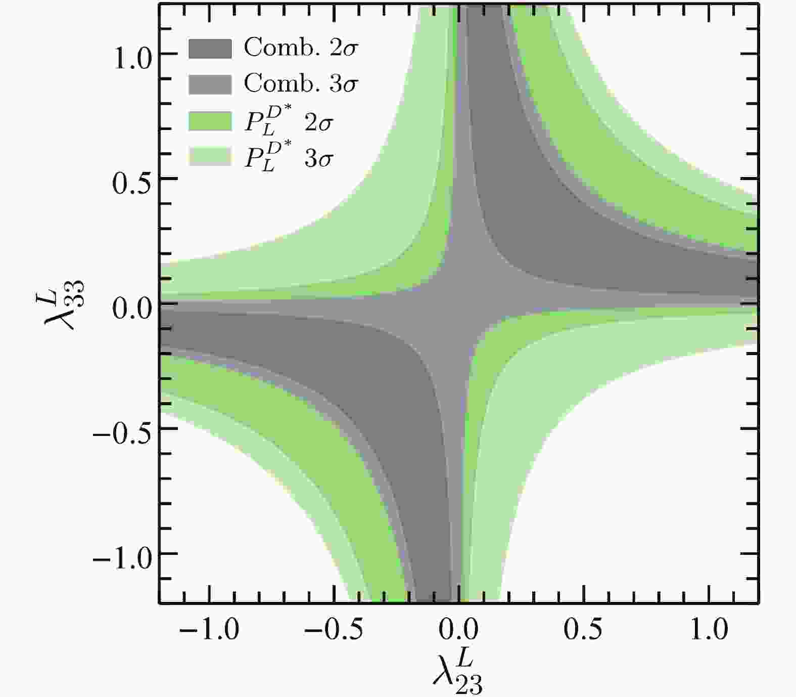
where a common LQ mass $M = 1{\,{\rm{TeV}}}$ is assumed. The solution with negative $\lambda_{23}^{L*}\lambda_{33}^L$ corresponds to the case in which the LQ interactions dominate over the SM contributions. We do not pursue this possibility in the following analysis. For the solution with positive $\lambda_{23}^{L*}\lambda_{33}^L$, the permitted regions of $(\lambda_{23}^L,\lambda_{33}^L)$ at both $2\sigma$ and $3\sigma$ levels are shown in Fig. 1. In this figure, we also show the individual constraint from the $D^*$ polarization fraction $P_L^{D^*}$, which remains weaker than the ones from $R_{D^{(*)}}$. In addition, the current measurement of the $\tau$ polarization fraction $P_L^\tau$ in $B\to D^* \tau \nu$ decay cannot provide any relevant constraint.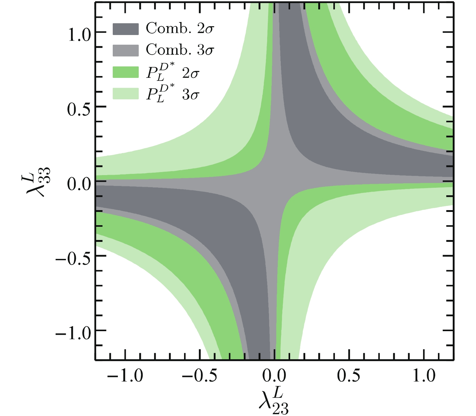

Figure 1.  (color online) Combined constraints on $(\lambda_{23}^L, \lambda_{33}^L)$ by all $b \to c \tau \bar\nu$ processes at $2\sigma$ (black) and $3\sigma$ (gray) levels. The dark (light) green area indicates the allowed region by $P_L^{D^*}$ only at $2\sigma$ ($3\sigma$).

As mentioned in Section 3, the LQ contributions to $b \to s \tau^+ \tau^-$ and $b \to c \tau \bar\nu_\tau$ depend on the same product $\lambda_{23}^{L*}\lambda_{33}^L$. In the case of positive $\lambda_{23}^{L*}\lambda_{33}^L$, we show in Fig. 2 the correlation between $R_{D^{(*)}}/R_{D^{(*)}}^{{\rm{SM}}}$ and ${\mathcal B} (B_s \to \tau^+ \tau^-)$. The LQ effects enhance the branching fraction of $B_s \to \tau^+ \tau^-$ in most of the parameter space. At present, the experimental upper limit $6.8 \times 10^{-3}$ [101] is far above the SM prediction $( 7.73 \pm 0.49) \times 10^{-7}$ [102]. However, to obtain the $2\sigma$ experimental range of $R_{D^{(*)}}$, the LQ contributions enhance ${\mathcal B} (B_s \to \tau^+ \tau^-)$ by about 2–3 orders of magnitude compared to the SM prediction, which reaches the expected LHCb sensitivity $5 \times 10^{-4}$ by the end of Upgrade II [55, 103]. The $B \to K^{(*)} \tau^+ \tau^-$ decay may also play an important role in probing the LQ effects. Although the Belle II experiment would improve the current upper limit $2.25 \times 10^{-3}$ at a 90% confidence level by no more than two orders of magnitude, the proposed FCC-ee collider can yield a few thousand of $B^0 \to K^{*0} \tau^+ \tau^-$ events from $\mathcal O (10^{13})$ Z decays [104].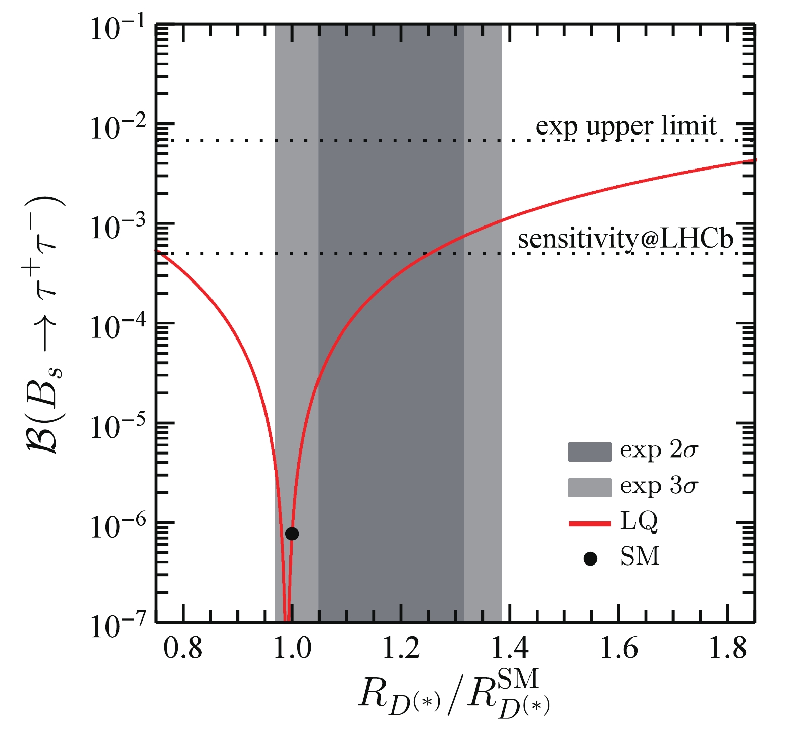

Figure 2.  (color online) Correlation between $R_{D^{(*)}}/R_{D^{(*)}}^{\rm SM}$ and ${\cal{B}}(B_s\to\tau^+ \tau^- )$. The black (gray) region denotes the $2\sigma$ ($3\sigma$) experimental ranges of $R_{D^{(*)}}/R_{D^{(*)}}^{\rm SM}$. The horizontal dashed and dotted lines correspond to the current LHCb upper limit and the expected sensitivity by the end of LHCb Upgrade II, respectively. The black point indicates the SM prediction.

Using the constrained parameter space at the $2\sigma$ level derived in the last subsection, we present predictions for the five $b \to c \tau \bar\nu$ processes. Table 2 shows the SM and LQ predictions for the branching fractions $\mathcal B$ and LFU ratios R of $B \to D^{(*)}\tau \bar\nu$, $B_c \to \eta_c \tau\bar\nu$, $B_c \to J/\psi \tau \bar\nu$, and $\Lambda_b \to \Lambda_c \tau\bar\nu$ decays. The LQ predictions include the uncertainties induced by the transition form factors and CKM matrix elements. Considering that the polarization fractions $P_L^\tau$ and $P_L^{D^*}$ have already been measured, their SM and LQ predictions are also shown in Table 2. Although the LQ predictions for the branching fractions ${\mathcal B}$ and the LFU ratios R of the $B_c \to \eta_c \tau \bar\nu$ and $B_c \to J/\psi \tau \bar\nu$ decays lie within the $1\sigma$ range of their respective SM values, they can be significantly enhanced by LQ effects.

We set out to analyze the $q^2$ distributions of the branching fraction $\mathcal B$, LFU ratio R, polarization fractions of the $\tau$ lepton ($P_L^\tau$), and daughter hadron ($P_{L,T}^{D^{*}}$, $P_{L,T}^{J/\psi}$, $P_L^{\Lambda_c}$), as well as the lepton forward-backward asymmetry $A_{\rm FB}$. The $B \to D \tau \nu$ and $B_c \to \eta_c \tau \bar\nu$ decays, both part of the "$B\to P$" transition, have differential observables in the SM and the LQ scenario as shown in Fig. 3. All differential observables of the $B \to D \tau \bar\nu$ and $B_c \to \eta_c \tau \bar\nu$ decays are similar to each other, while the observables in the latter have larger theoretical uncertainties due to the less precise $B_c \to \eta_c$ transition form factors. Therefore, the $B \to D \tau \bar\nu$ decay is more sensitive to the LQ effects, with the differential branching fraction largely enhanced, especially near $q^2 \sim 7{\,{\rm{GeV}}}^2$. The large difference between the SM and LQ predictions in this kinematic region could, therefore, provide a testable signature of the LQ effects. More interestingly, the $q^2$ distribution of the ratio R in the LQ model is enhanced in the entire kinematic region and does not have overlap with the $1\sigma$ SM range. In the future, more precise measurements of these distributions are of importance to confirm the existence of a possible NP effect in the $B \to D \tau \bar\nu$ decay. With regard to the forward-backward asymmetry $A_{{\rm{FB}}}$ and the $\tau$-lepton polarization fraction $P_L^\tau$ in both $B \to D \tau \bar\nu$ and $B_c \to \eta_c \tau\bar\nu$ decays, the LQ predictions are indistinguishable from the ones in SM, because the LQ effects only modify the Wilson coefficient ${\mathcal C}_L^{\ell \nu_\ell}$, which is canceled out exactly in the definitions of these observables (see Eqs. (16) and (17),Fig. 3). This feature is different from the NP scenarios that use scalar or tensor operators to explain the $R_{D^{(*)}}$ anomaly [58–60].

Figure 3.  (color online) $q^2$ distributions of observables in $B \to D \tau \bar\nu$ (left) and $B_c \to \eta_c \tau \bar\nu$ (right) decays. The black curves (gray band) indicate the SM (LQ) central values with $1\sigma$ theoretical uncertainty.

The $q^2$ distributions of the observables in $B \to D^* \tau \bar\nu$ and $B_c \to J/\psi \tau \bar\nu$ decays are shown in Fig. 4. Because both of these two decays belong to "$B \to V$" transition, their differential observables are similar. While the differential branching fractions of these two decays are enhanced in the LQ model, their theoretical uncertainties are larger than the ones in the $B \to D \tau \bar\nu$ decay. For the $q^2$ distributions of the ratios $R_{D^*}$ and $R_{J/\psi}$, they are largely enhanced in the entire kinematic region, especially in the large $q^2$ region. More importantly, although the ranges of the $q^2$-integrated ratio $R_{D^*,J/\psi}$ in the SM and the LQ scenario overlap at the $1\sigma$ level, the $1\sigma$ ranges of the differential ratio $R_{D^*,J/\psi}(q^2)$ at large $q^2$ in the SM and LQ exhiibt significant differences. The increases of $R_{D^*}$ and $R_{J/\psi}$ in the large $q^2$ region are larger than the one observed in $R_D$. Measurements of the differential ratios in the large dilepton invariant mass region are, therefore, crucial to confirm the $R_{D^{(*)}}$ anomaly and test the LQ model considered. Similarly to the ones in $B\to D \tau \bar\nu$ and $B_c \to \eta_c \tau \bar\nu$ decays, the angular distributions $A_{{\rm{FB}}}$, $P_{L,T}^{D^*,J/\psi}$, and $P_L^\tau$ are likewise not affected by the LQ effects, as shown in Fig. 4.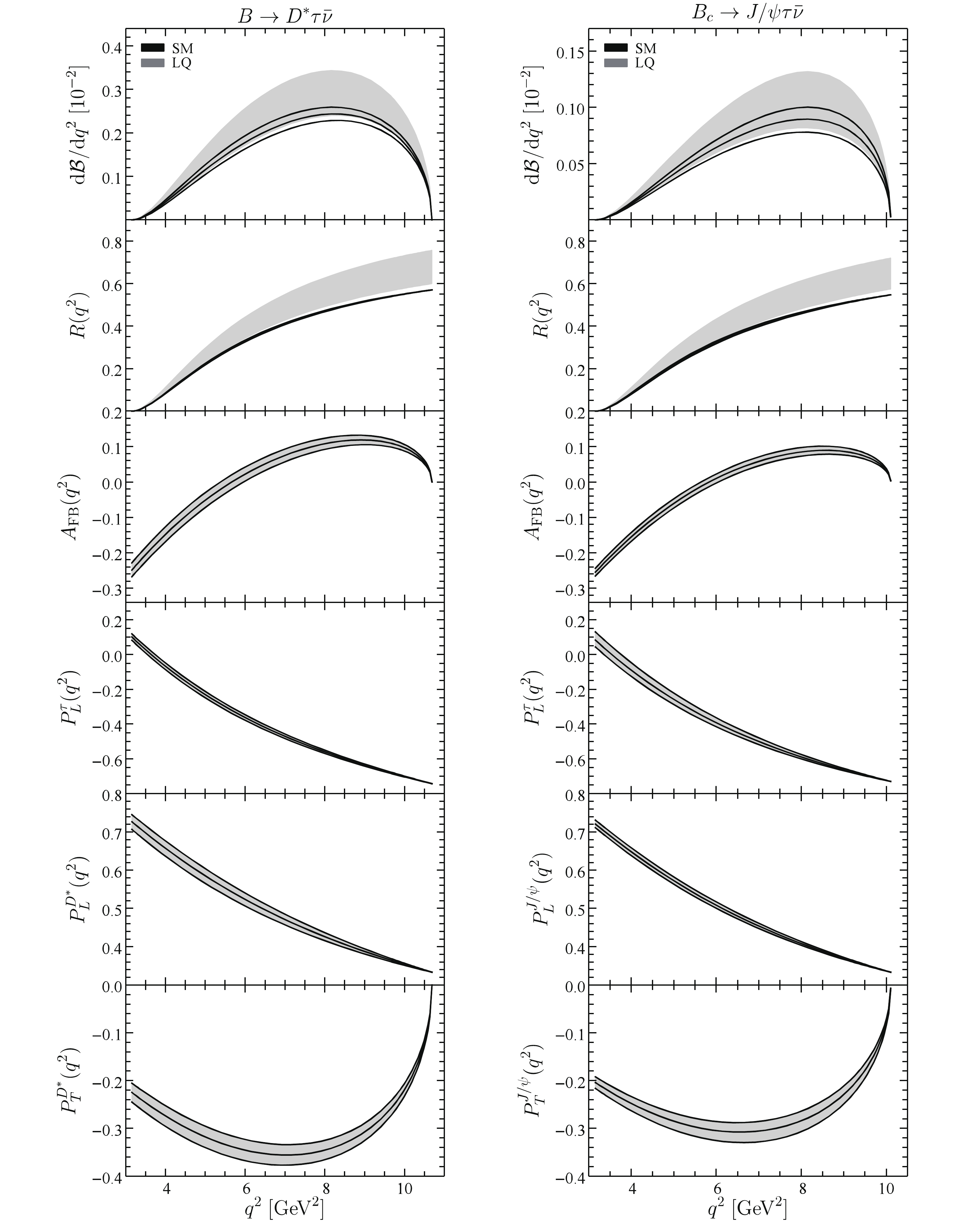

Figure 4.  (color online) $q^2$ distributions of observables in $B \to D^* \tau \bar\nu$ (left) and $B_c \to J/\psi \tau \bar\nu$ (right) decays. Other captions are the same as in Fig. 3.

For the $\Lambda_b \to \Lambda_c \tau \bar\nu$ decay, the $q^2$ distributions of the observables are shown in Fig. 5. The situation is similar in the $B \to D^* \tau \bar\nu$ and $B_c \to J/\psi \tau \bar\nu$ decays. The $q^2$ distributions of the branching fraction $\mathcal B$ and the ratio $R_{\Lambda_c}$ are greatly enhanced by the LQ effects. In the large $q^2$ region, the differential ratio $R_{\Lambda_c}$ exhibits a deviation between the $1\sigma$ permitted ranges of the SM and the LQ scenario. With the large numbers of $\Lambda_b$ obtained at the HL-LHC [78], we expect that this prediction could provide helpful information on the LQ effects. For the angular distributions, the LQ effects vanish due to the same reason as in the mesonic decays.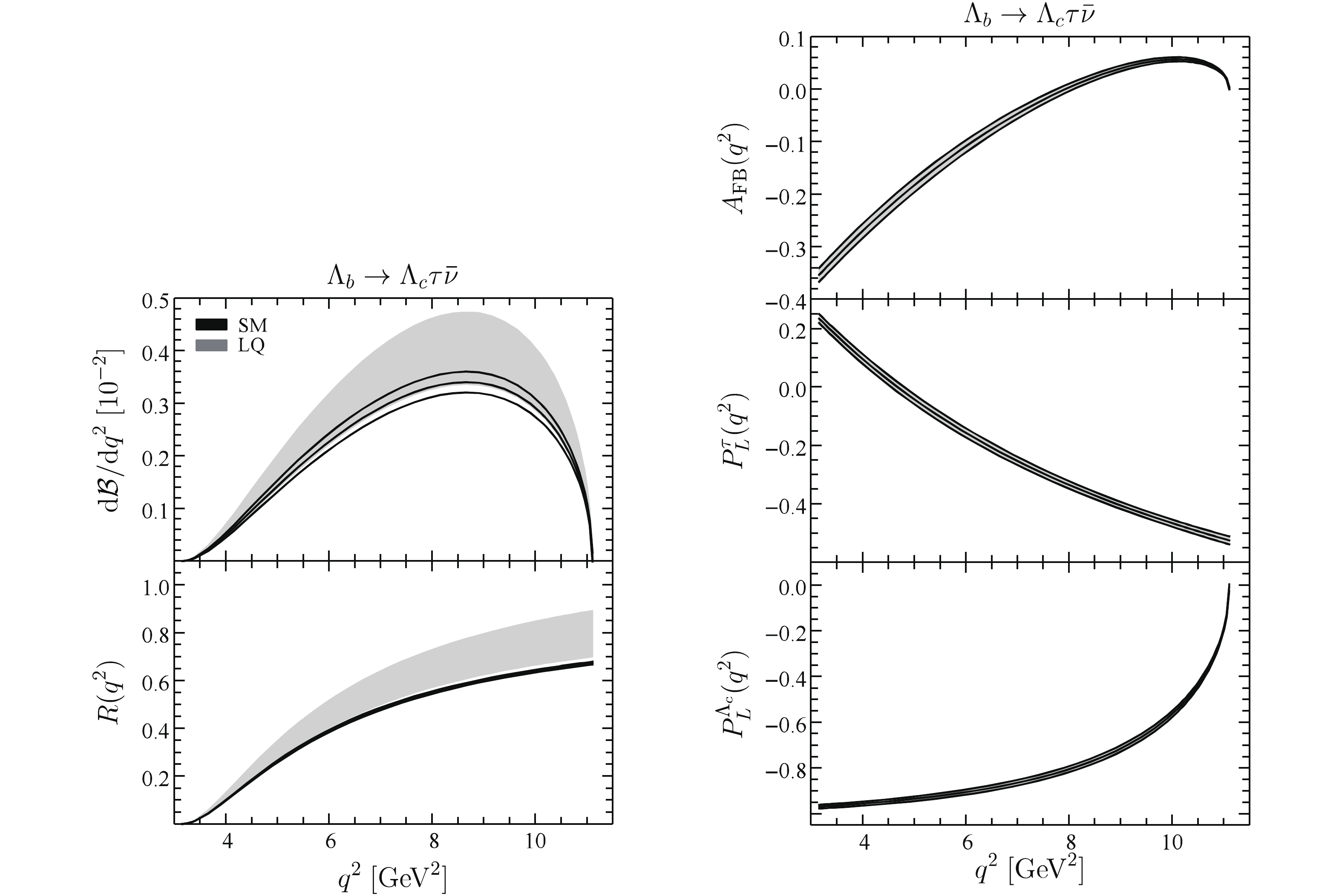

Figure 5.  (color online) $q^2$ distributions of observables in $\Lambda_b \to \Lambda_c \tau \bar\nu$ decay. Other captions are the same as in Fig. 3.

During the past few years, intriguing hints pointing towards an LFU violation have emerged in the $B \to D^{(*)} \tau \bar\nu$ data. Motivated by the recent measurements of $R_{J/\psi}$, $P_L^\tau$, and $P_L^{D^*}$, we revisited the LQ model proposed in Ref. [56], where two scalar LQs, one of which is a $SU(2)_L$ singlet, whereas the other is a $SU(2)_L$ triplet, are introduced simultaneously. Taking into account the recent progress on the transition form factors and the most recent experimental data, we obtained constraints on the LQ couplings $\lambda_{23}^L$ and $\lambda_{33}^L$. Subsequently, we systematically investigated the LQ effects on the five $b \to c \tau \bar\nu$ decays, $B \to D^{(*)}\tau \bar\nu$, $B_c \to \eta_c \tau\bar\nu$, $B_c \to J/\psi \tau \bar\nu$, and $\Lambda_b \to \Lambda_c \tau\bar\nu$. In particular, we focused on the $q^2$ distributions of the branching fractions, LFU ratios, and various angular observables. The main results of this study can be summarized as follows:

• After considering the $R_D$ and $R_{D^*}$ data, we obtain the bound on the LQ couplings, $0.03<\lambda_{23}^{L^*}\lambda_{33}^L<0.20$, at the $2\sigma$ level. The current measurements of $R_{J/\psi}$, $P_L^\tau$ and $P_L^{D^*}$ cannot provide further constraints on the LQ couplings.

• The $B_s \to \tau^+ \tau^-$ decay is strongly correlated with $B \to D^{(*)} \tau \bar\nu$. To reproduce the $2\sigma$ experimental range of $R_{D^{(*)}}$, the LQ effects enhance ${\mathcal B}(B_s \to \tau^+ \tau^-)$ by about 2–3 orders of magnitude compared to the SM prediction and hence reach the expected sensitivity of the LHCb Upgrade II.

• The differential branching fractions and LFU ratios are largely enhanced by the LQ effects. Due to their small theoretical uncertainties, the latter provide testable signatures of the LQ model considered, especially in the large dilepton invariant mass squared region. Moreover, $R_{\Lambda_c}$ in the baryonic decay $\Lambda_b \to \Lambda_c \tau \bar\nu$ has the potential to shed new light on the $R_{D^{(*)}}$ anomalies.

• Because no new operators are generated by the LQ effects, all angular distributions in the LQ model are the same as in the SM. We provide the most recent SM predictions for the $\tau$-lepton forward-backward asymmetry, the $\tau$, and meson polarization fractions of the five $b \to c \tau \bar\nu$ modes. Although precision measurements of these angular distributions are very challenging at the HL-LHC and SuperKEKB, they are crucial for the verification of the LQ scenario investigated in this work.

The $q^2$ distributions of the branching fractions, the LFU ratios, and the various angular observables in $b \to c \tau \bar\nu$ transitions can help to confirm possible NP resolutions of the $R_{D^{(*)}}$ anomalies and distinguish among the various NP candidates. With the experimental progress expected from the SuperKEKB [54] and the future HL-LHC [78], our predictions for these observables can be further probed in the near future.

Note Added. After the completion of this work, the Belle Collaboration announced their results of $R_{D}$ and $R_{D^*}$ with a semileptonic tagging method [105,106]. The measured values are $R_D^{\rm exp} = 0.307\pm 0.037\,({\rm stat.})\pm 0.016\,({\rm syst.})$ and $R_{D^*}^{\rm exp} = 0.283\pm 0.018 \, ({\rm stat.})\pm 0.014 \,({\rm syst.})$. After including this new measurement, the world averages become $R_D^{\rm avg,\,2019} = 0.337\pm 0.030$ and $R_{D^*}^{\rm avg,\,2019} = 0.299\pm 0.013$ [107]. The deviation of the current world averages from the SM predictions decreases from $3.8\sigma$ to $3.1\sigma$ [105]. Because the difference between the new and previous averages is small, our numerical results are expected to remain qualitatively unchanged. For example, the updated bounds on $\lambda_{23}^{L*}\lambda_{33}^L$ in Eq. (23) becomes $-2.88<\lambda _{23}^{L*}\lambda _{33}^L <-2.73$ and $0.02<\lambda _{23}^{L*}\lambda _{33}^L<0.17$.

We thank Xin-Qiang Li for useful discussions.

In the presence of NP, the most general effective Hamiltonian for the $b\to c\tau\bar{\nu}$ transition can be written as [23, 76]

In this appendix, for completeness, we consider the most general case of NP and provide the helicity amplitudes in the five $b \to c \tau \bar\nu$ decays, $B \to D^{(*)}\tau \bar\nu$, $B_c \to \eta_c \tau\bar\nu$, $B_c \to J/\psi \tau \bar\nu$, and $\Lambda_b \to \Lambda_c \tau\bar\nu$. Explicit expressions of the spinors and polarization vectors used to calculate the helicity amplitudes are also presented.

To calculate the hadronic helicity amplitudes of $M\to N\tau \bar\nu$ in Eq. (13), we work in the M rest frame and follow the notation of Ref. [79]:

where $q^{\mu}$ is the four-momentum of the virtual vector boson in the M rest frame, and

Subsequently, substituting the momentum into Eq. (A12), the Dirac spinors in the $\Lambda_b\to\Lambda_c\tau\nu_{\tau}$ decay can be written as

where $\chi(\vec{p}_{\Lambda_b},1/2) = \chi(\vec{p}_{\Lambda_c},1/2) = (1,0)^T,\chi(\vec{p}_{\Lambda_b},-1/2) = \chi(\vec{p}_{\Lambda_c}, -1/2) =$$(0,1)^T.$.

In the $B \to D^* \tau \bar\nu$ decay, the polarization vectors of the $D^*$ meson are given by

In all the five $b \to c \tau \bar\nu$ decays, the polarization vectors for the virtual vector boson W can be written as

and the orthonormality and completeness relation [108]

where $g_{mn} = {\rm diag}(+1,-1,-1,-1)$.

In the calculation of the leptonic helicity amplitudes, we work in the rest frame of the virtual vector boson W, which is equivalent to the rest frame of the $\tau$-$\bar{\nu}_\tau$ system. Following Ref. [79], we have

where $|\vec{p}_\tau| = \sqrt{q^2} v^2/2$, $E_\tau = |\vec{p}_\tau| + m_\tau^2/\sqrt{q^2}$, $v = \sqrt{1-m_\tau^2/q^2}$, and $\theta_\tau$ denotes the angle between the three-momenta of the $\tau$ and the N.

The Dirac spinors for $\tau$ and $\bar\nu_\tau$ read

respectively. Further details are given in Appendix A.2

The polarization vectors of the virtual vector boson in the W rest frame are written as

which can also be obtained from Eq. (A6) by a Lorentz transformation and satisfy the orthonormality and completeness relation in Eq. (A7).

The definitions of the helicity operator $h_{\vec{p}}$ and its eigenstates are given as follows [109]

where $\vec{p}$ denotes the momentum of the particle, and $\vec{\sigma} = \{\sigma^1,\sigma^2,\sigma^3\}$ are the Pauli matrices. Eigenstates of the helicity operator $h_{\vec{p}}$ read

for the normalized momentum $\hat{\vec{p}} = \{\sin\theta\cos\phi,\sin\theta\sin\phi,\cos\theta\}$.

Using these eigenstates, the solution of Dirac equation $(\gamma^{\mu} p_{\mu}-m)u(\vec{p},s) = 0$ in Dirac representation can be written as

Further, the spinor for the antiparticle can be obtained by $v(\vec{p},s)\equiv C\bar{u}(\vec{p},s)^{T} = i\gamma^0\gamma^2 \bar{u}(\vec{p},s)^{T}$^②, whose explicit expression reads

where $\xi(\vec{p},s) = \chi(\vec{p},-s)$ and $\xi(\vec{p},s)$ satisfies $h_{\vec{p}}\; \xi(\vec{p},s) = -s\; \xi(\vec{p},s)$.

The spinors in Weyl representation read

They can also be obtained from the Dirac representation by the relation $u_{W}(\vec{p},s) = X u(\vec{p},s)$ with the transformation matrix

In the $\tau$-$\bar\nu_\tau$ center-of-mass frame, we emphasize that if the $\tau$ spinor is specified as $u(\vec{p},s)$ in the leptonic helicity amplitude, then the $\bar\nu_\tau$ spinor has the form $v(-\vec{p},s)$, as in Eq. (A9). All calculations in our work are depictec in Dirac representation.

The leptonic helicity amplitudes in Eq. (13) are defined as [79]

Obtaining $L^T_{\lambda_\tau,\lambda_{W_1} ,\lambda_{W_2}} = -L^T_{\lambda_\tau ,\lambda_{W_2},\lambda_{W_1}}$is straightforward. The non-zero leptonic helicity amplitudes read

The hadronic helicity amplitudes $M \to N$ are defined as

and

$H^{T,\lambda_M}_{\lambda_N,\lambda_{W_1} ,\lambda_{W_2}} = -H^{T,\lambda_M}_{\lambda_N,\lambda_{W_2} ,\lambda_{W_1}}$is easily obtained. The amplitudes $H_{\lambda_N,\lambda_{W_1},\lambda_{W_2}}^{T_1,\lambda_M}$ and $H_{\lambda_N,\lambda_{W_1},\lambda_{W_2}}^{T_2,\lambda_M}$ are connected by the relation $\sigma_{\mu \nu}\gamma_{5} = -(i/2)\epsilon^{\mu\nu\alpha\beta}\sigma_{\alpha\beta}$, where $\epsilon^{0123} = -1$.

The hadronic matrix elements for the $B\to D$ transition can be parameterized in terms of form factors $F_{+,0,T}$ [110, 111]. In the BGL parametrization, the form factors $F_{+,0}$ can be written as expressions of $a_n^+$ and $a_n^0$ [13],

where $r = m_D / m_B$, ${\cal N} = (1+r)/(2\sqrt{r})$, $w = (m_{B}^2+m_{D}^2-q^{2})/(2m_{B}m_{D})$, $z(w,{\cal N}) = (\sqrt{1+w}-\sqrt{2{\cal N}})/(\sqrt{1+w}+\sqrt{2{\cal N}})$, and $F_+(0) = F_0(0)$. The values of the fit parameters are taken from Ref. [13]. Expressions of the tensor form factor $F_T$ can be found in Ref. [110].

For $B\to D^*$ transition, the relevant form factors $\{V,A_{0,1,2}\}$ can be written in terms of the form factors $\{h_V,h_{A_{1,2,3}}\}$ in the heavy quark effective theory (HQET) [110],

where $m_\pm = m_B \pm m_{D^*}$ and $w = (m_B^2+m_{D^*}^2-q^2)/2m_Bm_{D^*}$. In the CLN parametrization, the HQET form factors can be expressed as [89]

with $r = m_{D^*}/m_B$. Numerically we obtain,

with $z = (\sqrt{w+1}-\sqrt{2})/(\sqrt{w+1}+\sqrt{2})$. The fit parameters $R_{1}(1)$, $R_{2}(1)$, $h_{A_1}(1)$ and $\rho_{D^{*}}^2$ are taken from Ref. [14]. Expressions of the tensor form factors $T_{1,2,3}$ can be found in Ref. [110].

The $\Lambda_b\rightarrow\Lambda_c$ hadronic matrix elements can be written in terms of ten helicity form factors $\{F_{0,+,\perp},G_{0,+,\perp},h_{+,\perp},\widetilde{h}_{+,\perp}\}$ [75, 76]. Following Ref. [75], the lattice calculations are fitted to two (Bourrely-Caprini-Lellouch) BCL z-parametrizations. In the so called "nominal" fit, a form factor f reduces to the form

while a form factor f in the higher-order fit is given by

where $t_0 = (m_{\Lambda_b} - m_{\Lambda_c})^2$, $t_+^f = (m_{\rm pole}^f)^2$, and $z^f(q^2) = \left.\left(\sqrt{t_+^f-q^2}-\sqrt{t_+^f-t_0}\right)\right/$$\left(\sqrt{t_+^f-q^2}+\sqrt{t_+^f-t_0}\right)$.The values of the fit parameters and all the pole masses are taken from Ref. [76].

In addition, the form factors for $B_c \to J/\psi\ell\bar{\nu_\ell}$ and $B_c \to \eta_c\ell\bar{\nu_\ell}$ decays are taken form the results in the Covariant Light-Front Approach in Ref. [18].

Because similar expressions hold for the $B \to D \tau \bar\nu$ and $B_c \to \eta_c \tau \bar\nu$ decays, we only provide the theoretical formulae of the former. Using the form factors in Appendix B, the non-zero helicity amplitudes for the $B \to D \tau \bar\nu$ decay in Eq. (A18) can be written as

Subsequently, the differential decay width in Eq. (11) and angular observables in Eq. (16) and (17) are obtained

with

Because similar expressions hold for the $B \to D^* \tau \bar\nu$ and $B_c \to J/\psi \tau \bar\nu$ decays, only theoretical formulae of the former are provided in this subsection. Using the form factors in Appendix B, the non-zero helicity amplitudes for the $B \to D^* \tau \bar\nu$ decay in Eq. (A18) can be written as

with $m_\pm = m_B \pm m_{D^*}$. Then, the differential decay width in Eq. (11) and the angular observables in Eq. (16) and (17) are obtained, respectively, as

with

Using the transition form factors in Appendix B, the helicity amplitudes for the $\Lambda_b \to \Lambda_c$ decay in Eq. (A18) can be written as

with $m_\pm = m_{\Lambda_b}\pm m_{\Lambda_c}$. Thus, the differential decay width in Eq. (11) can be written as

with

where $\sum$ depicts the summation over $s = \pm 1/2$. For the forward-backward asymmetry in Eq. (16), we obtain

where

For the $\Lambda_c$ longitudinal polarization fraction in Eq. (17), we obtain

where

For the $\tau$-lepton longitudinal polarization fraction, we obtain

where