


 Abstract
 HTML
HTML Reference
 Related
 PDF
PDF


-
The current cosmic acceleration is an unexpected picture of the universe, revealed by the data sets of the last two decades from astrophysics and cosmology [1-15]. These data, which come from the cosmic microwave background radiation, supernovae surveys, baryon acoustic oscillations, etc, indicate that the universe consists of 5% ordinary baryonic matter, 27% dark matter, and 68% dark energy [6-16]. Dark energy not only has an unknown form of energy but also has not been detected directly. Additionally, dark energy is very similar to the cosmological constant which was proposed by Einstein. In Planck units, the observed value of the cosmological constant is an extravagantly tiny positive value of order
$ 10^{-124} $ . This is the well-known cosmological constant fine tuning problem [17, 18]. There have been numerous attempts in order to solve this problem, such as quintessence, the anthropic principle, the$ f(R) $ model, etc. [19-26]. But none of these theories are problem-free. In astrophysics and cosmology, it is still an open question.Another perspective for resolving the problem described above, which seems to be more radical, is the following: must the dimensions of our universe be four? Are there any extra dimensions which are too small to be observed? Does the evolution of these extra dimensions contribute to the current cosmic acceleration? If so, would this help in solving the cosmological constant fine tuning problem? Therefore, we have investigated some higher-dimensional theories [27-40]. Among them, the Randall-Sundrum (RS) two-brane model [30], which has a natural solution to the hierarchy problem with warped extra dimension, has attracted our attention. The hierarchy problem is essentially a fine tuning problem that can be described as: why is there such a large discrepancy between the electroweak scale/Higgs mass
$ M_{EW}\sim1 $ TeV and the Planck mass$ M_{pl}\sim10^{16} $ TeV? In the RS two-brane scenario, our universe is described by a five dimensional line element [30]$ {\rm d}s^{2} = {\rm e}^{-2\sigma(y)}\eta_{\mu\nu}{\rm d}x^{\mu}{\rm d}x^{\nu}+r_{c}^{2}{\rm d}y^{2}, $

(1) where y is the extra dimensional coordinate,
$ r_{c} $ is the extra dimensional compactification radius,$ {\rm e}^{-2\sigma} $ is the well-known warp factor with the term$ \sigma = kr_{c}|\phi| $ ,$ k = \sqrt{-\Lambda/24M^{3}} $ , and M is the five dimensional Planck mass. Then a large hierarchy is generated by the warp factor$ {\rm e}^{-2kr_{c}\pi} $ , meanwhile one requires only$ kr\approx10 $ . The cosmological constant fine tuning problem is similar to the hierarchy problem. In the RS model, the visible brane is unstable, which is caused by the negative brane tension. Furthermore, the cosmological constant on the visible brane is zero, which is not consistent with our data sets of the last two decades [31, 41].The above problems can be solved in a generalized RS braneworld scenario in which
$ g_{\mu\nu} $ replaces$ \eta_{\mu\nu} $ in the RS model [31]. In this scenario, the tension of the visible brane and the hidden brane can both be positive with a negative induced cosmological constant. It is very interesting because both branes are stable [42-47]. In order to be consistent with the current constraints, the negative induced cosmological constant$ \Omega $ should be transformed into the positive effective cosmological constant$\Omega_{\rm eff}$ . This positive$\Omega_{\rm eff}$ can be obtained in an$ (n+1) $ -dimensional (-d) generalized RS model with two$ (n-1) $ -branes instead of two 3-branes [48]. In this model, adopting an anisotropic metric ansatz with two different scale factors, one obtains the positive effective cosmological constant$\Omega_{\rm eff}\sim10^{-124}$ (in Planck units), which only needs a solution$ kr\simeq50-80 $ without fine tuning. The cosmological constant fine tuning problem can be solved quite well [48].But there is no reason to exclude the possibility of the anisotropic metric ansatz with the form of scale factors more than two. In this paper, we investigate an
$ (n+1) $ -dimensional generalized Randall-Sundrum model with an anisotropic metric that has three different scale factors. We obtain that$ H_{1} $ has a lower bound,$H_{\rm 1min}$ . Near this minimum value, the Hubble parameter is seen to be a constant in a large region, thus causing the acceleration of the universe. Meanwhile, the scale of extra dimension is smaller than the observed scale but greater than the Planck length. This may suggest that the observed present acceleration of the universe is caused by the extra-dimensional evolution rather than by dark energy. Our work is organized as follows: In Sec. 2, by considering the two$ (n-1) $ -branes with the matter field Lagrangian in the$ (n+1) $ -d generalized RS model, the n-d Einstein field equations are obtained. In Sec. 3, we focus on the evolution of a$ (n+1) $ -brane solved from the above field equation with an anisotropic metric ansatz that has three different scale factors. Finally, the summary and conclusion are presented in Sec. 4. -
We consider an
$ (n+1) $ -d generalized RS braneworld model that is consistent with Ref. [48]. The action$ S_{n+1} $ is:$ S_{n+1} = S_{\rm bulk}+S_{\rm vis}+S_{\rm hid} , $

(2) where
$S_{\rm bulk}$ is the bulk action and$S_{\rm vis}$ and$S_{\rm hid}$ are the$ (n-1) $ -brane visible action and hidden action, respectively:$ S_{\rm bulk} = \int {\rm d}^{n}x{\rm d}y\sqrt{-G}(M^{n-1}_{n+1}R-\Lambda) , $

(3) $ S_{\rm vis} = \int {\rm d}^{n}x\sqrt{-g_{\rm vis}}({\cal{L}}_{\rm vis}-V_{\rm vis}), $

(4) $ S_{\rm hid} = \int {\rm d}^{n}x\sqrt{-g_{\rm hid}}({\cal{L}}_{\rm hid}-V_{\rm hid}), $

(5) where
$ \Lambda $ denotes a bulk cosmological constant,$ M_{n+1} $ is the$ (n+1) $ -d fundamental mass scale,$ G_{AB} $ and R are the$ (n+1) $ -d metric tensor and Ricci scalar, respectively,$ {\cal{L}}_{i} $ is the matter field Lagrangian of the visible and hidden branes, and$ V_{i} $ is the tension of the visible and hidden branes, here with$i = {\rm hid}$ or${\rm vis}$ . In this$ (n+1) $ -d generalized RS scenario, the metric takes the form:$ {\rm d}s^{2} = G_{AB}{\rm d}x^{A}{\rm d}x^{B} = {\rm e}^{-2A(y)}g_{ab}{\rm d}x^{a}{\rm d}x^{b}+r^{2}{\rm d}y^{2}, $

(6) where
$ {\rm e}^{-2A(y)} $ is known as the warp factor, capital letter$ A,B,... $ indices run over all spacetime coordinate labels, y is the extra dimensional coordinate of length r, lowercase letter$ a,b = 0,1,2,\cdot\cdot\cdot,n-1 $ does not include the coordinate y, and$ g_{ab} $ is the n-d metric tensor. Variation with respect to the metric$ G_{AB} $ and after some easy manipulations then modulo surface terms, one obtains$ \begin{split} R_{AB}-\frac{1}{2}G_{AB}R =& \frac{1}{2M^{n-1}_{n+1}}\bigg\{-G_{AB}\Lambda+\sum\limits_{i}\big[T^{i}_{AB} \delta(y-y_{i}) \\ & -G_{ab}\delta_{A}^{a}\delta_{B}^{b}V_{i}\delta(y-y_{i})\big]\bigg\}, \end{split} $

(7) where
$ R_{AB} $ is the$ (n+1) $ -d Ricci tensor and$ T^{i}_{AB} $ is the$ (n+1) $ -d energy-momentum tensors. Note that here the energy-momentum tensor is given by$T^{ia}_{b} = {\rm diag}[-c_{i},c_{i},\cdot\cdot\cdot,c_{i}]$ [47, 48]. A solution to Eq. (7) with the metric tensor in Eq. (6) has been derived in Ref. [48], and reads$ A = -\ln[\omega\cosh(k|y|+c_{-})], $

(8) where the constant
$ k\equiv\sqrt{-\Lambda/[M^{n-1}_{n+1}n(n-1)]}\simeq $ Planck mass.$ \omega $ is given by$ \omega\equiv\sqrt{\frac{-2\Omega}{(n-1)(n-2)k^{2}}}, $

(9) and the term
$ c_{-} $ takes the form$ c_{-}\equiv\ln\frac{1-\sqrt{1-\omega^{2}}}{\omega}. $

(10) Meanwhile, an n-d Einstein field equation can be obtained:
$ \ \widetilde{R}_{ab}-\frac{1}{2}g_{ab}\widetilde{R} = -\Omega g_{ab}, $

(11) where
$ \Omega $ is the induced cosmological constant on the visible brane, and$ \widetilde{R} $ and$ \widetilde{R}_{ab} $ are the n-d Ricci scalar and Ricci tensor, respectively,Note that the solution derived above has the negative induced cosmological constant
$ \Omega $ . Here we do not consider the situation where$ \Omega>0 $ , since the tension on the visible brane is negative, which results in instability [31, 41, 47, 48]. Thus, an anisotropic metric is assumed to be of the following form [47-49]:$ g_{ab} = {\rm diag}[-1,a_{1}^{2}(t),a_{2}^{2}(t),a_{3}^{2}(t),\cdot\cdot\cdot,a_{n-1}^{2}(t)], $

(12) where
$ a_{i} $ is the scale factor. The case where the scale factors on the visible brane evolve with two different rates has been studied recently [48]. In this case, we can obtain the positive effective cosmological constant$\Omega_{\rm eff}\simeq{10}^{-124}$ and only requiring$ kr\simeq50-80 $ , where for convenience, the Planck mass has been set to unity. Thus, the cosmological constant fine tuning problem can be solved quite well. Furthermore, the three dimensional (3D) Hubble parameter$ H(z) $ is consistent with the cosmic chronometers dataset extracted from [6-15]. The observed 3D universe naturally shifts from deceleration expansion to accelerated expansion. This shows that the accelerated expansion of the observed universe is intrinsically an extra-dimensional phenomenon. But there is no reason to make the scale factor evolve with only two kinds of rates. Therefore, we investigate the case where the scale factors on the visible brane evolve with three different rates. -
For the anisotropic metric Eq. (12) with three kinds of scale factors and the negative induced cosmological constant
$ \Omega\sim-10^{-124} $ , the field equations (11) can be written:$ \sum\limits_{i}n_{i}(n_{i}-1)H_{i}^{2}+\sum\limits_{i\neq j}n_{i}n_{j}H_{i}H_{j} = 2\Omega, $

(13) $ \sum\limits_{i}n_{i}\dot{H}_{i}-\dot{H}_{1}+\left(\sum\limits_{i}n_{i}H_{i}\right)^{2}-H_{1}\sum\limits_{i}n_{i}H_{i} = 2\Omega, $

(14) $ \sum\limits_{i}n_{i}\dot{H}_{i}-\dot{H}_{2}+\left(\sum\limits_{i}n_{i}H_{i}\right)^{2}-H_{2}\sum\limits_{i}n_{i}H_{i} = 2\Omega, $

(15) $ \sum\limits_{i}n_{i}\dot{H}_{i}-\dot{H}_{3}+\left(\sum\limits_{i}n_{i}H_{i}\right)^{2}-H_{3}\sum\limits_{i}n_{i}H_{i} = 2\Omega, $

(16) where
$ i = 1,2,3 $ , and the terms$ n_{1} $ ,$ n_{2} $ , and$ n_{3} $ are the number of dimensions which evolve with three kinds of rates, respectively, the Hubble parameter$ H\equiv\dot{a}/a $ , and$ \dot{H}_{i} $ is the first time derivative of$ {H}_{i} $ . Computing the sum of Eqs. (14), (15), and (16) yields a simplified expression for$ \displaystyle\sum_{i}n_{i}H_{i} $ :$ \sum\limits_{i}n_{i}H_{i} = -\chi_{1}\tan\beta, $

(17) where the term
$ \beta = \chi_{1}t+\theta_{0} $ ,$ \theta_{0} $ is the initial phase angle which is determined by the scale of the formation of the brane, and the term$ \chi_{1} $ takes the form$ \chi_{1} = \sqrt{\frac{-2(n-1)\Omega}{n-2}}. $

(18) It is convenient to redefine the sum of the Hubble parameters in the following manner:
$ \sum\limits_{i}n_{i}H_{i}\equiv f. $

(19) Replacing Eqs. (17) and (19) into Eq. (14), then performing some manipulations, one obtains
$ \dot{H}_{1}+H_{1}f = \dot{f}+f^{2}-2\Omega. $

(20) The solution of the above equation is
$ H_{1} = {\rm e}^{-\int f{\rm d}t}\left[\int(\dot{f}+f^{2}-2\Omega){\rm e}^{\int f{\rm d}t}{\rm d}t +c\right] , $

(21) where c is an integration constant. Combining Eqs. (17) and (19),
$ H_{1} $ is given by$ H_{1} = -\frac{\chi_{1}}{n-1}\tan\beta+c\sec\beta . $

(22) Using Eqs. (19) and (20), Eq. (13) can be rewritten as
$ n_{2}H_{2}^{2}+n_{3}H_{3}^{2} = -n_{1}H_{1}^{2}+f^{2}-2\Omega. $

(23) Eqs. (22) and (23) could be combined to give the following equation, eliminating
$ H_{2} $ completely:$ \begin{split} & \left(n_{3}+\frac{n_{3}^{2}}{n_{2}}\right)H_{3}^{2}+\frac{2n_{3}}{n_{2}}(n_{1}H_{1}-f)H_{3}+\Bigg[\left(\frac{1}{n_{2}}-1\right)f^2 \\ & \quad +\frac{n_{1}^{2}}{n_{2}}H_{1}^{2}-\frac{2n_{1}}{n_{2}}fH_{1}+n_{1}H_{1}^{2}+2\Omega\Bigg] = 0. \end{split} $

(24) Then the Hubble parameter
$ H_{3} $ can be obtained:$ \begin{split} H_{3} =& \frac{f-n_{1}H_{1}}{n_{2}+n_{3}}-\frac{1}{n_{2}+n_{3}}\Bigg[\frac{n_{2}}{n_{3}}(n_{2}+n_{3}-1)f^{2} \\ & -\frac{n_{1}n_{2}}{n_{3}}(n-1)H_{1}^{2}+\frac{2n_{1}n_{2}}{n_{3}}fH_{1} \\ & -\frac{2n_{2}}{n_{3}}(n_{2}+n_{3})\Omega\Bigg]^{1/2} . \end{split} $

(25) Combining Eqs. (17), (19), and (22),
$ H_{3} $ is given by$ H_{3} = -\frac{\chi_{1}}{n-1}\tan\beta-\frac{\chi_{3}+n_{1}c}{n_{2}+n_{3}}\sec\beta , $

(26) where the term
$ \chi_{3} $ is$ \chi_{3} = \sqrt{-2\frac{n_{2}}{n_{3}}(n_{2}+n_{3})\Omega-n_{1}\frac{n_{2}}{n_{3}}(n-1)c^{2}}. $

(27) Note here that we have chosen
$ H_{2} $ to always be greater than$ H_{3} $ . Finally, using Eqs. (17) and (26), one can also obtain the Hubble parameter$ H_{2} :$ $ H_{2} = -\frac{\chi_{1}}{n-1}\tan\beta+\frac{\chi_{2}-n_{1}c}{n_{2}+n_{3}}\sec\beta , $

(28) where the term
$ \chi_{2} $ is$ \chi_{2} = \sqrt{-2\frac{n_{3}}{n_{2}}(n_{2}+n_{3})\Omega-n_{1}\frac{n_{3}}{n_{2}}(n-1)c^{2}} . $

(29) It is easy to see that the integration constant c is constrained by Eqs. (27) and (29). The constant c must be set to a value less than
$c_{\rm max}$ to guarantee that the value in the root is greater than zero, which yields$ c\leqslant\sqrt{\frac{-2\Omega(n_{2}+n_{3})}{n_{1}(n-1)}}\equiv c_{\rm max}, $

(30) where
$c_{\rm max}$ is the maximum value of c. It is evident from Eqs. (26), (27), (28), and (29) that, if$c = c_{\rm max}$ ,$ H_{2} $ is equal to$ H_{3} $ . For convenience, we define a parameter d satisfying$ c = dc_{\rm max}, $

(31) where the value of d is between 0 and 1. First, we investigate the effect of parameter d on the Hubble parameters H. We choose
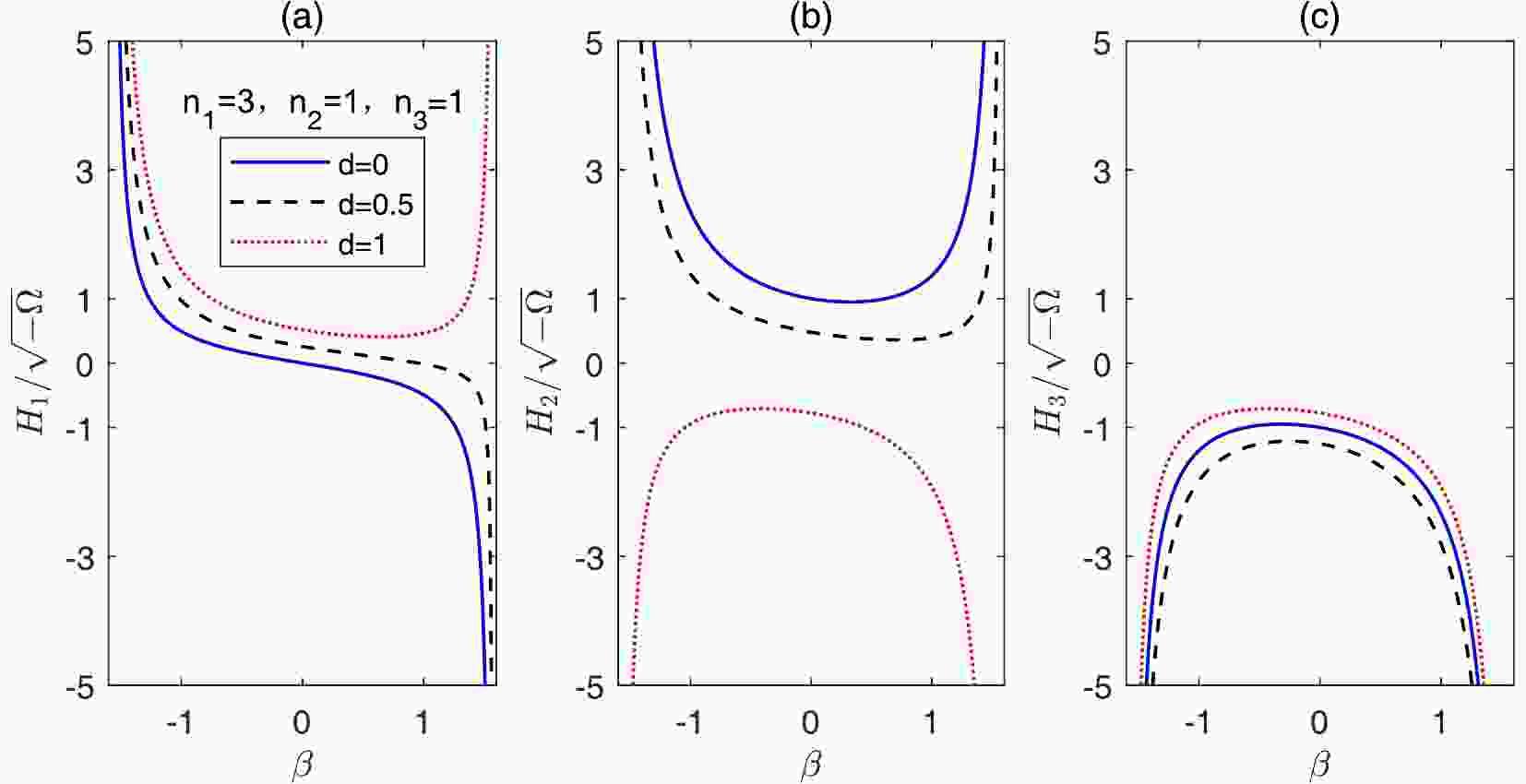
$ n_{1} = 3 $ , which is most in line with the presently observed three dimensional (3D) space. Further setting$ n_{2} = 1 $ and$ n_{3} = 1 $ , we plot the Hubble parameters$ H_{1} $ ,$ H_{2} $ , and$ H_{3} $ as a function of$ \beta $ in Fig. 1 with$ d = 0 $ ,$ d = 0.5 $ , and$ d = 1 $ respectively. In Fig. 1(a)-(c), the three curves having same type (color) correspond to three different values of d, respectively. In Fig. 1(a), we plot the Hubble parameter$ H_{1} $ as a function of$ \beta $ . When the parameter is$ d = 0 $ or$ d = 0.5 $ , the Hubble parameter$ H_{1} $ monotonically decreases with$ \beta $ . And when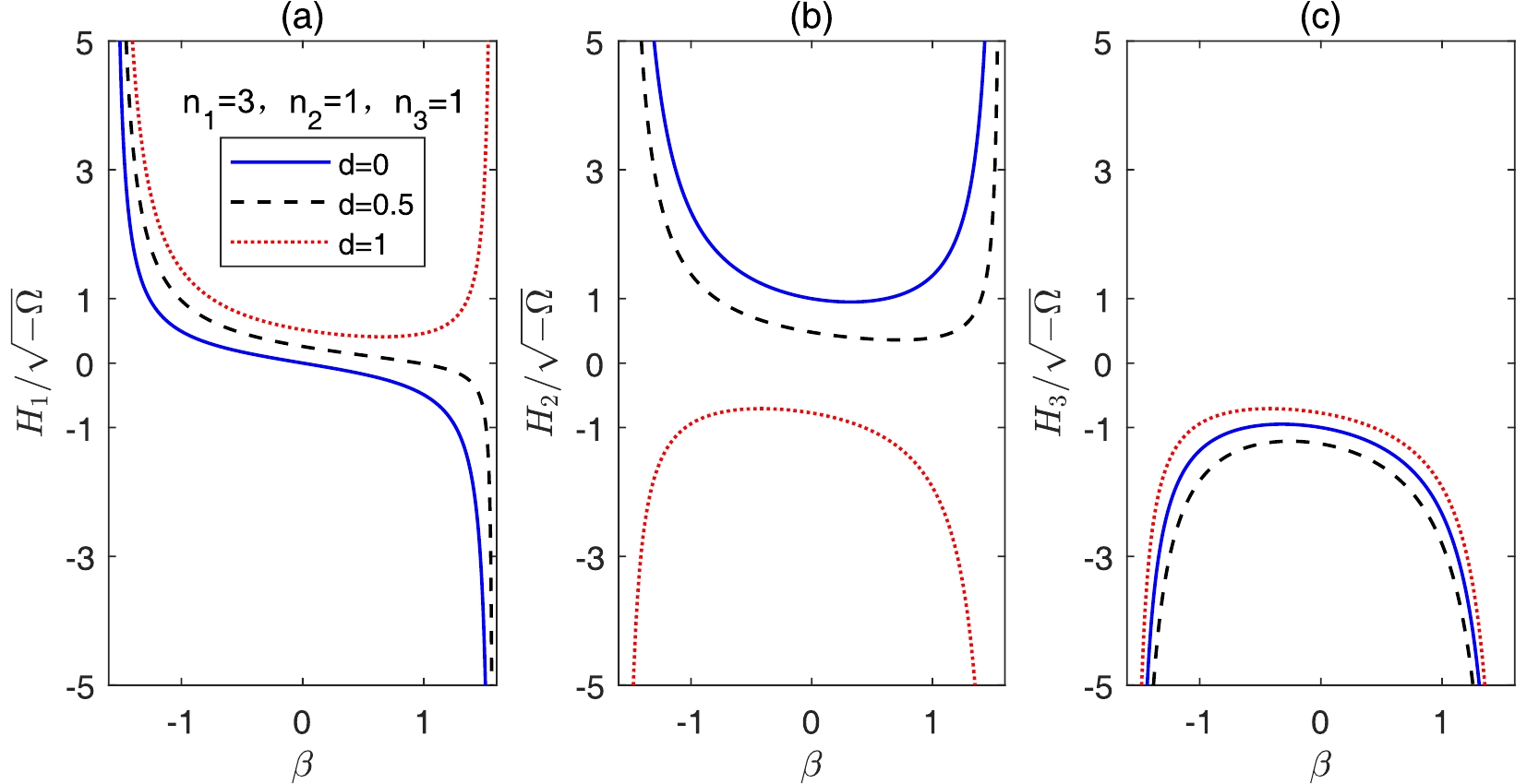
Figure 1. (color online) The Hubble parameters
$ H_{1} $ ($ n_{1} = 3 $ ),$ H_{2} $ ($ n_{2} = 1 $ ), and$ H_{3} $ ($ n_{3} = 1 $ ), with three different parameter values d. (a) The Hubble parameters$ H_{1} $ with$ d = 0, 0.5, 1 $ correspond to the solid (blue) curve, the dashed (black) curve, and the dotted curve (red) respectively ($ n_{2} = 1 $ ). (b)-(c) The case for the Hubble parameters$ H_{2} $ and$ H_{3} $ , respectively.$d > \sqrt{n_{1}/[(n_{2}+n_{3})(n-2)]}\equiv d_{\rm min} = \sqrt{6}/4\approx0.612$

for
$ n_{1} = 3 $ ,$ n_{2} = 1 $ , and$ n_{3} = 1 $ , the Hubble parameter$ H_{1} $ has a minimum$ H_{\rm 1min} = \frac{\sqrt{c^2(n-1)^2-\chi_{1}^{2}}}{n-1}, $

(32) when the term
$ \beta $ in Eq. (22) takes the form$ \beta_{\rm min} = \arcsin \left[\frac{\chi_{1}}{c(n-1)}\right]. $

(33) If
$\beta\leq\beta_{\rm min}$ , the Hubble parameter$ H_{1} $ is a monotonic function decreasing with time, which is not in accordance with cosmological observations and experiments. As can be seen easily from Fig. 1(a), the the Hubble parameter$ H_{1} $ has a minimum when$d = d_{\rm min}\approx0.612$ . This case may be consistent with the present observations because$ H_{1} $ tends to a constant near the minimum, which can lead to accelerated expansion without the contribution of dark energy (or an inflaton field).Combining Eqs. (18), (22), (28) and (29), we obtain
$ H_{1} = H_{2} $ if c satisfies$ c = \sqrt{\frac{-2\Omega n_{3}}{(n-1)(n_{1}+n_{2})}}\equiv c_{eq}. $

(34) It is shown that
$ H_{2} $ tends toward$ H_{1} $ when$ c\rightarrow c_{eq} $ . In the case$ c = c_{eq} $ , the parameter$ d_{eq} $ is defined as:$ d_{eq} = \frac{c_{eq}}{c_{\rm max}} = \sqrt{\frac{n_{1}n_{3}}{(n_{1}+n_{2})(n_{2}+n_{3})}}. $

(35) For
$ n_{1} = 3 $ ,$ n_{2} = 1 $ , and$ n_{3} = 1 $ ,$ d_{eq} = \sqrt{6}/4\approx0.612 $ . Since the extra dimension in our universe is not observed presently, it cannot be too large, and the current scale of extra dimensions is still outside the observable range. When d is equal to$ d_{eq} $ , the extra dimension Hubble parameter$ H_{2} $ is converted to$ H_{1} $ . This case is inconsistent with the presently observed 3D space. The Hubble parameter$ H_{2} $ of the extra dimensions is plotted in Fig. 1(b) for$ d = 0, 0.5, 1 $ . It can be easily seen that the Hubble parameter$ H_{2} $ has a minimum with$ d = 0 $ and 0.5, which can lead to accelerated expansion of the extra dimensions. We are not interested in this situation because it is not in line with observation. However, the Hubble parameter$ H_{2} $ is always negative with$ d = 1 $ , which ensures that the extra dimensions always exceed the observable range. Note here that the ratio of$d_{\rm min}$ to$ d_{eq} $ is$ \frac{d_{\rm min}}{d_{eq}} = \sqrt{\frac{(n_{1}+n_{2})}{n_{3}(n_{1}+n_{2}+n_{3}-1)}}\leqslant 1, $

(36) where
$d_{\rm min}/d_{eq} = 1$ if and only if$ n_{3} = 1 $ . So we only consider the case$ d\gg d_{eq} $ because then we obtain$d\geqslant d_{\rm min}$ when$ d\geqslant d_{eq} $ .In Fig. 2, we have plotted the parameter
$ d_{eq} $ versus the number of extra dimensions$ n_{2} $ and$ n_{3} $ , respectively. The figure on the left is the curve of the parameter$ d_{eq} $ with$ n_{3} $ when$ n_{2} = 1 $ , 5, and 30. It is shown that$ d_{eq} $ monotonically increases with$ n_{3} $ . The parameter$ d_{eq} $ tends toward$ \sqrt{n_{1}/(n_{1}+n_{2})} $ in the$ n_{3}\rightarrow\infty $ limit. In particular,$ d_{eq}\rightarrow\sqrt{3}/2\approx0.866 $ for$ n_{2} = 1 $ . The figure on the right depicts the evolution of$ d_{eq} $ with$ n_{2} $ when$ n_{3} = 1 $ , 5, and 30. In this case,$ d_{eq} $ monotonically decreases with$ n_{2} $ . The parameter$ d_{eq}\rightarrow0 $ in the$ n_{2}\rightarrow\infty $ limit. To be consistent with observation, we should set d to be greater than$ 0.866 $ and closer to 1. Furthermore, we set the constant$ d = 0.98 $ in the following.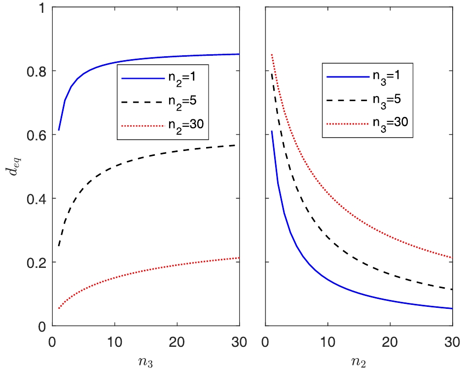
Figure 2. (color online) The parameter
$d_{eq}$ versus the number of extra dimensions$n_{2}$ and$n_{3}$ , respectively. The figure on the left is the curve of the parameter$d_{eq}$ with$n_{3}$ when$n_{2} = 1, 5, 30$ , and the figure on the right depicts the evolution of$d_{eq}$ with$n_{2}$ when$n_{3} = 1, 5, 30$ .In Fig. 3(a)-(c), we plot the Hubble parameters
$ H_{1} $ ,$ H_{2} $ and$ H_{3} $ as a function of$ \beta $ with$ n_{1} = 3 $ when$ d = 0.98 $ . From top to bottom, the three curves having same type (color) corresponds to$ H_{1} $ ,$ H_{2} $ , and$ H_{3} $ , respectively, for fixed values of$ n_{2} $ and$ n_{3} $ . In Fig. 3(a), we plot the Hubble parameter as a function of$ \beta $ at$ n_{2} = 1 $ . From top to bottom, the three solid curves correspond to$ H_{1} $ ,$ H_{2} $ , and$ H_{3} $ at$ n_{3} = 1 $ . The three dashed curves ($ n_{3} = 3 $ ) and the three dotted curves ($ n_{3} = 5 $ ) are similar to the above case. The Hubble parameter of the extra dimensions is always negative at$ n_{3} = 1 $ . With the increase of$ n_{3} $ , the coordinate of the minimum value of$ H_{1} $ tends toward$ \beta = 0 $ . Meanwhile,$ H_{2} $ changes from positive to negative in the region near$ \beta\sim-1.5 $ and$ H_{3} $ is closer to zero. In Fig. 3(b) and (c), the Hubble parameters as a function of$ \beta $ are shown with$ n_{2} = 3 $ and$ n_{2} = 5 $ .$ H_{2} $ is always negative with$ n_{2} = 5 $ , which is similar to the situation in Fig. (1) of Ref. [48].$ H_{1} $ has a lower bound$H_{\rm 1min} = \sqrt{0.98^{2}c_{\rm max}^{2}-\chi_{1}^{2}/(n-1)^{2}}$ when$\beta_{\rm min} = \arcsin\{\eta_{1}/[0.98(n-1)c_{\rm max}]\}$ . In the region near$\beta_{\rm min}$ , we find that$\Omega_{\rm eff} > 0$ is of order$ -\Omega $ . This situation is similar to the case with two different scale factors, and the negative induced cosmological constant$ \Omega $ can be transformed into the positive effective cosmological constant$\Omega_{\rm eff}$ . This tells us that the observed current cosmic acceleration is intrinsically an extra-dimensional phenomenon rather than dark energy. The cosmological constant fine tuning problem can be solved by this extra-dimensional evolution.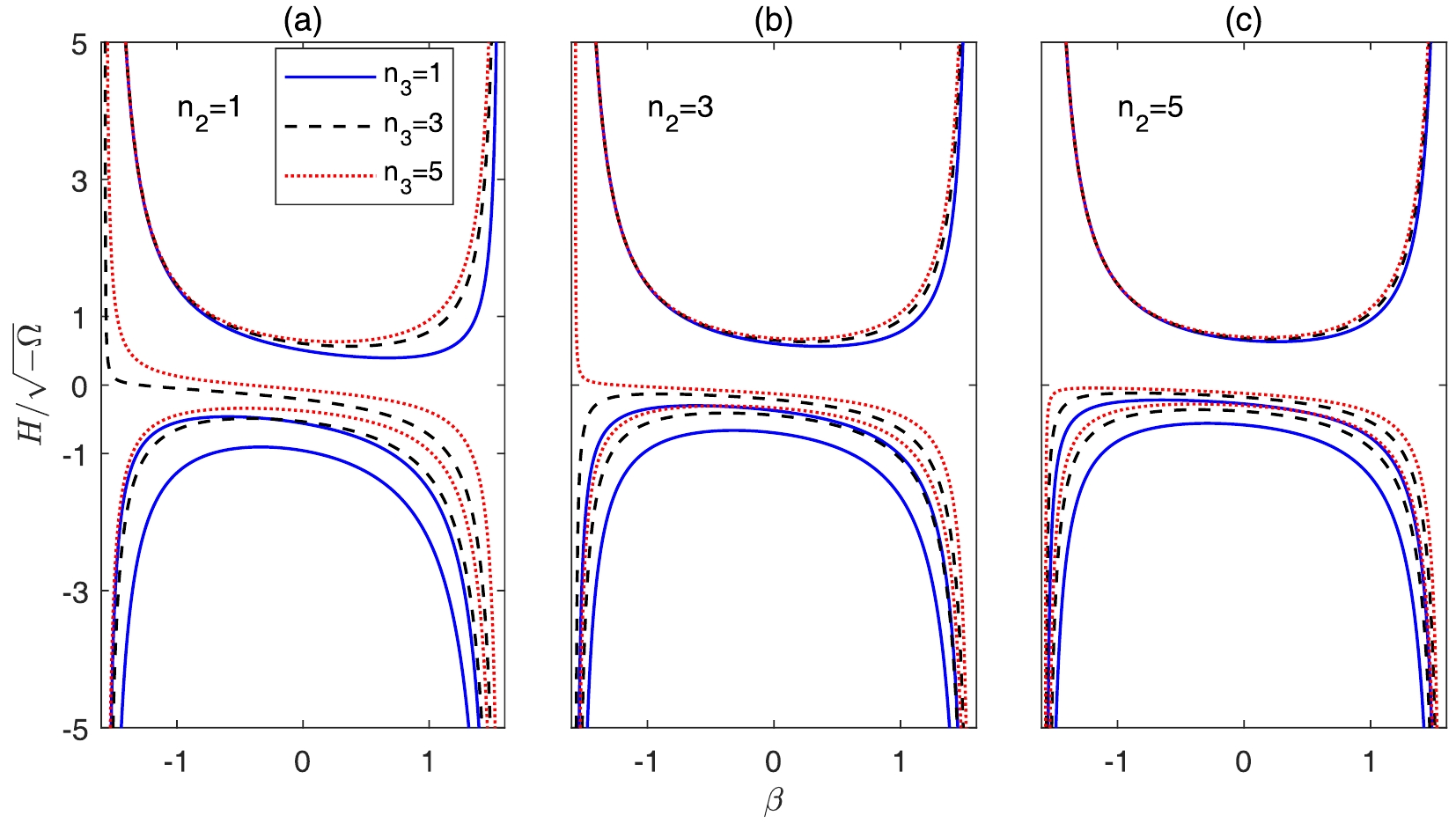
Figure 3. (color online) The Hubble parameters
$ H_{1} $ ($ n_{1} = 3 $ ),$ H_{2} $ , and$ H_{3} $ when$ d = 0.98 $ . (a) The Hubble parameters with$ n_{3} = 1, 3, 5 $ correspond to the solid (blue) curve, the dashed (black) curve and the dotted curve (red) respectively ($ n_{2} = 1 $ ). (b)-(c) The cases for$ n_{2} = 3 $ and$ n_{2} = 5 $ , respectively.From Eqs. (22), (26), and (28) we can get the scale factors
$ a_{1} $ ,$ a_{2} $ , and$ a_{3} $ of the form$ a_{1} = a_{10}|\cos\beta|^{\textstyle\frac{1}{n-1}}|\sec\beta+\tan\beta|^{\textstyle\frac{c}{\chi_{1}}}, $

(37) $ a_{2} = a_{20}|\cos\beta|^{\textstyle\frac{1}{n-1}}|\sec\beta+\tan\beta|^{\textstyle\frac{\chi_{2}-n_{1}c}{\chi_{1}(n_{2}+n_{3})}}, $

(38) $ a_{2} = a_{30}|\cos\beta|^{\textstyle\frac{1}{n-1}}|\sec\beta+\tan\beta|^{\textstyle-\frac{\chi_{3}+n_{1}c}{\chi_{1}(n_{2}+n_{3})}}, $

(39) where
$ a_{10} $ ,$ a_{20} $ , and$ a_{30} $ are the scale factors when the brane forms. Further, since the volume of the visible brane is obtained by$ V_{b} = a_{1}^{n_{1}}a_{2}^{n_{2}}a_{3}^{n_{3}} = a_{10}^{n_{1}}a_{20}^{n_{2}}a_{30}^{n_{3}}\cos\beta, $

(40) when the brane is just forming, there is no particular reason to make the scale factor different, so we choose
$ a_{10} = a_{20} = a_{30} $ . If the initial scale of the brane is of order$ 10^{35} $ in Planck units, and considering the presently observed scale of our universe (of approximate order$ 10^{61} $ ), we obtain the scale of extra dimension which is at least of order$ 10^{22} $ with$ n_{2} = n_{3} = 3 $ . It can be shown that the scale of the extra dimension should be much larger than the Planck length. This ensures that physics is still valid in the evolution of the visible brane. The$ \theta_{0} $ we obtain is close to$ -\pi/2 $ if one wants to have a sufficiently small initial scale. So in the region of$ \theta_{0}+\pi/2\ll\eta_{1}t\ll\pi/2 $ , the Hubble parameter$ H_{1} $ is of the form:$ \begin{split} H_{1}\simeq & \left[\frac{c}{\chi_{1}}+\frac{1}{n-1}\right]\frac{1}{t} \\ =& \frac{1}{n-1}\left[1+d\sqrt{\frac{(n_{2}+n_{3})(n-2)}{n_{1}}}\right]\frac{1}{t}. \end{split} $

(41) When
$ n_{2} = n_{3} = 1 $ and$ d = 0.98 $ ,$ H_{1} $ is about$ 0.52t $ , which is as similar to the radiation dominant era. In the limit$ n_{2}\rightarrow\infty $ (or$ n_{3}\rightarrow\infty $ ),$ H_{1}\simeq\sqrt{3}d/3t $ . -
In conclusion, we investigate an
$ (n+1) $ -d generalized Randall-Sundrum model with an anisotropic metric that has three different scale factors. In this model, we obtain the positive effective cosmological constant$\Omega_{\rm eff}\sim10^{-124}$ (in Planck unit), which only needs a solution$ kr\simeq50-80 $ without fine tuning. This is consistent with the case of two different scale factors.In this model, the Hubble parameter
$ H_{2} $ tends toward$ H_{1} $ when the integration constant d tends toward$ d_{eq} $ . This indicates that the Hubble parameter of observable dimensions is related to the value of the integral constant d. For convenience, here we have selected the Hubble parameter$ H_{1} $ to show the observable dimensions. To be consistent with observation, we should set d to be greater than$ 0.866 $ and closer to 1. Further setting the constant$ d = 0.98 $ , we obtain that$ H_{1} $ has a lower bound$H_{\rm 1min} = \sqrt{0.98^{2}c_{\rm max}^{2}-\chi_{1}^{2}/(n-1)^{2}}$ when$\beta_{\rm min} = \arcsin \{\eta_{1}/[0.98(n-1)c_{\rm max}]\}$ . Meanwhile, the scale of extra dimension is smaller than the observed scale but greater than the Planck length. This may suggest that the observed current cosmic acceleration is caused by extra-dimensional evolution rather than dark energy (or an inflaton field). Of course, there are still many problems to be solved in this model. This includes the question of how the quantum fluctuations contribute to the amount of the expected value of the cosmological constant.
Cosmic acceleration caused by the extra-dimensional evolution in a generalized Randall-Sundrum model
- Received Date: 2020-03-23
- Accepted Date: 2020-07-06
- Available Online: 2020-11-01
Abstract: We investigate an


 DownLoad: