Revisiting nonfactorizable contributions to factorization-forbidden decays of B mesons to charmonium

1. Introduction

• 1. Introduction
• 2. Analytic formulas
• 3. Numerical results
• 4. Conclusion
• Appendix A: Meson distribution amplitudes

In the Standard Model (SM) of particle physics, the charmonium decays of B meson arise from the quark-level process $b\rightarrow q c\bar{c}$ with $q = d,s$, involving tree and penguin amplitudes. The S-wave charmonium states are produced from a $c\bar c$ system with the orbital angular momentum $L = 0$, such as $\eta_c$ and $J/\psi$. These decays belong to the color-suppressed category and receive large nonfactorizable contributions. For the orbital excitation of the $c\bar c$ assignments with $L = 1$, the spin and orbit interaction between the charm-anticharm quarks pair can create four P-wave charmonium states, namely, $\chi_{c0}$, $\chi_{c1}$, $\chi_{c2}$, and $h_c$. Except for the $\chi_{c1}$ modes, which are allowed under the factorization hypothesis, other modes are prohibited because of the $V-A$ structure of the weak vertex [1, 2], where V and A denote the vector and axial vector currents, respectively. However, these processes can occur through a gluon exchange between the charmonium system and the quark in other mesons, which induces the so-called nonfactorizable contributions [2]. Therefore, the factorization-forbidden decays of B meson to a P-wave charmonium state can provide valuable insights into the nonfactorizable mechanism.

Experimentally, the first observation of the decay $B^+ \rightarrow \chi_{c0} K^+$ was reported by the Belle Collaboration [3] using $\chi_{c0}$ decays to the pion or kaon pair, later confirmed by the $BABAR$ Collaboration [4]. Subsequently, both the $BABAR$ [5-8] and Belle Collaborations [9, 10] performed improved measurements. The current world averages of the absolute branching ratio $B \rightarrow \chi_{c0} K$ have reached the order of $10^{-4}$ [11], which is of the same order of magnitude as that of the factorization-allowed $\chi_{c1}$ mode. The corresponding vector $K^*$ mode has been searched for and observed by the $BABAR$ Collaboration [12, 13] with a similar rate. Another factorization-inhibited decay, $B^+\rightarrow \chi_{c2}K^+$, has been measured by the Belle [14, 15] and $BABAR$ [16] Collaborations with an average branching ratio of $(1.1\pm0.4)\times 10^{-5}$ [11], which is an order of magnitude smaller than that of the $\chi_{c0}$ mode. Several collaborations have also searched for the process $B\rightarrow h_c K$ [17-19]. The upper limit of the current branching ratio is $3.8\times 10^{-5}$ at 90% confidence level [11], obtained during the search for $h_c$ by the Belle Collaboration [17]. Very recently, the Belle Collaboration performed a search for the decays $B^+\rightarrow h_c K^+$ and $B^0\rightarrow h_c K^0_S$ [20]. They found evidence for the former with a $4.8\sigma$ significance and set an upper limit on the latter. These results are comparable to $B\rightarrow \chi_{c2} K$ but below the measured rate for $B\rightarrow \chi_{c0} K$. Most recently, both the Belle [21] and $BABAR$ [22] Collaborations present the measurement of the absolute branching fractions of $B^+\rightarrow X_{cc} K^+$, where $X_{cc}$ refers to a charmonium state.

The measured branching ratios in these factorization-inhibited decays are surprisingly larger than the expectations from factorization, which suggests that the nonfactorizable contributions in B decays to charmonium can be sizable. Several attempts have been made to address these challenges. Meli$\acute{c}$ analyzed the effects of soft nonfactorization on $B\rightarrow (\eta_c,J/\psi,\chi_{c0,c1})K$ decays [1] using the light-cone sum rules (LCSR) approach. The calculated branching ratio of the reaction $B\rightarrow \chi_{c0}K$, however, is too small to accommodate the data because of the larger cancellation between the twist-3 and twist-4 pieces in the nonfactorizable contributions. A similar conclusion is also drawn in [23] using the same method. The exclusive B decays to the P-wave charmonium states have been studied within the framework of QCD factorization (QCDF) [24-29]. It was found that the soft contributions may be large, as infrared divergences arise from vertex corrections as well as endpoint singularities owing to the leading twist spectator corrections. However, Beneke pointed out that the concerned decays may occur through the color octet mechanism [30], and the endpoint divergence in hard spectator scattering factorizes and can be absorbed into color octet operator matrix elements [31]. The $B\rightarrow \chi_{c0} K$ and $B\rightarrow h_c K$ decays [32, 33] have been investigated under the perturbative QCD (PQCD) approach based on the $k_T$ factorization theorem [34-37], in which the vertex corrections are ignored and the endpoint singularity is cured by including the parton's transverse momentum. Without endpoint singularity, the PQCD approach has so far been successfully applied to the studies of various factorization-allowed charmonium decays of the B meson [38-50]. Most predictions are consistent with the current experiments. Under another approach [51, 52], by considering intermediate charmed meson rescattering effects, the authors claimed that the rescattering effects could provide the large part of the $B\rightarrow \chi_{c0}K, h_c K$ amplitudes.

Generally, the nonfactorizable dynamics include both the vertex corrections and spectator amplitudes. We agree with the comment made in [32]: the PQCD formalism for the vertex corrections requires the charmonium meson wave functions, dependent on the transverse momenta, as the necessary nonperturbative inputs, which are not yet available completely. The authors of [27] confirm that the vertex corrections are numerically small, and the spectator corrections are large and dominant in the QCDF. Furthermore, the previous PQCD calculations [32, 33] demonstrate that the spectator contributions are sufficient to account for the measurements. Motivated by the same idea, we have reason to believe that it is appropriate to analyze other factorization-inhibited decays, such as $B\rightarrow \chi_{c2} K$, in the PQCD approach. Moreover, we update the P-wave charmonium distribution amplitudes (DAs) based on our previous study [53], where the new universal nonperturbative objects are successful in describing the P-wave charmonium decays of the $B/B_c$ meson [53-55].

The layout of this paper is as follows: In Section 2, we present our theoretical formulae based on the PQCD framework. The input parameters together with the numerical results and discussions are presented in Section 3. Finally, we present the summary in Section 4. The relevant meson distribution amplitudes are presented in the Appendix.

2. Analytic formulas

• 1. Introduction
• 2. Analytic formulas
• 3. Numerical results
• 4. Conclusion
• Appendix A: Meson distribution amplitudes

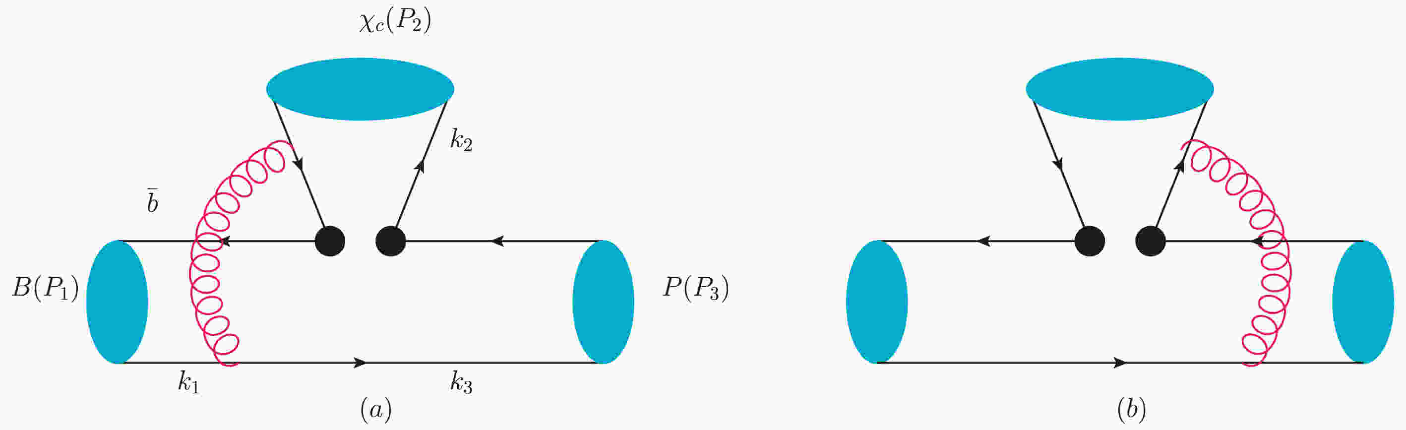
For the factorization-inhibited B decays in question, only the nonfactorization spectator diagrams contribute, which are displayed in Fig. 1. In the rest frame of the B meson, we define $P_i$ and $k_i$ for $i = 1, \;2, \;3$ to be the four-momenta of the mesons and quarks in the initial and final states, as indicated in Fig. 1. In terms of the light-cone coordinates, they are parametrized as [55]

Figure 1

Figure 1.  (color online) Nonfactorizable spectator diagrams for decays $B\to \chi _{c} P$, where P stands for final-state hadron, pion, or kaon.

DownLoad: Full-Size Img PowerPoint

where $r = m/M$ represents the ratio of the charmonium mass m to the B meson mass M. We neglect the light pseudoscalar meson mass for simplicity. $x_i$ and $k_{iT}$ represent the parton longitudinal momentum fractions and parton transverse momenta, respectively. Similar to the vector charmonium, the longitudinal polarization vectors $\epsilon_L$ of an axial-vector charmonium can be defined as

which satisfy the normalization $\epsilon^2_{L} = -1$ and the orthogonality $\epsilon_{L} \cdot P_2 = 0$. For a tensor charmonium, the polarization tensor $\epsilon_{\mu\nu}(\lambda)$ with helicity $\lambda$ can be constructed via the polarization vector $\epsilon_{\mu}$ [56-58], whose detail expressions can be found in Refs. [53, 54].

The Hamiltonian referred to in the SM is written as [59]:

where $G_F$ is the Fermi coupling constant and $\xi_{c(t)} = V^*_{c(t)b}V_{c(t)q}$ is the production of the Cabibbo-Kobayashi-Maskawa (CKM) matrix element. $O_i(\mu)$ and $C_i(\mu)$ are the local four-quark operators and their QCD-corrected Wilson coefficients at the renormalization scale $\mu$, respectively. Their explicit expressions can be found in Ref. [59].

In the PQCD approach, the decay amplitudes are expressed as the convolution of the hard kernel H with the relevant meson light-cone wave functions $\Phi_i$

where “Tr” denotes the trace over all Dirac structures and color indices. t is the energy scale in the hard function H. The meson wave functions $\Phi$ absorb the nonperturbative dynamics in the hadronization processes. For definitions of the P-wave charmonium wave functions, please refer to our previous study [53], whereas for those of B and light pseudoscalar mesons, one can consult Ref. [60]. We list the relevant meson distribution amplitudes and the corresponding parameters in the Appendix. As mentioned before, because only the nonfactorizable spectator diagrams contribute to the hard kernel H, the momentum convolution integral in Eq. (4) would involve all the initial and final states altogether. The perturbative calculations can be performed without endpoint singularity. In the following, we compute the amplitudes of the concerned decays.

We mark subscripts S, A, and T to denote the scalar, axial-vector, and tensor charmonium in the final states, respectively. The decay amplitudes for $(V-A)\otimes(V-A)$ operators read as

with the color factor $C_f = 4/3$ and mass ratios $r_{c} = m_{c}/M$ and $r_p = m_0/M$, where $m_c$ is the charm quark mass and $m_0$ is the chiral scale parameter. For simplicity, in the above formulas, we have combined the two decay amplitudes in Fig. 1(a) and 1(b), because their hard kernels are symmetric under $x_2 \leftrightarrow 1-x_2$, and dropped the power-suppressed terms of order higher than $r^2$. $\alpha$ and $\beta$ represent the virtuality of the internal gluon and quark, respectively, expressed as

The hard scale t is chosen as the largest scale of the virtualities of the internal particles in the hard amplitudes:

The details of the functions h and the Sudakov factors $S_{cd}(t)$ are provided in Appendix A of Ref. [45]. To determine the decay amplitudes from the $(V-A)\otimes(V+A)$ operators, we carry out the Fierz transformation to obtain the appropriate color structure for factorization to work; they satisfy the relations

By combining the contributions from different diagrams with the corresponding Wilson coefficients, we obtain the total decay amplitudes as

and the $CP$-averaged branching ratio is then expressed as

where ${\cal \bar{A}}$ denotes the corresponding charge conjugate decay amplitude, which can be obtained by conjugating the CKM elements in ${\cal A}$.

3. Numerical results

• 1. Introduction
• 2. Analytic formulas
• 3. Numerical results
• 4. Conclusion
• Appendix A: Meson distribution amplitudes

To estimate the contributions from the decay amplitudes, we must specify the various parameters used in our numerical analysis throughout this paper. We employ the meson lifetimes $\tau_{B^+} = 1.638$ ps, $\tau_{B_s} = 1.51$ ps, and $\tau_{B^0} = 1.51$ ps [11]. The parameters relevant for the Wolfenstein parameters are $\lambda = 0.22506$, $A = 0.811$, $\bar{\rho} = 0.124$, and $\bar{\eta} = 0.356$ [11]. We consider $M_B = 5.28$ GeV, $M_{B_s} = 5.37$ GeV, $m_{\chi_{c0}} = 3.415$ GeV, $m_{\chi_{c2}} = 3.556$ GeV, and $m_{h_c} = 3.525$ GeV for the meson masses [11] and $\bar{m}_b(\bar{m}_b) = 4.18$ GeV, $\bar{m}_c(\bar{m}_c) = 1.275$ GeV for the b and c quark “running” masses in the $\overline{MS}$ scheme. The chiral masses relate the pseudoscalar meson mass to the quark mass, which is set as $m_0 = 1.6\pm 0.2$ GeV [61]. The decay constants (GeV) can be extracted from other decay rates or evaluated from the QCD sum rules, which are summarized here [11, 60, 62]:

Using these input parameters and employing the analytic formulas presented in Section 2, we derive the $CP$-averaged branching ratios with error bars as follows:

where the second "equal to" sign in each row denotes the central value with all uncertainties added in quadrature. The theoretical errors correspond to the uncertainties owing to the shape parameters (1) $\omega_b = 0.40\pm 0.04$ GeV for the B meson and $\omega_b = 0.50\pm 0.05$ GeV for the $B_s$ meson, (2) decay constant of the $B/B_s$ meson, which is expressed in Eq. (13), (3) chiral scale parameter $m_0 = 1.6\pm 0.2$ GeV [61] associated with the kaon or pion, which reflects the uncertainty in the current quark masses, (4) heavy quark masses $m_{c(b)}$ within a 20% range, and (5) hard scale t, defined in Eqs. (5)-(7), which we vary from $0.75t$ to $1.25t$, and $\Lambda^{(5)}_{\rm QCD} = 0.25\pm 0.05$ GeV. In general, the uncertainties induced by these parameters are comparable. The uncertainties stemming from the decay constants of charmonium states are not presented explicitly, which affect the branching ratios via the relation ${\cal B}\propto f_{\chi_c}^2$. We have matched the sensitivity of the branching ratios to the charm quark velocity v inside the charmonium DAs in Eq. (A4). The variation of $v^2$ in the range 0.25-0.35 indicates that the difference in our results does not exceed 10%, which suggests that the relativistic corrections may not be significant for these decays.

Further, because isospin is conserved in the heavy quark limit, we can obtain the branching ratios of the neutral counterpart by multiplying the charged ones by the lifetime ratio $\tau_{B^0}/\tau_{B^+}$:

From Eqs. (5)-(7), it can be seen that each decay amplitude receives contributions from both the twist-2 and twist-3 DAs of the charmonium state, the results of which are displayed separately in Table 1, with all the input parameters considered at their central values. We simply symbolize them as “twist-2” and “twist-3”, respectively, while the label “total” corresponds to the total contributions. The numerical results indicate that the dominant contribution comes from the twist-2 DA. This can be understood from the formulas expressed in Eqs. (5)-(7): the contribution of the twist-3 DA is power-suppressed as compared to that of the twist-2 DA. As we have used the same asymptotic model of the twist-2 DA for the three charmonium states [see Eq. (A3)], these decay amplitudes are governed by their different decay constants. The relation among the decay constants $f_{\chi_{c0}}>f_{\chi_{c2}}\sim f_{h_c}$ expressed in Eq. (13) roughly implies the hierarchy pattern presented in Table 1. For the twist-3 piece, the various asymptotic behaviors and tensor decay constants contribute to different values.

Table 1

Table 1.  Values of decay amplitudes from twist-2 and twist-3 charmonium distribution amplitudes for $B^+\rightarrow (\chi_{c0},\chi_{c2},h_c)K^+$ decays. Results are given in units of $10^{-3}$ GeV³.

Decay amplitudes	Twist-2	Twist-3	Total
${{\cal A}(B^+ \rightarrow \chi_{c0} K^+) }$	13 + 21i	− 4 − 4i	9 + 17i
${ {\cal A}(B^+ \rightarrow \chi_{c2} K^+) }$	5.9 + 8.3i	− 0.2 − 0.6i	5.7 + 7.7i
${ {\cal A}(B^+ \rightarrow h_c K^+) }$	5.9 + 8.5i	− 1.1 + 0.2i	4.8 + 8.7i

DownLoad: CSV

Show Table

As discussed in Refs. [63, 64], for the nonleptonic two-body decay of the B meson, if the emitted particle from the weak vertex is a pseudoscalar or vector meson, there is a destructive interference between the two nonfactorizable spectator diagrams presented in Fig. 1 owing to the symmetric twist-2 DAs of the emitted meson. However, in this study, all the twist-2 DAs of the emitted charmonium state are antisymmetric under the exchange of the momentum fractions $x_2$ of the c quark and $1-x_2$ of the $\bar c$ quark [see Eq. (A3)], which reverses the constructive or destructive interference situation. To be more explicit, we present the values of two spectator amplitudes in Table 2, where ${\cal A}_a$ and ${\cal A}_b$ denote the decay amplitudes from Fig. 1(a) and Fig. 1(b), respectively. It can be seen that the constructive interference between ${\cal A}_a$ and ${\cal A}_b$ can enhance the total decay amplitudes. Therefore, the large decay rates for these factorization-forbidden modes are comparable to those naively factorizable decays.

Table 2

Table 2.  Values of decay amplitudes from nonfactorizable diagrams (a) and (b) for $B^+\rightarrow (\chi_{c0},\chi_{c2},h_c)K^+$ decays. Results are presented in units of $10^{-3}$ GeV³.

Decay amplitudes	${ {\cal A}_a }$	${ {\cal A}_b }$	Total
${ {\cal A}(B^+ \rightarrow \chi_{c0} K^+) }$	3 + 3i	6 + 14i	9 + 17i
${ {\cal A}(B^+ \rightarrow \chi_{c2} K^+) }$	3.3 + 0.4i	2.4 + 7.3i	5.7 + 7.7i
${ {\cal A}(B^+ \rightarrow h_c K^+) }$	1.8 + 0.5i	3.0 + 8.2i	4.8 + 8.7i

DownLoad: CSV

Show Table

To make a comparison, we also collect the various available theoretical predictions evaluated in LCSR [1, 23], QCDF [26-28, 31], and PQCD [32, 33] as well as the current world average values from the PDG [11] presented in Table 3. The LCSR calculations mainly focus on the ${\cal B}(B^+ \rightarrow \chi_{c0} K^+)$ decay. There are lager discrepancies in their numerical results [1, 23]. The LCSR prediction of ${\cal B}(B^+ \rightarrow \chi_{c0} K^+)\sim 10^{-7}$ [1] is far too small and clearly ruled out by experiment. Three QCDF calculations exist for the concerned decays. As mentioned in the Introduction, the QCDF suffers the infrared divergences arising from the vertex diagrams and endpoint divergences owing to spectator amplitudes in the leading-twist order. The main reason for the different numerical results is the treatment of these divergences. In [27], the infrared and endpoint divergences were regularized by a nonzero gluon mass and the off-shellness of the quarks, respectively. The authors found that the $B\rightarrow \chi_{c0} K$ is dominated by the spectator contribution, whereas the contributions arising from the vertex are numerically small. Subsequently, the same scheme is applied to the $B\rightarrow h_c(\chi_{c2}) K$ decays [28] with the exception of neglecting the vertex corrections. In Ref. [31], the authors used the space-time dimension as the infrared regulator, whereas the endpoint divergence was absorbed into the color octet operator matrix elements. The scheme used in [26] is that a nonzero binding energy is introduced to regularize the infrared divergence, and the spectator contributions are parameterized in a model-dependent way. In general, our results are more consistent with the QCDF predictions from [31] within the low charm quark mass region. Compared with previous PQCD calculations [32, 33], we update the charmonium distribution amplitudes and some input parameters in this study. Our predictions on ${\cal B} (B\rightarrow \chi_0 K)$ yield typically smaller values than those of [32] and are closer to the current experimental average [11]. For the $h_c$ mode, both the current PQCD result and the previous calculations from [28, 33] are well consistent with the present data. Two earlier papers [51， 52] studied the decays of $B^+ \rightarrow \chi_{c0} K^+$ and $B^+ \rightarrow h_c K^+$ by including the rescattering effects. The evaluated branching ratios lie in the ranges $(1.1\sim 3.5)\times$$10^{-4}$ and $(2\sim 12)\times 10^{-4}$, respectively. Although the rescattering effects can enhance the branching ratio of $B^+ \rightarrow \chi_{c0} K^+$ to match the data, the value of ${\cal B}(B^+ \rightarrow h_c K^+)$ may be overestimated owing to uncontrollable theoretical uncertainties.

Table 3

Table 3.  Branching ratios (in units of ${ 10^{-4} }$) of Cabibbo-favored decays from various theoretical studies in literature [1, 23, 26-28, 31-33]. Data have been taken from PDG 2018 [11].

Modes	This study	LCSR	QCDF	PQCD	Data [11]
${ B^+ \rightarrow \chi_{c0} K^+ }$	${ 1.4^{+1.3}_{-0.9} }$	${ (1.7\pm 0.2)\times 10^{-3} }$ [1]	${ 0.78^{+0.46}_{-0.35} }$ [26]	5.61 [32]	${ 1.50^{+0.15}_{-0.13} }$
		${ 1.0 \pm 0.6 }$ [23]	${ 2 \sim 4 }$ [27]
			1.05 [28] b
${ B^0 \rightarrow \chi_{c0} K^0 }$	${ 1.3^{+1.2}_{-0.8} }$	–	${ 1.13 \sim 5.19 }$ [31] a	5.24 [32]	${ 1.11^{+0.24}_{-0.21}\times 10^{-2} }$
${ B^+ \rightarrow \chi_{c2} K^+ }$	${ 0.32^{+0.14}_{-0.13} }$	–	${ 1.68^{+0.78}_{-0.69} }$ [26]	–	${ 0.11\pm 0.04 }$
			0.03 [28] b
${ B^0 \rightarrow \chi_{c2} K^0 }$	${ 0.29^{+0.13}_{-0.12} }$	–	${ 0.28 \sim 3.98 }$ [31] a	–	${<0.15 }$
${ B^+ \rightarrow h_c K^+ }$	${ 0.35^{+0.19}_{-0.13} }$	–	0.27 [28] b	0.36 [33]	${ 0.37\pm 0.12 }$
${ B^0 \rightarrow h_c K^0 }$	${ 0.32^{+0.18}_{-0.12} }$	–	${ 0.29 \sim 0.53 }$ [31] a	–	${<0.14 }$ c
aQuoted range represents variation in charm quark mass.bWe quote result with ${\mu=4.4}$ GeV. cCited upper limit ${1.4\times 10^{-5}}$ is for ${B^0\rightarrow h_c K^0_S}$ [20].

DownLoad: CSV

Show Table

From Table 3, one can see that the $B^+ \rightarrow \chi_{c2} K^+$ channel is predicted to have a threefold larger branching ratio when compared with the data, which is dominated by the Belle experiment [15]. $BABAR$ gave the upper bounds (the values) [16] as follows:

where the uncertainties are statistical and systematic, respectively. It seems that their central values are somewhat different and suffer from sizeable statistical uncertainties. Our branching ratio for the neutral mode is comparable with the upper limit of $BABAR$ [16]. It is worth noting that the predictions from QCDF on this mode have a relatively big spread. For example, the QCDF prediction from [28] led to ${\cal B}(B^+ \rightarrow \chi_{c2} K^+) = 3.0\times 10^{-6}$, which is too small compared to the measured value. However, another QCDF prediction, of the order of $10^{-4}$ [26], is too large. As pointed out in [26], the number can be adjusted to the right magnitude with an appropriate choice for the parameters of the spectator hard scattering contributions. The large numerical difference between the two QCDF calculations is mainly caused by the large twist-3 spectator contribution, which can be traced to the infrared behavior of the spectator interactions.

As mentioned above, the charged and neutral decay modes differ in the lifetimes of $B^0$ and $B^+$ in our formalism; the predicted branching ratios have almost the same magnitude. However, the data of ${\cal B}(B^0 \rightarrow \chi_{c0} K^0)$ in Table 3 is two orders of magnitude smaller than those of the charged one. This number was obtained in the LHCb experiment from the Dalitz plot (DP) analysis of the $B^0\rightarrow K_S^0\pi^+\pi^-$ decays [65]. It indicates a tension with the similar amplitude analysis performed in the $BABAR$ experiment [8, 66, 67]. One can see that all the model calculations in Table 3 are substantially larger in magnitude than the LHCb data. Improved measurements are certainly needed for this decay mode.

The decays with $\pi$ and $\bar K$ in the final state have relatively small branching ratios ($\sim 10^{-6}$) owing to the CKM factor suppression. Experimentally, only the $BABAR$ collaboration reported the upper limits of the branching ratio products ${\cal B}(B^+\rightarrow \chi_{c0,c2})\times {\cal B}(\chi_{c0,c2}\rightarrow \pi^+\pi^-) <1.0 \times 10^{-7}$ by applying DP analysis on the charmless decay $B\rightarrow$$\pi\pi\pi$. Combining the experimental facts ${\cal B}(\chi_{c0}\rightarrow \pi^+\pi^-) =$$\dfrac{2}{3}(8.51\pm 0.33)\times 10^{-3}$ and ${\cal B}(\chi_{c2}\rightarrow \pi^+\pi^-) = \dfrac{2}{3}(2.23\pm 0.09)\times$$10^{-3}$ [11], where the factors of $2/3$ are attributed to isospin, we can infer the experimental upper bounds:

There is substantial room for our predictions to reach the experimental upper limits. As these Cabibbo-suppressed decays have received less attention in other approaches, we await future comparisons.

The $CP$ asymmetry arises from the interference between the tree and penguin amplitudes. Using the same definition as that in Ref. [55], we study direct $CP$ violation $A^{\rm{dir}}_{CP}$ and mixing-induced $CP$ asymmetry S for the decays in question. The two $CP$-violating parameters can be expressed as

with $\lambda_f = \eta_f {\rm e}^{-2{\rm i}\beta_{(s)}}\dfrac{{\cal \bar{A}}}{{\cal A}}$ and $\eta_f = 1(-1)$ for $CP$-even (odd) final states. $\beta_{(s)}$ is one of the angles of the unitarity triangle in the CKM quark-mixing matrix [11]. Our numerical results are tabulated in Table 4, where the errors are induced by the same sources as the ones expressed in Eq. (14). As the hadronic parameter dependence cancels out in Eq. (18), these $CP$ asymmetries are more sensitive to the heavy quark masses and the hard scale. It is evident that direct $CP$ violations for decays involving K are very small, of the order of $10^{-4}$, owing to an almost null weak phase from the CKM matrix element $V_{ts}$. For other channels, the weak phase from $V_{td}$ will enhance $A^{\rm{dir}}_{CP}$ substantially to the level of $10^{-2}$. Because the penguin contribution is small compared to that of the tree, the mixing-induced $CP$ asymmetry S in Eq. (18) is approximately expressed as $-\eta_f S\approx \sin(2\beta)$. It is clear from Table 4 that the predicted values of S are not significantly different from the current world average values $\sin(2\beta) = 0.695\pm0.019$ and $2\beta_s = (2.55\pm 1.15)\times 10^{-2}$ [11]. With further experimental data in the future, these modes can serve as alternatives to extract the CKM phases $\beta_{(s)}$.

Table 4

Table 4.  PQCD predictions for ${ CP }$ asymmetry parameters.

Modes	${ A^{\rm{dir}}_{CP} }$	${ S_{f} }$(%)
${ B^0 \rightarrow \chi_{c0} K_S^0 }$	${ -5.5^{+0.1+0.0+0.4+3.3+2.5}_{-0.2-0.0-0.9-2.1-3.2}\times 10^{-4} }$	${ -69.8^{+0.0+0.0+0.0+0.0+0.1}_{-0.0-0.0-0.0-0.0-0.1} }$
${ B^0 \rightarrow \chi_{c2} K_S^0 }$	${ -5.2^{+0.1+0.0+0.2+1.5+2.7}_{-0.0-0.0-0.1-0.0-3.0}\times 10^{-4} }$	${ -69.8^{+0.0+0.0+0.0+0.0+0.1}_{-0.0-0.0-0.0-0.0-0.1} }$
${ B^0 \rightarrow h_c K_S^0 }$	${ 1.3^{+0.0+0.0+0.0+0.2+1.0}_{-0.0-0.0-0.0-0.1-0.7}\times 10^{-4} }$	${ 69.4^{+0.0+0.0+0.0+0.0+0.0}_{-0.0-0.0-0.0-0.0-0.0} }$
${ B^0 \rightarrow \chi_{c0} \pi^0 }$	${ 1.2^{+0.1+0.0+0.3+0.5+0.6}_{-0.0-0.0-0.2-0.7-0.4}\times 10^{-2} }$	${ -63.8^{+0.1+0.0+0.1+0.3+1.0}_{-0.2-0.0-0.2-0.4-0.2} }$
${ B^0 \rightarrow \chi_{c2} \pi^0 }$	${ 9.9^{+0.3+0.0+0.5+0.1+6.1}_{-0.1-0.0-0.5-2.1-5.1}\times 10^{-3} }$	${ -63.6^{+0.1+0.0+0.0+0.5+0.6}_{-0.1-0.0-0.0-0.4-0.6} }$
${ B^0 \rightarrow h_c \pi^0 }$	${ -2.5^{+0.1+0.0+0.1+0.6+1.6}_{-0.0-0.0-0.0-0.0-2.0}\times 10^{-3} }$	${ 70.8^{+0.1+0.0+0.0+0.1+0.2}_{-0.1-0.0-0.0-0.2-0.2} }$
${ B_s^0 \rightarrow \chi_{c0} K_S^0 }$	${ 1.1^{+0.1+0.0+0.3+0.7+0.6}_{-0.1-0.0-0.1-0.7-0.3}\times 10^{-2} }$	${ 4.5^{+0.2+0.0+0.2+0.4+0.7}_{-0.2-0.0-0.2-0.2-0.8} }$
${ B_s^0 \rightarrow \chi_{c2} K_S^0 }$	${ 9.6^{+0.3+0.0+0.2+0.7+3.9}_{-0.7-0.0-0.6-2.8-4.4}\times 10^{-3} }$	${ 4.9^{+0.2+0.0+0.0+0.4+0.8}_{-0.2-0.0-0.0-0.5-0.6} }$
${ B_s^0 \rightarrow h_c K_S^0 }$	${ -2.5^{+0.0+0.0+0.1+0.8+1.3}_{-0.0-0.0-0.1-0.3-1.7}\times 10^{-3} }$	${ 4.2^{+0.0+0.0+0.0+0.1+0.3}_{-0.1-0.0-0.0-0.2-0.3} }$

DownLoad: CSV

Show Table

Experimentally, the world average of $A_{CP}(B^+\rightarrow \chi_{c0}K^+) = -0.20\pm 0.18$ based on the measurements $-0.14\pm 0.15^{+0.03}_{-0.06}$ [6] and $-0.96\pm0.37\pm 0.04$ [7] from $BABAR$ and $-0.065\pm0.20^{+0.035}_{-0.024}$ [10] from Belle. It should be noted that the number from [7] has a large and non-Gaussian uncertainty and its difference from zero is not statistically significant. All measured direct $CP$ violations are consistent with zero. Because LHCb has measured $A_{CP}$ to the accuracy of $10^{-3}$, it is conceivable that an observation of $CP$ violation in other decays will be feasible in the near future. The mixing-induced $CP$ asymmetry for $B^0\rightarrow\chi_{c0}K^0_S$ decay is measured by $BABAR$ [66] with two solutions:

where the last uncertainty represents the dependence of the DP signal model. We can note that the first experimental solution is more favored by our calculation.

4. Conclusion

• 1. Introduction
• 2. Analytic formulas
• 3. Numerical results
• 4. Conclusion
• Appendix A: Meson distribution amplitudes

The factorization-forbidden decays of the B meson to charmonium have been revisited in the PQCD formalism, which is free from endpoint singularities. The charmonium distribution amplitudes are updated based on our previous study. We find that the dominant contribution comes from the leading-twist charmonium distribution amplitudes. The constructive interference between the two nonfactorizable spectator diagrams enhances the decay rate, which can be compatible with the factorization-allowed decays. The obtained branching ratios of the $B^+\rightarrow \chi_{c0} K^+$ and $B^+\rightarrow h_c K^+$ decays are essentially in agreement with the current data, whereas estimates of the $\chi_{c2}$ decays are found to be larger, typically by a factor of 3. For the decays involving $\pi$ or $\bar K$ in the final state not yet measured, the calculated branching ratios will be further tested by the LHCb and Belle-II experiments in the near future. We further estimate the $CP$-violating parameters. As expected, the direct $CP$ asymmetries in these channels are very low owing to the suppressed penguin contributions. The mixing-induced $CP$ asymmetries are close to $\sin(\beta_{(s)})$, which suggests that these channels can provide a cross-check on the measurement of the CKM phases $\beta$ and $\beta_s$.

We have also collected other theoretical results, whenever available, in Table 3 and made a detailed comparison. The predicted branching ratios for most decay processes have similar magnitudes, whereas they can differ by several factors for specific decay modes. In general, our predictions are more consistent with the data compared to these earlier analyses.

We discussed the theoretical uncertainties arising from the hadronic parameters, such as $\omega$, $f_B$, and $m_0$, in the meson wave function, heavy quark masses, and hard scale, which can significantly affect the branching ratios, whereas the $CP$ asymmetries are found to be relatively stable with respect to variations in the hadronic parameters. The reasonably accurate results obtained will be tested at existing and forthcoming hadron colliders.

Appendix A: Meson distribution amplitudes

• 1. Introduction
• 2. Analytic formulas
• 3. Numerical results
• 4. Conclusion
• Appendix A: Meson distribution amplitudes

The light-cone meson distribution amplitudes are, in principle, not calculable in PQCD, but they are universal for all the decay channels. In this Appendix, we present explicit expressions for the meson distribution amplitudes appearing in the decay amplitudes in Section 2. First, for the B meson distribution amplitudes, we adopt the model [36, 37, 60]

with the shape parameters $\omega_b = 0.4$ GeV and $\omega_b = 0.5$ GeV for the B and $B_s$ mesons, respectively. The coefficient N is related to the decay constant $f_B$ by normalization:

The distribution amplitudes of the P-wave charmonium states, defined via the nonlocal matrix element, have been derived in Ref. [53]; we collect their expressions as follows:

where

and v is the charm quark velocity, which denotes the relativistic corrections to the Coulomb wave functions [68]. We consider $v^2 = 0.3$ for charmonium. The normalization constants $N_{L, T, S}$ can be determined using the corresponding normalization conditions [53].

The kaon and pion meson distribution amplitudes up to twist-3 are determined using the light-cone QCD sum rules [61, 69]:

with the Gegenbauer polynomials

The Gegenbauer moments for the twist-2 LCDAs are used with the following updated values at the scale $\mu = 1$ GeV [70]:

References