Constraints on anomalous quartic gauge couplings via Wγjj production at the LHC

Over the past few decades, most of the experimental measurements have been in good agreement with the predictions of the Standard Model (SM). The search for new physics beyond the SM (BSM) is one of the main objectives of current and future colliders. Among the processes measured at the Large Hadron Collider (LHC), vector boson scattering (VBS) processes provide ideal conditions to study BSM. It is well known that the perturbative unitarity of the longitudinal $W_LZ_L\to W_LZ_L$ scattering is violated without the Higgs boson, which sets an upper bound on the mass of the Higgs boson [1]. In other words, with the discovery of the Higgs boson, the Feynman diagrams of the VBS processes cancel each other and the cross sections do not grow with centre-of-mass (c.m.) energy. However, such suppression of the cross section can be relaxed in the presence of new physics particles. Consequently, the cross section may be significantly increased and a window to detect BSM is open [2, 3].

A model-independent approach, called the SM effective field theory (SMEFT) [4-6], has been used widely to search for BSM. In the SMEFT, the SM is a low energy effective theory of some unknown BSM theory. When the c.m. energy is not sufficient to produce the new resonance states directly and when the new physics sector is decoupled, one can integrate out the new physics particles. Then, the BSM effects become new interactions of known particles. Formally, the new interactions appear as higher dimensional operators. The VBS processes are suitable for investigating the existence of new interactions involving electroweak symmetry breaking (EWSB), which is contemplated in many BSM scenarios. The operators w.r.t. EWSB up to dimension-8 can contribute to the anomalous trilinear gauge couplings (aTGCs) and anomalous quartic gauge couplings (aQGCs). There are many full models that contain these operators, for example, anomalous gauge-Higgs couplings, composite Higgs, warped extra dimensions, 2HDM, $U(1)_{L_{\mu}-L_{\tau}}$, as well as axion-like particle scenarios [7-18].

Both aTGCs and aQGCs could impact VBS processes [19-22]. Unlike aTGCs, which also affect the diboson productions and the vector boson fusion (VBF) processes[2, 3, 23, 24], the most sensitive processes for aQGCs are the VBS processes. The dimension-8 operators can contribute to aTGCs and aQGCs independently. Therefore, we focus on the dimension-8 anomalous quartic gauge-boson operators. Moreover, it is possible that higher dimensional operators contributing to aQGCs exist without dimension-6 operators. This situation arises in the Born-Infeld (BI) theory proposed in 1934 [25], which is a nonlinear extension of the Maxwell theory motivated by a "unitarian" standpoint. It could provide an upper limit on the strength of the electromagnetic field. In 1985, the BI theory was reborn in models inspired by M-theory [26, 27]. We note that the constraint on the BI extension of the SM has recently been presented via dimension-8 operators in the SMEFT [28].

Historically, VBS has been proposed as a means to test the structure of EWSB since the early stage of planning for the Superconducting Super Collider (SSC) [29]. The study of VBS has attracted significant attention during the past few years. The first report of constraints on dimension-8 aQGCs at the LHC is from the same-sign $WW$ production [30, 31]. At present, a number of experimental results in VBS have been obtained, including the electroweak-induced production of $Z\gamma jj$, $W\gamma jj$ at $\sqrt{s} = 8\ {{\rm{TeV}}}$ and $ZZjj$, $WZjj$, $W^+W^+jj$ at $\sqrt{s} = 13\ {{\rm{TeV}}}$ [32-39]. Furthermore, theoretical studies have been extensively performed [40-44]. Among these VBS processes, in this paper we consider $W\gamma jj$ production via scattering between $Z/\gamma$ and $W$ bosons. The next-to-leading order (NLO) QCD corrections to the process $pp\to W\gamma jj$ have been computed in Refs. [21, 45], and the K factor has been found to be close to 1 ($K\approx 0.97$ [21]). However, the phenomenology of this process with aQGCs needs further investigation.

The SMEFT is valid only under a certain energy scale $\Lambda$. The validity of the SMEFT with dimension-8 operators is an important issue that has been ignored in previous experiments. The amplitude of VBS with aQGCs increases as ${\cal{O}}(E^4)$, leading to tree-level unitarity violation at high enough energies [46-48]. In such a case, it is inappropriate to use the SMEFT. A unitarity bound should be set to prevent the violation of unitarity. The unitarity bound is often regarded as a constraint on the coefficient of a high dimensional operator. However, this constraint is not feasible in VBS processes because the energy scale of the sub-process is not a fixed value but a distribution. To consider validity, it is proposed that [49] the constraints obtained by experiments should be reported as functions of energy scales. However, in the $W\gamma jj$ production, the energy scale of sub-process $\hat{s} = (p_W+p_{\gamma})^2$ is not an observable. In this study, we obtain an approximation of $\hat{s}$, based on which the unitarity bounds are applied as limits on the events at fixed coefficients. The unitarity bounds will suppress the number of signal events.

To enhance the discovery potentiality of the signal, we have to optimize the event selection strategy. With the approximation of $\hat{s}$, other limits to cut off the small $\hat{s}$ events become redundant. Therefore, we investigate another important feature of the aQGC contributions, namely, the polarization of the $W$ boson and the resulting angular distribution of the leptons. The polarization of the $W$ and $Z$ bosons plays an important role in testing the SM [50]. Angular distribution is a good observable to search for BSM signals (an excellent example is the $P_5'$ form factor [51, 52]) because the differential cross section exposes more information than the total cross section. Although the polarization fractions of the $W$ and $Z$ bosons have been studied extensively within the SM [53-58], the angular distribution caused by the polarization effects of aQGCs needs further investigation.

The paper is organized as follows: in section 2, we introduce the effective Lagrangian and the corresponding dimension-8 anomalous quartic gauge-boson operators relevant to $W\gamma jj$ production in VBS processes, and the experimental constraints on these operators are presented. In section 3, we analyze the partial-wave unitarity bounds. In section 4, we first propose a cut based on the unitarity bound to ensure that the selected events are described correctly using the SMEFT. Next, we discuss the kinematic and polarization features of the signal events as well as the event selection strategy. Based on our event selection strategy, we obtain the constraints on the coefficients of dimension-8 operators with current luminosity at the LHC. In section 5, we present the cross sections and the significance of the aQGC signals in the $\ell\nu\gamma jj$ final state. Finally, we summarize our results in section 6.

The Lagrangian of the SMEFT can be written in terms of an expansion in powers of the inverse of new physics scale $\Lambda$ [4-6]:

where ${\cal{O}}_{6i}$ and ${\cal{O}}_{8j}$ are dimension-6 and dimension-8 operators, respectively, and $C_{6i}/\Lambda ^2$ and $C_{8j}/\Lambda ^4$ are the corresponding Wilson coefficients. The effects of BSM are described by higher dimensional operators, which are suppressed by $\Lambda$. For one generation fermions, 86 independent operators, out of 895 baryon number conserving dimension-8 operators, can contribute to QGCs and TGCs [22].

We list dimension-8 operators affecting the aQGCs relevant to the $W\gamma jj$ production [59, 60]:

with

where $\widehat{W}\equiv \vec{\sigma}\cdot \vec{W}/2$ , $\sigma$ is the Pauli matrix, and $\vec{W}\equiv \{W^1, W^2, W^3\}$.

The tightest constraints on the coefficients of the corresponding operators are obtained via $WWjj$, $WZjj$, $ZZjj$, and $Z\gamma jj$ channels through CMS experiments at $\sqrt{s} = 13$ TeV [61, 62], which are listed in Table 1.

coefficient	constraint		coefficient	constraint
$f_{M_0}/\Lambda ^4\;({{\rm{TeV}}^{-4}})$	$[-0.69,0.70]$ [61]		$f_{T_0}/\Lambda ^4\;({{\rm{TeV}}^{-4}})$	$[-0.12,0.11]$ [61]
$f_{M_1}/\Lambda ^4\;({{\rm{TeV}}^{-4}})$	$[-2.0,2.1]$ [61]		$f_{T_1}/\Lambda ^4\;({{\rm{TeV}}^{-4}})$	$[-0.12,0.13]$ [61]
$f_{M_2}/\Lambda ^4\;({{\rm{TeV}}^{-4}})$	$[-8.2,8.0]$ [62]		$f_{T_2}/\Lambda ^4\;({{\rm{TeV}}^{-4}})$	$[-0.28,0.28]$ [61]
$f_{M_3}/\Lambda ^4\;({{\rm{TeV}}^{-4}})$	$[-21,21]$ [62]		$f_{T_5}/\Lambda ^4\;({{\rm{TeV}}^{-4}})$	$[-0.7,0.74]$ [62]
$f_{M_4}/\Lambda ^4\;({{\rm{TeV}}^{-4}})$	$[-15,16]$ [62]		$f_{T_6}/\Lambda ^4\;({{\rm{TeV}}^{-4}})$	$[-1.6,1.7]$ [62]
$f_{M_5}/\Lambda ^4\;({{\rm{TeV}}^{-4}})$	$[-25,24]$ [62]		$f_{T_7}/\Lambda ^4\;({{\rm{TeV}}^{-4}})$	$[-2.6,2.8]$ [62]
$f_{M_7}/\Lambda ^4\;({{\rm{TeV}}^{-4}})$	$[-3.4,3.4]$ [61]

Table 1.  Constraints on coefficients obtained through CMS experiments.

The aQGC vertices relevant to the$W\gamma jj$ channel are $W^+W^-\gamma\gamma$ and $W^+W^-Z\gamma$, which are

and the coefficients are

Note that vertices $V_{WWZ\gamma,0,1,2,3,4}$ and $V_{AAWW,0,1}$ are dimension-6 derived from $O_{M_i}$, and the other vertices are dimension-8 derived from $O_{T_i}$.

Unlike in the SM, the cross section of the VBS process with aQGCs increases with c.m. energy. Such a feature opens a window to detect aQGCs at higher energies. However, the cross section with aQGCs will violate unitarity at a certain energy scale. The unitarity violation indicates that the SMEFT is no longer appropriate for describing the phenomenon at such high energies perturbatively.

Considering the process $V_{1,\lambda _1}V_{2,\lambda _2}\to V_{3,\lambda _3}V_{4,\lambda _4}$, where $V_i$ are vector bosons, $\lambda _i$ correspond to the helicities of $V_i$, and therefore $\lambda _i = \pm 1$ for photons, and $\lambda _i = \pm 1, 0$ for $W^{\pm},Z$ bosons, its amplitudes can be expanded as [63, 64]

where $V_1$ is $\gamma$ or $Z$ boson, $\lambda = \lambda _1-\lambda _2$, $\lambda ' = \lambda _3-\lambda _4$, $\theta$ and $\phi$ are the zenith and azimuth angles of the $\gamma$ in the final state, $d^J_{\lambda \lambda '}(\theta)$ are the Wigner $d$-functions [63], and $T^J$ are coefficients of the expansion that can be obtained via Eq. (9). Partial-wave unitarity for the elastic channels requires $|T^J|\leqslant 2$ [64], which has been used widely in previous studies [65-68].

We calculate the partial-wave expansions of the $W\gamma\to W\gamma$ amplitudes with one dimension-8 operator at a time. Denoting ${\cal{M}}^{f_{X}}$ as the amplitude with only the$O_X$ operator, for $O_{M_{2,3,4,5,7}}$ and $O_{T_{5,6,7}}$, which can be derived using Eq. (8) as

Therefore, only the partial-wave expansions of amplitudes for the $O_{M_{0,1}}$ and $O_{T_{0,1,2}}$ operators are required to be calculated. The amplitudes increase with the c.m. energy $\sqrt{\hat{s}}$. Retaining only the leading terms, the results are listed in Table 2. There are also leading terms that can be obtained using the relation ${\cal{M}}_{\lambda _1, \lambda _2, \lambda _3, \lambda _4}(\theta ) = (-1)^{\lambda _1-\lambda _2-\lambda _3+\lambda _4}$ ${\cal{M}}_{-\lambda _1, -\lambda _2, -\lambda _3, -\lambda _4}(\theta )$; however, they are not presented.

amplitudes	leading order	expansions
${\cal{M}}(\gamma _+W_0^+\to\gamma _-W_0^+)$	$-\dfrac{f_{M_0} }{\Lambda^4}\dfrac{e^2 {\rm e}^{{\rm i} \varphi} v^2 \sin ^4\left(\dfrac{\theta}{2}\right)}{8 M_W^2}\hat{s}^2$	$-\dfrac{f_{M_0} }{\Lambda^4}\dfrac{e^2 {\rm e}^{{\rm 2i} \varphi} v^2}{8 M_W^2}\hat{s}^2\left(\dfrac{3}{4}d^1_{1,-1}-\dfrac{1}{4}d^2_{1,-1}\right)^*$
	$\dfrac{f_{M_1} }{\Lambda^4}\dfrac{e^2 {\rm e}^{{\rm i} \varphi} v^2 \sin ^4\left(\dfrac{\theta}{2}\right)}{32 M_W^2}\hat{s}^2$	$\dfrac{f_{M_1} }{\Lambda^4}\dfrac{e^2 {\rm e}^{{\rm 2i} \varphi} v^2}{32 M_W^2}\hat{s}^2\left(\dfrac{3}{4}d^1_{1,-1}-\dfrac{1}{4}d^2_{1,-1}\right)$
${\cal{M}}(\gamma _+W_0^+\to\gamma _+W_0^+)$	$\dfrac{f_{M_1} }{\Lambda^4}\dfrac{e^2 {\rm e}^{{\rm i} \varphi} v^2 (\cos (\theta)+1)}{32 M_W^2 }\hat{s}^2$	$\dfrac{f_{M_1}}{\Lambda^4}\dfrac{e^2 v^2 }{16 M_W^2 }\hat{s}^2 d^1_{1,1} \;^*$
${\cal{M}}(\gamma _+W_+^+\to\gamma _-W_-^+)$	$2\dfrac{f_{T_0}}{\Lambda^4} s_W^2 \sin ^4\left(\dfrac{\theta}{2}\right)\hat{s}^2$	$2\dfrac{f_{T_0}}{\Lambda^4} s_W^2\hat{s}^2\left(\dfrac{1}{3}d^0_{0,0}-\dfrac{1}{2}d^1_{0,0}+\dfrac{1}{6}d^2_{0,0}\right)$
	$\dfrac{1}{2}\dfrac{f_{T_1}}{\Lambda^4}s_W^2\left(\sin ^4\left(\dfrac{\theta}{2}\right)+\left(\dfrac{\cos (\theta)+3}{2}\right)^2\right)\hat{s}^2$	$\dfrac{1}{2}\dfrac{f_{T_1}}{\Lambda^4}s_W^2\hat{s}^2\left(-2d^0_{0,0}-2d^1_{0,0}\right) \;^*$
	$\dfrac{1}{2}\dfrac{f_{T_2}}{\Lambda^4}s_W^2\sin ^4\left(\dfrac{\theta}{2}\right)\hat{s}^2$	$\dfrac{1}{2}\dfrac{f_{T_2}}{\Lambda^4} s_W^2\hat{s}^2\left(\dfrac{1}{3}d^0_{0,0}-\dfrac{1}{2}d^1_{0,0}+\dfrac{1}{6}d^2_{0,0}\right)$
${\cal{M}}(\gamma _+W_-^+\to\gamma _-W_+^+)$	$2\dfrac{f_{T_0} }{\Lambda^4} {\rm e}^{{\rm 2i} \varphi} s_W^2 \sin ^4\left(\dfrac{\theta}{2}\right)\hat{s}^2$	$2\dfrac{f_{T_0} }{\Lambda^4} {\rm e}^{{\rm 4i} \varphi} s_W^2 \hat{s}^2d^2_{2,-2} \;^*$
	$\dfrac{1}{2}\dfrac{f_{T_2} }{\Lambda^4}{\rm e}^{{\rm 2i} \varphi} s_W^2 \sin ^4\left(\dfrac{\theta}{2}\right)\hat{s}^2$	$\dfrac{1}{2}\dfrac{f_{T_2} }{\Lambda^4}{\rm e}^{{\rm 4i} \varphi} s_W^2 \hat{s}^2d^2_{2,-2}$
${\cal{M}}(\gamma _-W_-^+\to\gamma _-W_-^+)$	$\dfrac{f_{T_1}}{\Lambda^4}s_W^2\hat{s}^2$	$\dfrac{f_{T_1}}{\Lambda^4}s_W^2\hat{s}^2d^0_{0,0} \;^*$
	$\dfrac{1}{2}\dfrac{f_{T_2}}{\Lambda^4}s_W^2\hat{s}^2$	$\dfrac{1}{2}\dfrac{f_{T_2}}{\Lambda^4}s_W^2\hat{s}^2d^0_{0,0} \;^*$
${\cal{M}}(\gamma _+W_-^+\to\gamma _+W_-^+)$	$\dfrac{f_{T_1} }{\Lambda^4}{\rm e}^{{\rm 2i}\varphi}s_W^2\cos ^4\left(\dfrac{\theta}{2}\right)\hat{s}^2$	$\dfrac{f_{T_1}}{\Lambda^4}s_W^2\hat{s}^2d^2_{2,2}$
	$\dfrac{1}{2}\dfrac{f_{T_2} }{\Lambda^4}{\rm e}^{{\rm 2i}\varphi}s_W^2\cos ^4\left(\dfrac{\theta}{2}\right)\hat{s}^2$	$\dfrac{1}{2}\dfrac{f_{T_2}}{\Lambda^4}s_W^2\hat{s}^2d^2_{2,2}$

Table 2.  Partial-wave expansions of $W\gamma\to W\gamma$ amplitudes with one of dimension-8 operators $O_{M_{0,1}}$ and $O_{T_{0,1,2}}$ at the leading order. The amplitudes that set the strongest bounds are marked using an '*'. $\theta$ and $\varphi$ are zenith and azimuth angles of $\gamma$ in the final state.

In Table 2, the channels with the largest $|T_J|$ are marked using *. From Table 2 and Eq. (10), we obtain the strongest bounds as

For $WZ\to W\gamma$, similarly,

The partial-wave expansions for the amplitudes of $O_{M_{0,1,4,5,7}}$ and $O_{T_{0,1,2}}$ are listed in Table 3. The strongest bounds can be obtained via Table 3 and Eq. (12),

amplitudes	leading order	expansions
${\cal{M}}(Z_+W_0^+\to\gamma _-W_0^+)$	$-\dfrac{f_{M_0} }{\Lambda^4}\dfrac{c_W e^2 {\rm e}^{{\rm i} \varphi} v^2 \sin ^4\left(\dfrac{\theta}{2}\right) }{8 M_W^2 s_W}\hat{s}^2$	$-\dfrac{f_{M_0} }{\Lambda^4}\dfrac{c_W e^2 {\rm e}^{{\rm 2i} \varphi} v^2 }{8 M_W^2 s_W}\hat{s}^2\left(\dfrac{3}{4}d^1_{1,-1}-\dfrac{1}{4}d^2_{1,-1}\right) \;^*$
	$\dfrac{f_{M_1} }{\Lambda^4}\dfrac{c_W e^2 {\rm e}^{{\rm i} \varphi} v^2 \sin ^4\left(\dfrac{\theta}{2}\right) }{32 M_W^2 s_W}\hat{s}^2$	$\dfrac{f_{M_1} }{\Lambda^4}\dfrac{c_W e^2 {\rm e}^{{\rm 2i} \varphi} v^2 }{32 M_W^2 s_W}\hat{s}^2\left(\dfrac{3}{4}d^1_{1,-1}-\dfrac{1}{4}d^2_{1,-1}\right)$
	$\dfrac{f_{M_4} }{\Lambda^4}\dfrac{e^2 {\rm e}^{{\rm i} \varphi} v^2 \left(s_W^2-c_W^2\right) \sin ^4\left(\dfrac{\theta}{2}\right) }{16 M_W^2 c_W^2}\hat{s}^2$	$\dfrac{f_{M_4} }{\Lambda^4}\dfrac{e^2 {\rm e}^{{\rm 2i} \varphi} v^2 \left(s_W^2-c_W^2\right) }{16 M_W^2 c_W^2}\hat{s}^2\left(\dfrac{3}{4}d^1_{1,-1}-\dfrac{1}{4}d^2_{1,-1}\right)$
	$\dfrac{f_{M_5} }{\Lambda^4}\dfrac{e^2 {\rm e}^{{\rm i} \varphi} v^2 \left(s_W^2-c_W^2\right) \sin ^4\left(\dfrac{\theta}{2}\right) }{32 M_W^2 s_W^2}\hat{s}^2$	$\dfrac{f_{M_5} }{\Lambda^4}\dfrac{e^2 {\rm e}^{{\rm 2i} \varphi} v^2 \left(s_W^2-c_W^2\right) }{32 M_W^2 s_W^2}\hat{s}^2\left(\dfrac{3}{4}d^1_{1,-1}-\dfrac{1}{4}d^2_{1,-1}\right)$
	$-\dfrac{f_{M_7} }{\Lambda^4}\dfrac{c_W e^2 {\rm e}^{{\rm i} \varphi} v^2 \sin ^4\left(\dfrac{\theta}{2}\right) }{64 M_W^2s_W}\hat{s}^2$	$-\dfrac{f_{M_7} }{\Lambda^4}\dfrac{c_W e^2 {\rm e}^{{\rm 2i} \varphi} v^2 }{64 M_W^2s_W}\hat{s}^2\left(\dfrac{3}{4}d^1_{1,-1}-\dfrac{1}{4}d^2_{1,-1}\right)$
${\cal{M}}(Z_+W_0^+\to\gamma _+W_0^+)$	$\dfrac{f_{M_1} }{\Lambda^4}\dfrac{c_W e^2 {\rm e}^{{\rm i} \varphi} v^2 \cos ^2\left(\dfrac{\theta}{2}\right)}{16 M_W^2s_W}\hat{s}^2$	$\dfrac{f_{M_1}}{\Lambda^4}\dfrac{c_W e^2 v^2 }{16 M_W^2s_W}\hat{s}^2d^1_{1,1} \;^*$
	$\dfrac{f_{M_5} }{\Lambda^4}\dfrac{e^2 {\rm e}^{{\rm i} \varphi} v^2 \left(s_W^2-c_W^2\right) \cos ^2\left(\dfrac{\theta}{2}\right)}{16 M_W^2 s_W^2}\hat{s}^2$	$\dfrac{f_{M_5}}{\Lambda^4}\dfrac{e^2 v^2 \left(s_W^2-c_W^2\right) }{16 M_W^2 s_W^2}\hat{s}^2d^1_{1,1}$
	$-\dfrac{f_{M_7} }{\Lambda^4}\dfrac{c_W e^2 {\rm e}^{{\rm i} \varphi} v^2 \cos ^2\left(\dfrac{\theta}{2}\right)}{32M_W^2s_W}\hat{s}^2$	$-\dfrac{f_{M_7}}{\Lambda^4}\dfrac{c_W e^2 v^2 }{32M_W^2s_W}\hat{s}^2d^1_{1,1} \;^*$
${\cal{M}}(Z_0W_+^+\to\gamma _-W_0^+)$	$\dfrac{f_{M_4} }{\Lambda^4}\dfrac{e^2 {\rm e}^{{\rm -i} \varphi} v^2 \cos ^4\left(\dfrac{\theta}{2}\right) }{16 M_WM_Zs_W^2}\hat{s}^2$	$\dfrac{f_{M_4}}{\Lambda^4}\dfrac{e^2v^2}{64 M_WM_Zs_W^2}\hat{s}^2(3d^1_{-1,-1}+d^2_{-1,-1})$
	$\dfrac{f_{M_5} }{\Lambda^4}\dfrac{e^2 {\rm e}^{{\rm -i} \varphi} v^2 \cos ^4\left(\dfrac{\theta}{2}\right)}{32 M_WM_Zs_W^2}\hat{s}^2$	$\dfrac{f_{M_5}}{\Lambda^4}\dfrac{e^2v^2 }{128 M_WM_Zs_W^2}\hat{s}^2(3d^1_{-1,-1}+d^2_{-1,-1})$
	$\dfrac{f_{M_7} }{\Lambda^4}\dfrac{e^2 {\rm e}^{{\rm -i} \varphi} v^2 \cos ^2\left(\dfrac{\theta}{2}\right) (\cos (\theta)-3)}{128 c_W s_W M_WM_Z}\hat{s}^2$	$\dfrac{f_{M_7}}{\Lambda^4}\dfrac{e^2 v^2 }{256 c_W s_W M_WM_Z}\hat{s}^2(-5d^1_{-1,-1}+d^2_{-1,-1})$
Continued on next page

Table 3.  Same as Table 2 but for $WZ\to W\gamma$.

Table 3-continued from previous page
amplitudes	leading order	expansions
${\cal{M}}(Z_0W_0^+\to\gamma _+W_+^+)$	$\dfrac{f_{M_4}}{\Lambda^4}\dfrac{e^2 v^2 }{16 M_WM_Z s_W^2}\hat{s}^2$	$\dfrac{f_{M_4}}{\Lambda^4}\dfrac{e^2 v^2}{16 M_WM_Z s_W^2}\hat{s}^2d^0_{0,0} \;^*$
	$\dfrac{f_{M_5}}{\Lambda^4}\dfrac{e^2 v^2 }{32 M_WM_Z s_W^2}\hat{s}^2$	$\dfrac{f_{M_5}}{\Lambda^4}\dfrac{e^2 v^2}{32 M_WM_Z s_W^2}\hat{s}^2d^0_{0,0} \;^*$
	$-\dfrac{f_{M_7}}{\Lambda^4}\dfrac{e^2 v^2 \cos (\theta)}{64 c_Ws_WM_WM_W}\hat{s}^2$	$-\dfrac{f_{M_7}}{\Lambda^4}\dfrac{e^2 v^2}{64 c_Ws_WM_WM_W}\hat{s}^2d^1_{0,0}$
${\cal{M}}(Z_0W_0^+\to\gamma _+W_-^+)$	$-\dfrac{f_{M_5}}{\Lambda^4}\dfrac{e^2 v^2 \sin ^2(\theta)}{64 M_WM_Z s_W^2}\hat{s}^2$	$-\dfrac{f_{M_5}}{\Lambda^4}\dfrac{e^2 v^2 {\rm e}^{-2{\rm i}\varphi}}{32 M_WM_Z s_W^2}\hat{s}^2\sqrt{\dfrac{2}{3}}d^2_{0,2}$
${\cal{M}}(Z_+W_+^+\to\gamma _-W_-^+)$	$2\dfrac{f_{T_0}}{\Lambda^4}c_Ws_W \sin ^4\left(\dfrac{\theta}{2}\right)\hat{s}^2$	$2\dfrac{f_{T_0}}{\Lambda^4}c_Ws_W \hat{s}^2\left(\dfrac{1}{3}d^0_{0,0}-\dfrac{1}{2}d^1_{0,0}+\dfrac{1}{6}d^2_{0,0}\right)$
	$\dfrac{f_{T_1}}{\Lambda^4}c_Ws_W \dfrac{4 \cos (\theta)+\cos (2 \theta)+11}{8}\hat{s}^2$	$\dfrac{1}{2}\dfrac{f_{T_1}}{\Lambda^4}c_Ws_W \hat{s}^2\left(\dfrac{8}{3}d^0_{0,0}+d^1_{0,0}+\dfrac{1}{3}d^2_{0,0}\right) \;^*$
	$\dfrac{f_{T_2}}{\Lambda^4}c_Ws_W \dfrac{\cos (2 \theta)-4 \cos (\theta)+3}{16}\hat{s}^2$	$\dfrac{1}{4}\dfrac{f_{T_2}}{\Lambda^4}c_Ws_W \hat{s}^2\left(\dfrac{2}{3}d^0_{0,0}-d^1_{0,0}+\dfrac{1}{3}d^2_{0,0}\right)$
${\cal{M}}(Z_+W_-^+\to\gamma _-W_+^+)$	$2\dfrac{f_{T_0}}{\Lambda^4}c_Ws_W{\rm e}^{2{\rm i}\varphi}\sin ^4 \left(\dfrac{\theta}{2}\right)\hat{s}^2$	$2\dfrac{f_{T_0}}{\Lambda^4}c_Ws_W{\rm e}^{4{\rm i}\varphi}\hat{s}^2d^2_{2,-2}\;^*$
	$\dfrac{1}{2}\dfrac{f_{T_2}}{\Lambda^4}c_Ws_W{\rm e}^{2{\rm i}\varphi}\sin ^4 \left(\dfrac{\theta}{2}\right)\hat{s}^2$	$\dfrac{1}{2}\dfrac{f_{T_2}}{\Lambda^4}c_Ws_W{\rm e}^{4{\rm i}\varphi}s^2d^2_{2,-2}$
${\cal{M}}(Z_+W_+^+\to\gamma _+W_+^+)$	$\dfrac{f_{T_1}}{\Lambda^4}c_Ws_W\hat{s}^2$	$\dfrac{f_{T_1}}{\Lambda^4}c_Ws_W\hat{s}^2d^0_{0,0}$
	$\dfrac{1}{2}\dfrac{f_{T_2}}{\Lambda^4}c_Ws_W\hat{s}^2$	$\dfrac{1}{2}\dfrac{f_{T_2}}{\Lambda^4}c_Ws_W\hat{s}^2d^0_{0,0} \;^*$
${\cal{M}}(Z_+W_-^+\to\gamma _+W_-^+)$	$\dfrac{f_{T_1}}{\Lambda^4}c_Ws_W{\rm e}^{2{\rm i}\varphi}\cos ^4 \left(\dfrac{\theta}{2}\right)\hat{s}^2$	$\dfrac{f_{T_1}}{\Lambda^4}c_Ws_W\hat{s}^2d^2_{2,2}$
	$\dfrac{1}{2}\dfrac{f_{T_2}}{\Lambda^4}c_Ws_W{\rm e}^{2{\rm i}\varphi}\cos ^4 \left(\dfrac{\theta}{2}\right)\hat{s}^2$	$\dfrac{1}{2}\dfrac{f_{T_2}}{\Lambda^4}c_Ws_W\hat{s}^2d^2_{2,2}$

For $W\gamma jj$ production, the process $W\gamma\to W\gamma$ cannot be distinguished from the process $WZ\to W\gamma$. Therefore, we set the unitarity bounds by requiring all events to satisfy the strongest bounds. From Eqs. (11) and (13), the strongest bounds are given by

The unitarity bounds indicate that the events with a large enough $\sqrt{\hat{s}}$ could not be described correctly by the SMEFT. The violation of unitarity can be prevented by unitarization methods such as K-matrix unitarization [69] or by putting form factors into the coefficients [19-21], as well as via dispersion relations [40, 41]. It is pointed out that the constraints on the effective couplings dependent on the method used. Therefore, one should not rely on just one-method [70]. However, in experiments, the constraints on the coefficients are obtained using the EFT without unitarization. To compare with the experimental data, we present our results without unitization in this paper.

In VBS processes, the initial states are protons. Therefore, $\sqrt{\hat{s}}$ is a distribution related to the parton distribution function of a proton. One cannot set the constraints on the coefficients by $\hat{s}$. In this study, we discarded the events with a large $\hat{s}$ to ensure that the events generated by the SMEFT are in the valid region. In other words, we compared the signals of aQGCs with the backgrounds under a certain energy scale cut similar to the matching procedure in Refs. [49, 71].

The dominant signal is the leptonic decay of the$W\gamma jj$ production induced by the dimension-8 operators. We consider one operator at a time. The Feynman diagrams are shown in Fig. 1. (a). The triboson diagrams such as Fig. 1. (b) also contribute to the signal. The typical Feynman diagrams of the SM backgrounds are shown in Fig. 2, and these are often categorized as the EW-VBS, EW-non-VBS, and QCD contributions. The triboson contribution from each $O_{M_i}$ ($O_{T_i}$) operator is two (three) orders of magnitude smaller than the dominant signal even after considering the interferences. Therefore, we concentrate on the dominant signal.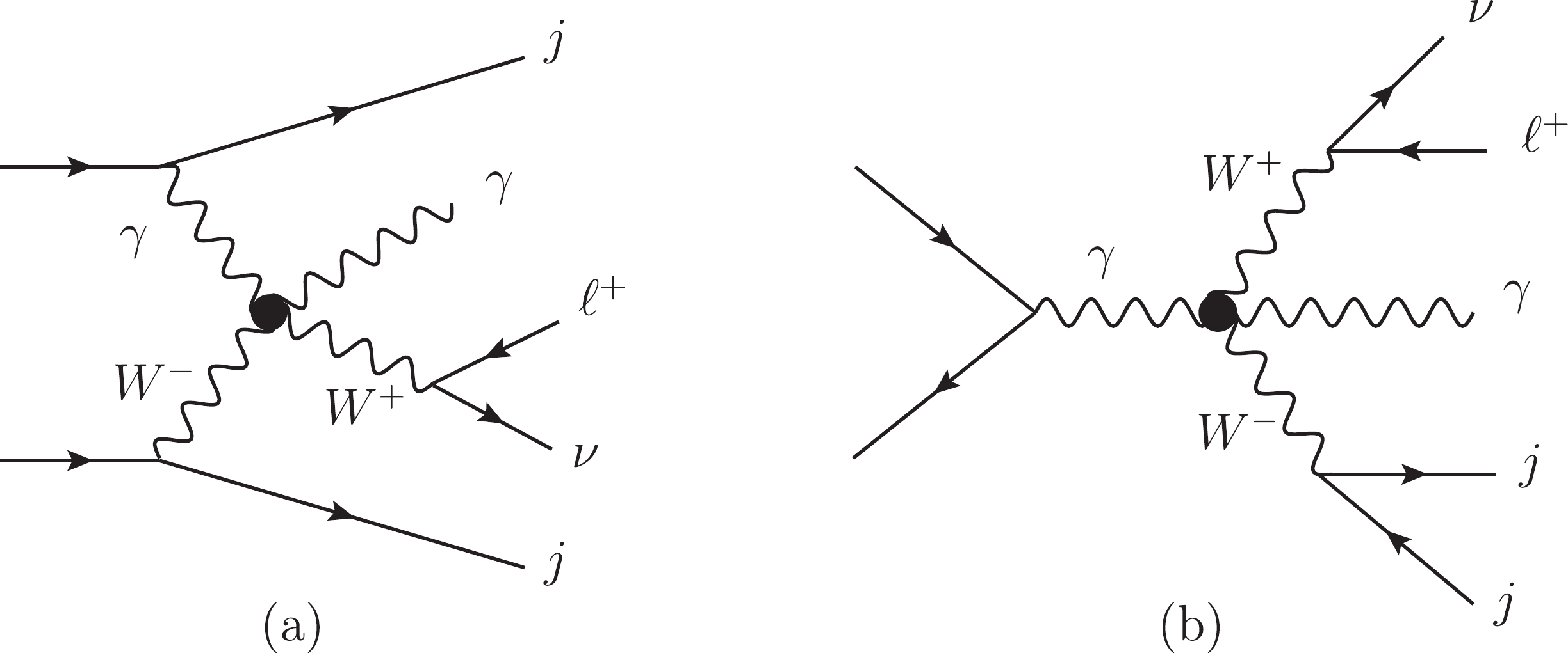

Figure 1.  Typical aQGC diagrams contributing to $\ell^+\nu\gamma jj$ final states. As in the SM, there are also VBS contributions as depicted in (a) and non-VBS contributions as in (b).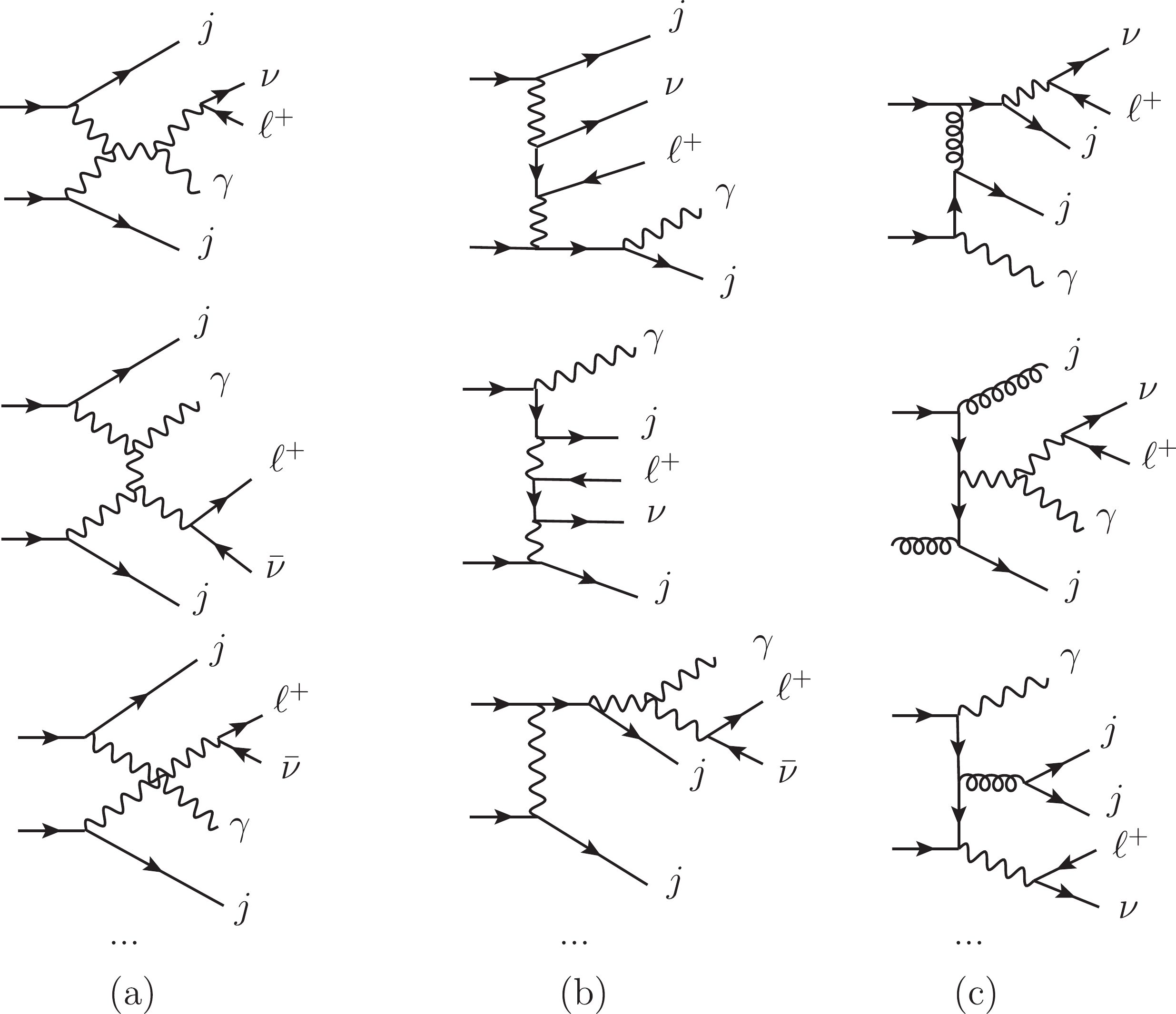

Figure 2.  Typical Feynman diagrams of SM backgrounds including (a) EW-VBS, (b) EW-non-VBS, and (c) QCD diagrams.

The numerical results are obtained through the Monte-Carlo (MC) simulation using the MadGraph5_aMC@NLO (MG5) toolkit [72]. The parton distribution function is NNPDF2.3 [73]. The renormalization scale $\mu_r$ and factorization scale $\mu_f$ are chosen to be dynamical and are set event-by-event as $\left(\prod _i^n \left(M_i^2+ {\vec p}_T^{(i)}\right)\right)^{\frac{1}{n}}$, with $i$ running over all heavy particles. The basic cuts are applied with the default settings of MG5 and require ${\vec p}_T^{\gamma,\ell}>10$ GeV, $|\eta _{\gamma,\ell}|>2.5$ and ${\vec p}_T^{j}>20$ GeV, $|\eta _j| < 5$. The events are then showered by PYTHIA8 [74] and a fast detector simulation is performed using Delphes [75] with the CMS detector card. Jets are clustered using the anti-$k_T$ algorithm with a cone radius $R = 0.5$ and $\vec{p}_{T,\min} = 20$ GeV. The photon isolation uses parameter $I_{\min}$ defined as [75]

where $\Delta R_{\max} = 0.5$and $\vec{p}_{T,\min} = 0.5$ GeV, and $I_{\min}^{\gamma} > 0.12$ . We generate the dominant signal events with the largest coefficients in Table 1. After fast detector simulation, the final states are not exactly $\ell ^+ \nu \gamma jj$. To ensure a high quality track of the signal candidate, a minimum number of composition is required. We denote the number of jets, photons, and charged leptons as $N_j$, $N_{\gamma}$, and $N_{\ell^+}$, respectively. Events are selected by requiring $N_j\geq 2$, $N_{\gamma}\geq 1$, and $N_{\ell^+} = 1$. We analyze the energy scale, kinematic features, and polarization features of the events after these particle number cuts.

Since the $O_{M_{0,1,7}}$ and $O_{T_{0,1,2}}$ operators are constrained tightly by $WWjj$, $WZjj$, and $ZZjj$ productions [61], we concentrate on the $O_{M_{2,3,4,5}}$ and $O_{T_{5,6,7}}$ operators.

To ensure that the events are generated by the EFT in a valid region, the unitarity bounds are applied as cuts on $\hat{s}$. However, $\hat{s}$ is not an observable because of the invisible neutrino. Instead, we find an observable to evaluate $\hat{s}$ approximately. We use the approximation that most of the $W$ bosons are on shell, such that $(p_{\ell}+p_{\nu})^2\approx M_W^2\ll \hat{s}$. Compared with a large $\hat{s}$, the mass of the $W$ boson is negligible; therefore, $2p_{\ell} p_{\nu}\approx 0$, which indicates that the flight direction of the neutrino is close to the charged lepton. We use an event selection strategy to select the events with a small azimuth angle between the charged lepton and the missing momentum, which is denoted as $\Delta \phi _{\ell m}$, to strengthen this approximation. The normalized distributions of $\cos (\Delta \phi _{\ell m})$ are depicted in Fig. 3(a). The distributions are similar for each class of operators (i.e., $O_{M_i}$ or $O_{T_i}$), but are different between $O_{M_i}$ and $O_{T_i}$. Therefore, we present only $O_{M_2}$ and $O_{T_5}$ as examples. We choose $\cos (\Delta \phi _{\ell m})>0.95$ to cut off the events with a small $\cos (\Delta \phi _{\ell m})$.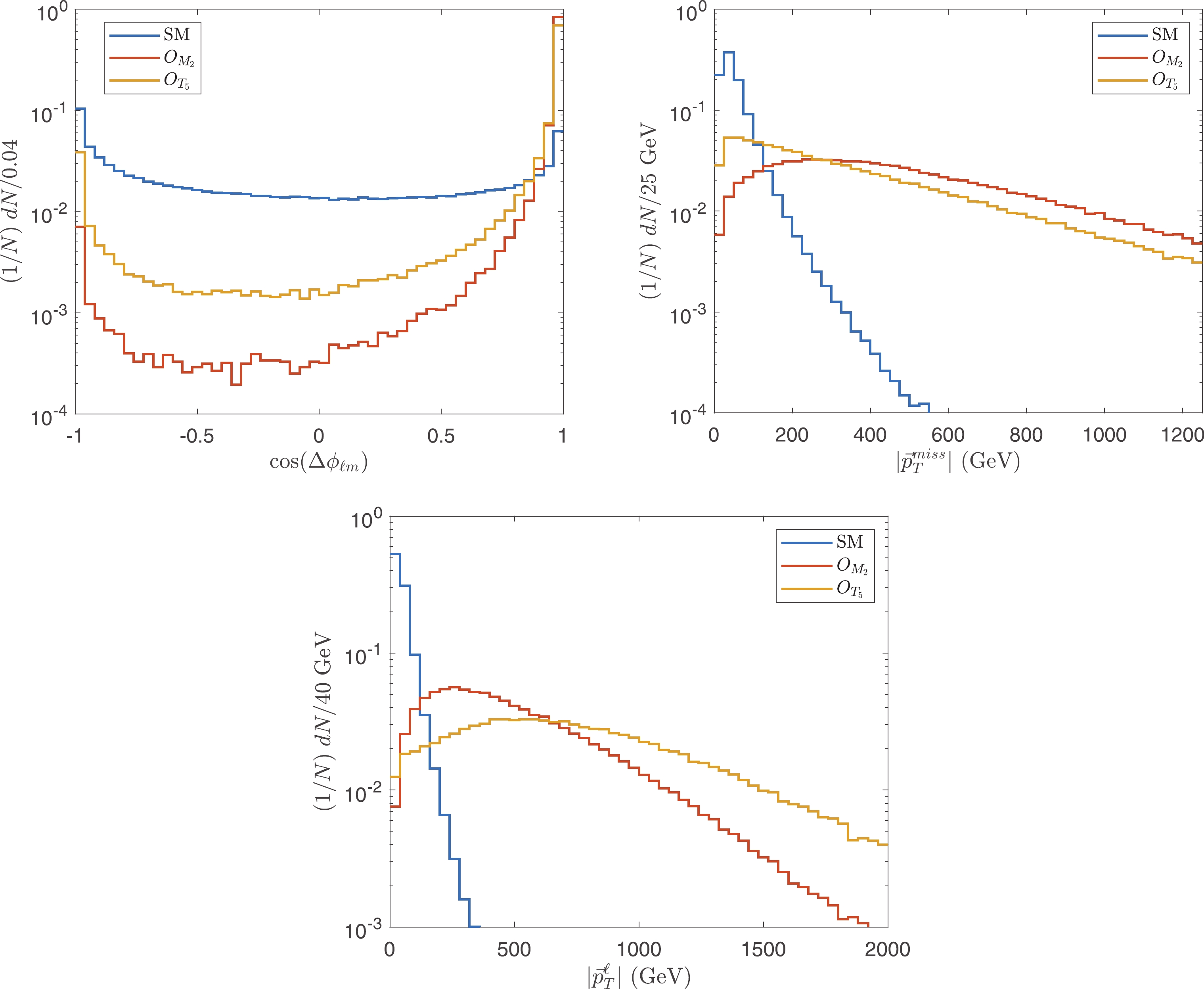

Figure 3.  (color online) Normalized distributions of $\cos (\Delta \phi _{\ell m})$, $|\vec{p}_T^{\rm miss}|$, and $|\vec{p}_T^{\ell}|$ after particle number cuts.

Using the approximation that the neutrino and charged lepton are nearly parallel to each other, and by also requiring $|{\vec p}^{\ell}_T|>0$, which is guaranteed due to the detector simulation, we introduce

where $E_{\ell,\gamma} = \sqrt{(p_x^{\ell,\gamma})^2+(p_y^{\ell,\gamma})^2+(p_z^{\ell,\gamma})^2}$, $\vec{p}_T^{\ell} = (p_x^{\ell},p_y^{\ell},0)$, $p_{x,y,z}^{\ell,\gamma}$ are components of the momenta of lepton and photon in the c.m. frame of $pp$, and $\vec{p}^{\rm miss}_T$ is the missing momentum. $\tilde{s}$ reconstructs $\hat{s}$ when the neutrino and charged lepton are exactly collinear and when the missing momentum is exactly neutrino transverse momentum. From the definition of $\tilde{s}$, one can see that, with a larger $|\vec{p}^{\ell}_T|$, the approximation is better. Meanwhile, the cross sections of the sub-processes $W^+\gamma\to W^+\gamma$ and $ZW^+\to W^+\gamma$ increase with $\sqrt{\hat{s}}$. Therefore, one can expect that the number of signal events increases with increasing $\hat{s}$, namely, one can expect an energetic $W^+$ boson. Therefore, the momentum of the charged lepton produced by the $W^+$ boson should also be large. For the same reason, $|\vec{p}_T^{\rm miss}|$ should also be large. A small $|\vec{p}_T^{\rm miss}|$ probably indicates a neutrino along the $\vec{z}$ direction. Approximation $\tilde{s}$ can benefit from cutting off such events. The normalized distributions of $|\vec{p}_T^{\ell}|$ and $|\vec{p}_T^{\rm miss}|$ after particle number cuts are shown in Fig. 3(b) and (c). We choose the events with $|\vec{p}_T^{\ell}|> 80\;{\rm{GeV}}$ and $|\vec{p}_T^{\rm miss}| > 50\;{\rm{GeV}}$.

To verify the approximation accuracy, we calculate both $\hat{s}$ and $\tilde{s}$. Unlike real experiments, in simulation, $\hat{s}$ can be obtained before detector simulation. Both $\hat{s}$ and $\tilde{s}$ are calculated after the $\Delta \phi _{\ell m}$, $|\vec{p}_T^{\ell}|$, and $|\vec{p}_T^{\rm miss}|$ cuts are applied. Consider $O_{M_2}$ and $O_{T_5}$ operators for example, as shown in Fig. 4. $\tilde{s}$ can approximate $\hat{s}$ well.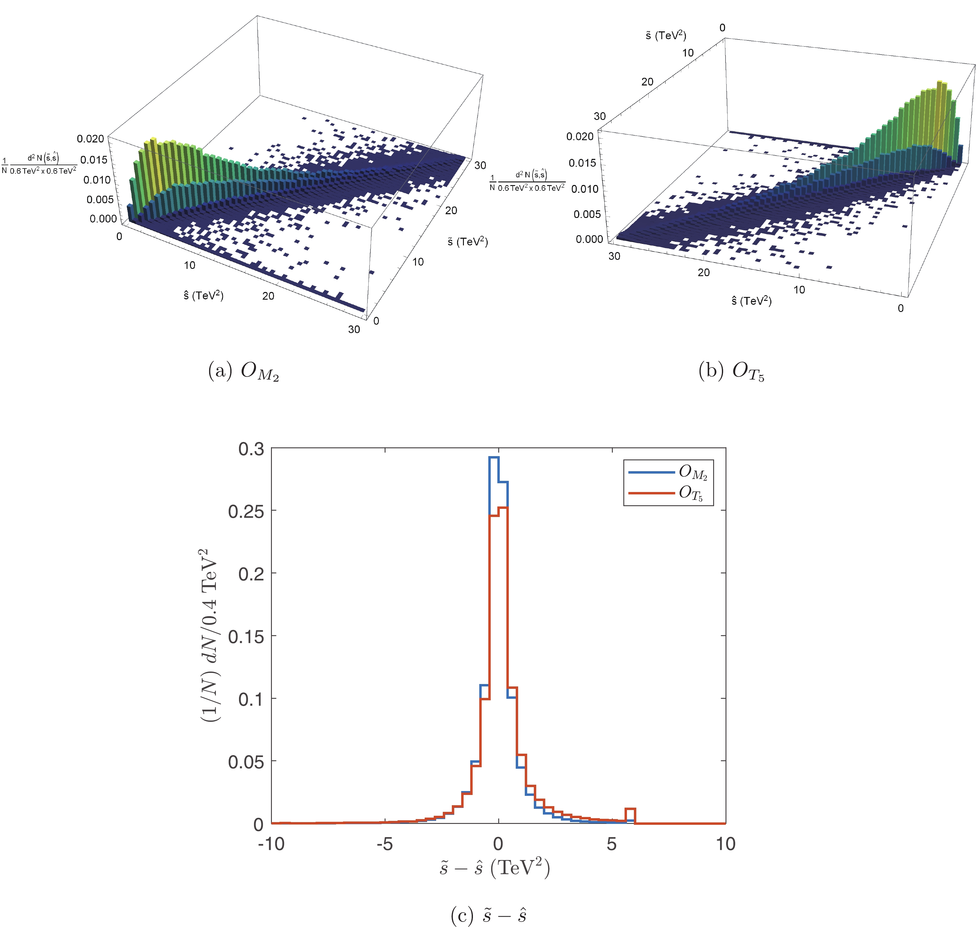

Figure 4.  (color online) Correlation between $\hat{s}$ and $\tilde{s}$ for $O_{M_2}$ and $O_{T_5}$.

The unitarity bounds are realized as energy cuts using $\tilde{s}$, denoted as $\tilde{s}_U$. From Eq. (14), the $\tilde{s}_U$ cuts are

The effects of the $\Delta \phi _{\ell m}$, $|\vec{p}_T^{\ell}|$, $|\vec{p}_T^{\rm miss}|$, and $\tilde{s}_U$ cuts are shown in Table 4. Theoretically, the unitarity bounds should not be applied to the SM backgrounds. However, in the aspect of the experiment, we cannot distinguish the aQGC signals from the SM backgrounds strictly. Thus, the $\tilde{s}_U$ cut can only be applied on all events. Therefore, we also apply the $\tilde{s}_U$ cuts on the SM backgrounds. We verify that the $\tilde{s}_U$ cuts have negligible effects on the SM backgrounds for all the largest $f_{M_{2,3,4,5}}/\Lambda^4$ and $f_{T_{5,6,7}}/\Lambda^4$ we are using.

Channel/fb	no cut	$N_{j,\gamma,\ell^+}$	$\Delta \phi _{\ell m}$	$|\vec{p}^{\ell}_T|$	$|\vec{p}_T^{\rm miss}|$	$\tilde{s}_U$
SM	$9520.8$	$3016.6$	$211.7$	$65.1$	$40.6$	−
$O_{M_2}$	$6.353$	$4.06$	$3.51$	$3.45$	$3.43$	$0.93$
$O_{M_3}$	$21.05$	$13.62$	$12.13$	$11.95$	$11.90$	$2.19$
$O_{M_4}$	$7.39$	$4.81$	$4.06$	$3.94$	$3.92$	$1.03$
$O_{M_5}$	$25.23$	$16.73$	$14.75$	$14.49$	$14.42$	$4.05$
$O_{T_5}$	$2.71$	$1.77$	$1.28$	$1.25$	$1.22$	$0.72$
$O_{T_6}$	$16.92$	$11.19$	$8.94$	$8.36$	$8.26$	$3.06$
$O_{T_7}$	$7.47$	$4.97$	$3.97$	$3.69$	$3.65$	$1.43$

Table 4.  Cross sections of SM backgrounds and signals for various operators after $N_{j,\gamma,\ell^+}$, $\Delta \phi _{\ell m}$, $|\vec{p}^{\ell}_T|$, $|\vec{p}_T^{\rm miss}|$, and $\tilde{s}_U$ cuts. The maximum $\tilde{s}$ used in the $\tilde{s}_U$ cuts are obtained using the upper bounds of $f_X/\Lambda ^4$ in Table 1 and Eq. (17).

From Table 4, it is evident that the unitarity bounds have significant suppressive impacts on the signals, particularly for the $O_{M_i}$ operators, indicating the necessity of the unitarity bounds.

As already mentioned, the VBS processes do not increase with $\sqrt{\hat{s}}$in the SM. This opens a window to detect aQGCs. To focus on the VBS contributions, we investigate the efficiencies of the standard VBS/VBF cuts [21]. The VBS/VBF cuts are designed to highlight the VBS contributions from the SM and BSM; however, they cannot cut off the SM VBS contributions. Therefore, they are not as efficient as other cuts designed for aQGCs only. We impose only$|\Delta y_{jj}|$, which is defined as the difference between the pseudo rapidities of the two hardest jets. The normalized distributions of $|\Delta y_{jj}|$ are depicted in Fig. 5(a). It is evident that $|\Delta y_{jj}|$ is an efficient cut for the $O_{M_i}$ operators, and we select the events with $|\Delta y_{jj}| > 1.5$.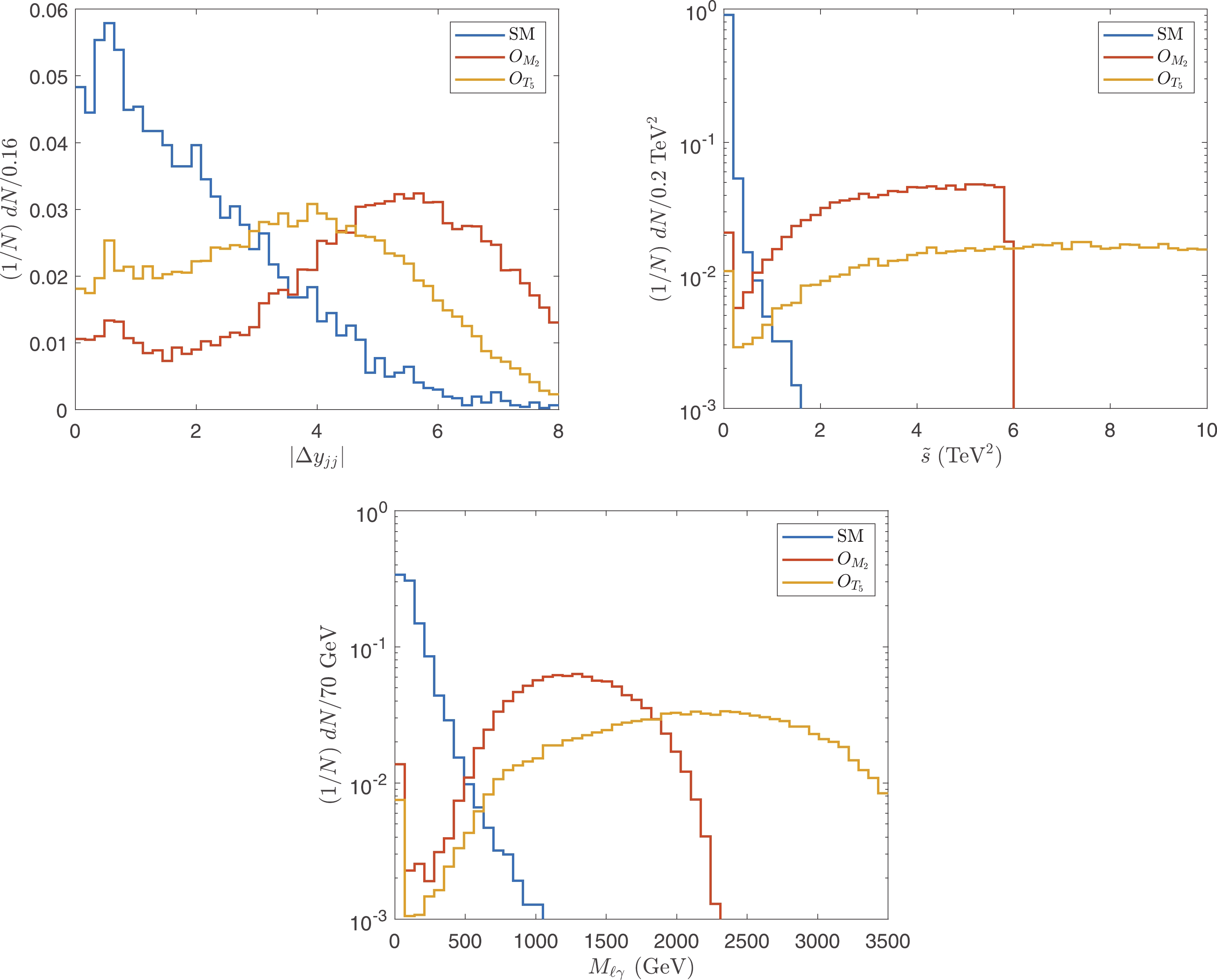

Figure 5.  (color online) Normalized distributions of $|\Delta y_{jj}|$, $\tilde{s}$, and $M_{\ell\gamma}$ after $\tilde{s}_U$ cut.

For the lepton and photon, the cuts are mainly to select events with large $\hat{s}$. The normalized distributions of $\tilde{s}$ are shown in Fig. 5(b). We select the events with $\tilde{s}> 0.4$ ${\rm TeV}^2$. To distinguish from the $\tilde{s}_U$ cut, $\tilde{s}$ cut in this subsection is denoted as $\tilde{s}^{\rm{cut}}$.

There are other sensitive observables to select large $\hat{s}$ events, such as the invariant mass of the charged lepton and photon defined as $M_{\ell \gamma} = \sqrt{(p_{\ell}+p_{\gamma})^2}$, and the angle between the photon and charged lepton. We find that, after the $\tilde{s}^{\rm{cut}}$ cut, the other cuts are redundant. Consider $M_{\ell \gamma}$ as an example. The normalized distributions of $M_{\ell \gamma}$ are shown in Fig. 5(c). As shown, $M_{\ell \gamma}$ is a significantly sensitive observable, and $M_{\ell \gamma} > {M^{\rm{cut}}_{\ell \gamma}}$ can be used as an efficient cut. However, note that after $\tilde{s}^{\rm{cut}}$, due to $M_{\ell \gamma}\leq \sqrt{\tilde{s}}$, one must choose a significantly large ${M^{\rm{cut}}_{\ell \gamma}}$, which is almost equivalent to a large $\tilde{s}^{\rm{cut}}$.

To improve the event select strategy, we investigate the polarization features that are less correlated with $\tilde{s}$. As is evident from Tables 2 and 3, for $O_{M_i}$, the leading contributions of the signals are those with longitudinal $W^+$ bosons in the final states, whereas for $O_{T_i}$, both the left- and right-handed $W^+$ bosons dominate. The polarization of the $W^+$ boson can be inferred by the momentum of the charged lepton in the $W^+$ boson rest-frame, the so called helicity frame, as [76]

where $\theta^*$ is the angle between the flight directions of $\ell^+$ and $W^+$ in the helicity frame;$f_L$, $f_R$, and $f_0 = 1-f_L-f_R$ are the fractions of the left-handed, right-handed, and longitudinal polarizations, respectively. Because the neutrinos are invisible, it is difficult to reconstruct the momentum of the $W^+$ boson and boost the lepton to the rest frame of the $W^+$ boson. However, when the transverse momentum of the $W^+$ boson is large, $\cos (\theta ^*)$ can be obtained approximately as $\cos (\theta ^*) \approx 2(L_p - 1)$ with $L_p$ defined as [58]

where $\vec{p}_T^W = \vec{p}_T^{\ell}+\vec{p}_T^{\rm miss}$. For the signal events of the $O_{M_i}$ or $O_{T_i}$ operators, the polarization fractions of the$W^+$ bosons are different from those in the SM backgrounds. The polarization fractions can be categorized into four patterns: the SM, $O_{M_i}$, $O_{T_{0,5}}$, and$O_{T_{1,2,6,7}}$ patterns. $O_{M_2}$, $O_{T_5}$, and $O_{T_7}$ are chosen as the representations. Neglecting the events with $L_p\notin [0, 1]$, the normalized distributions of $L_p$ after $\tilde{s}_U$ cuts are depicted in Fig. 6.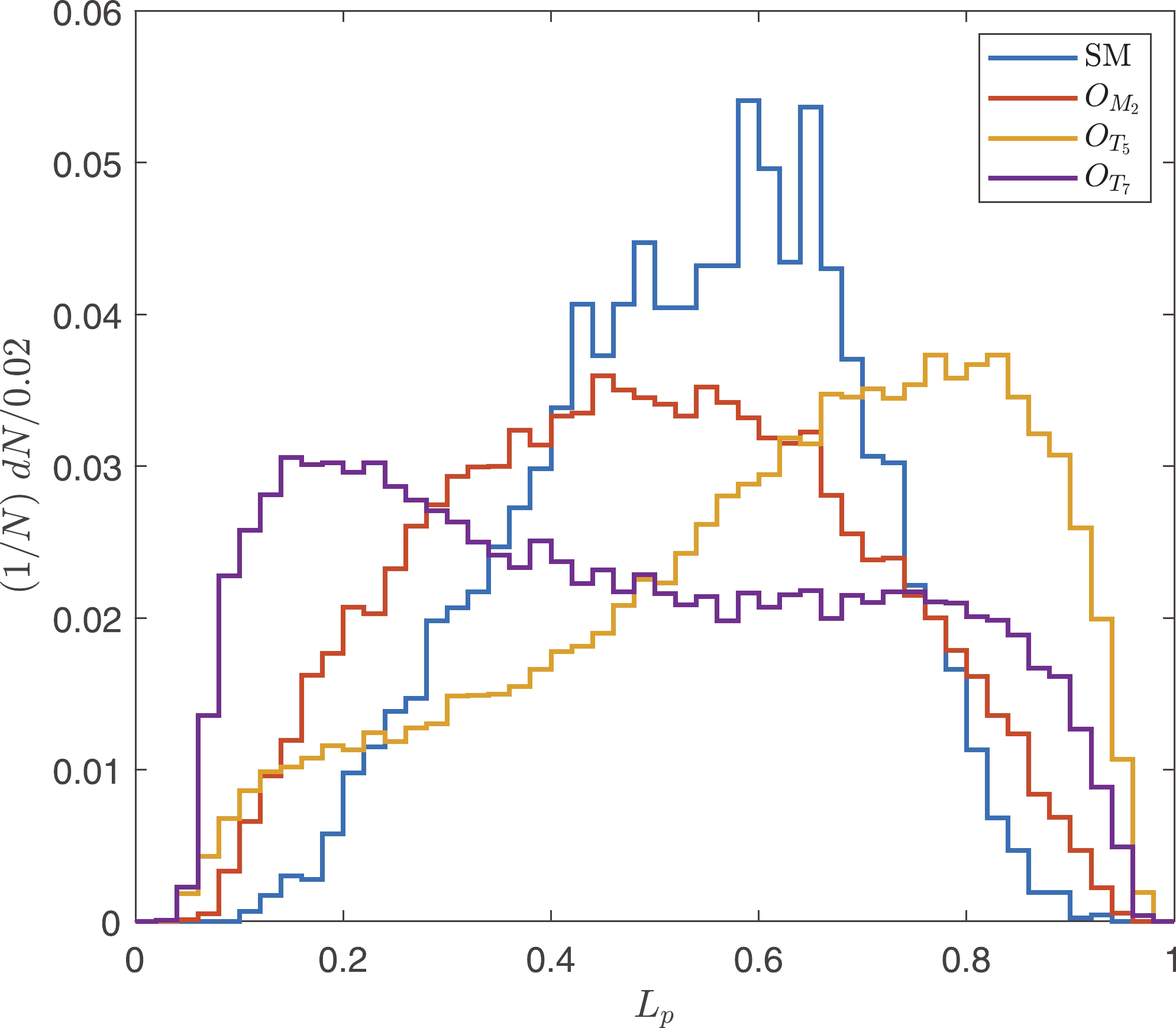

Figure 6.  (color online) Normalized distributions of $L_p$.

As presented in Tables 2 and 3, the polarization of the $W^+$ boson is related to $\theta$, which is the angle between the outgoing photon and the $\vec{z}$-axis of the c.m. frame of the sub-process; however, $\theta$ is not an observable. Because the protons are energetic, we assume that the vector bosons in the initial states of the sub-processes carry large fractions of proton momenta. Therefore, their flight directions are close to the protons in the c.m. frame. In this way, $\theta$ could be approximately estimated using the angle between outgoing photons and the $\vec{z}$-axis of the c.m. frame of protons, which is denoted as $\theta '$. The correlation features between $\theta '$ and $L_p$ can be used to extract the aQGC signal events from the SM backgrounds. The correlations of $\theta'$ and $L_p$ for the SM, and for the $O_{M_2}$, $O_{T_5}$, and $O_{T_7}$ operators are established in Fig. 7. From Fig. 7, it is evident that signal events of $O_{T_{5,7}}$ distribute differently from the SM backgrounds. The distribution for the SM peaks at $|\cos(\theta ')|\approx 1$ and $L_p\approx 0.5$, the distribution for $O_{T_5}$ peaks at $|\cos(\theta ')|\approx 1$ and $L_p\approx 0$, and the distribution for $O_{T_7}$ peaks at $|\cos(\theta ')|\approx 1$ and $L_p\approx 1$. Therefore, we define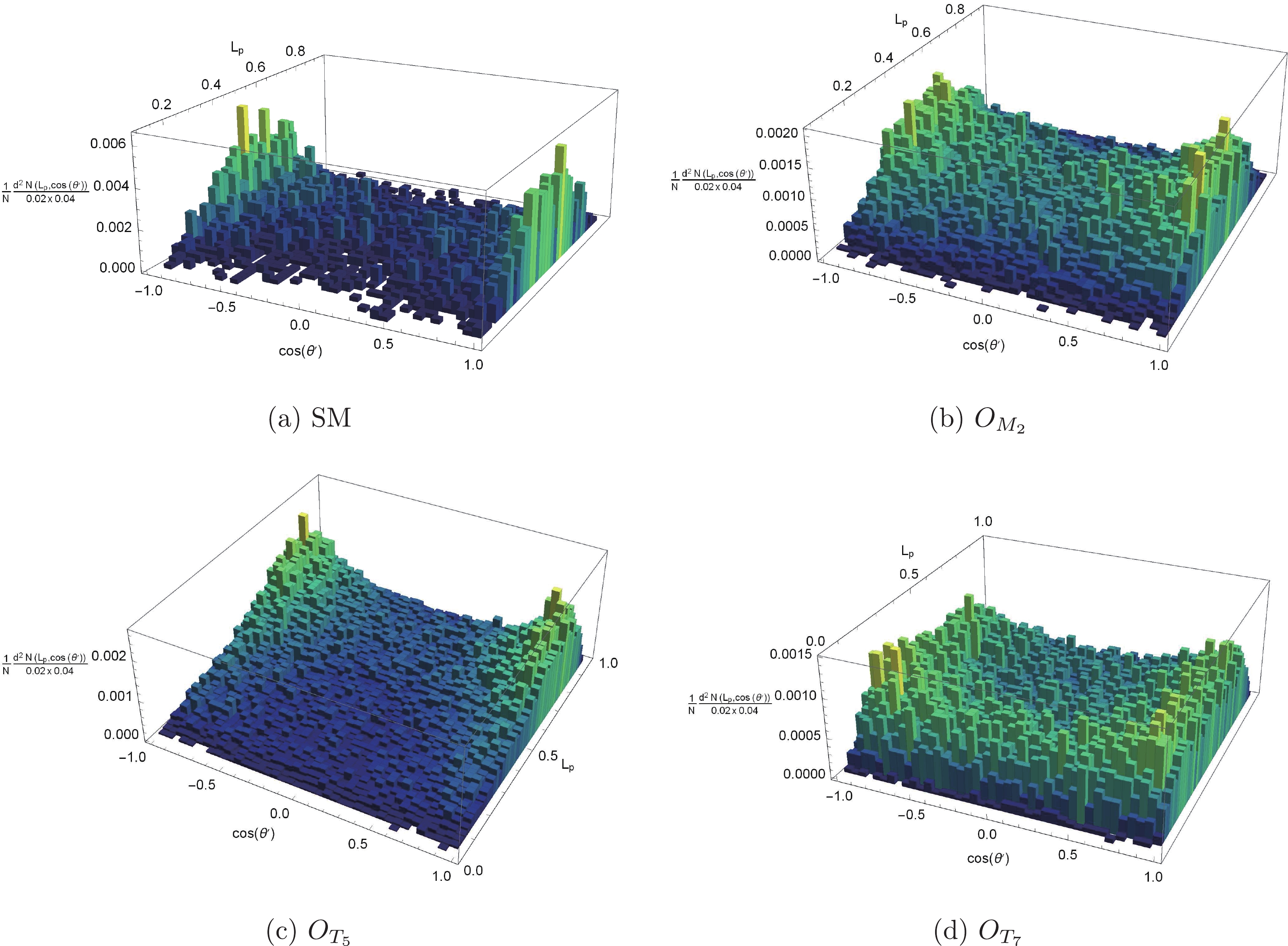

Figure 7.  (color online) Normalized distributions of $L_p$ and $\cos \theta '$. Each bin corresponds to ${\rm d} L_p \times {\rm d} \left(\cos \theta'\right) = 0.02\times 0.04$ ($50\times 50$ bins).

where $r$ is a sensitive observable that can be used as a cut to discriminate the signals of the $O_{T_{5,6,7}}$ operators from the SM backgrounds. The normalized distributions are shown in Fig. 8. We select the events with $r>0.05$.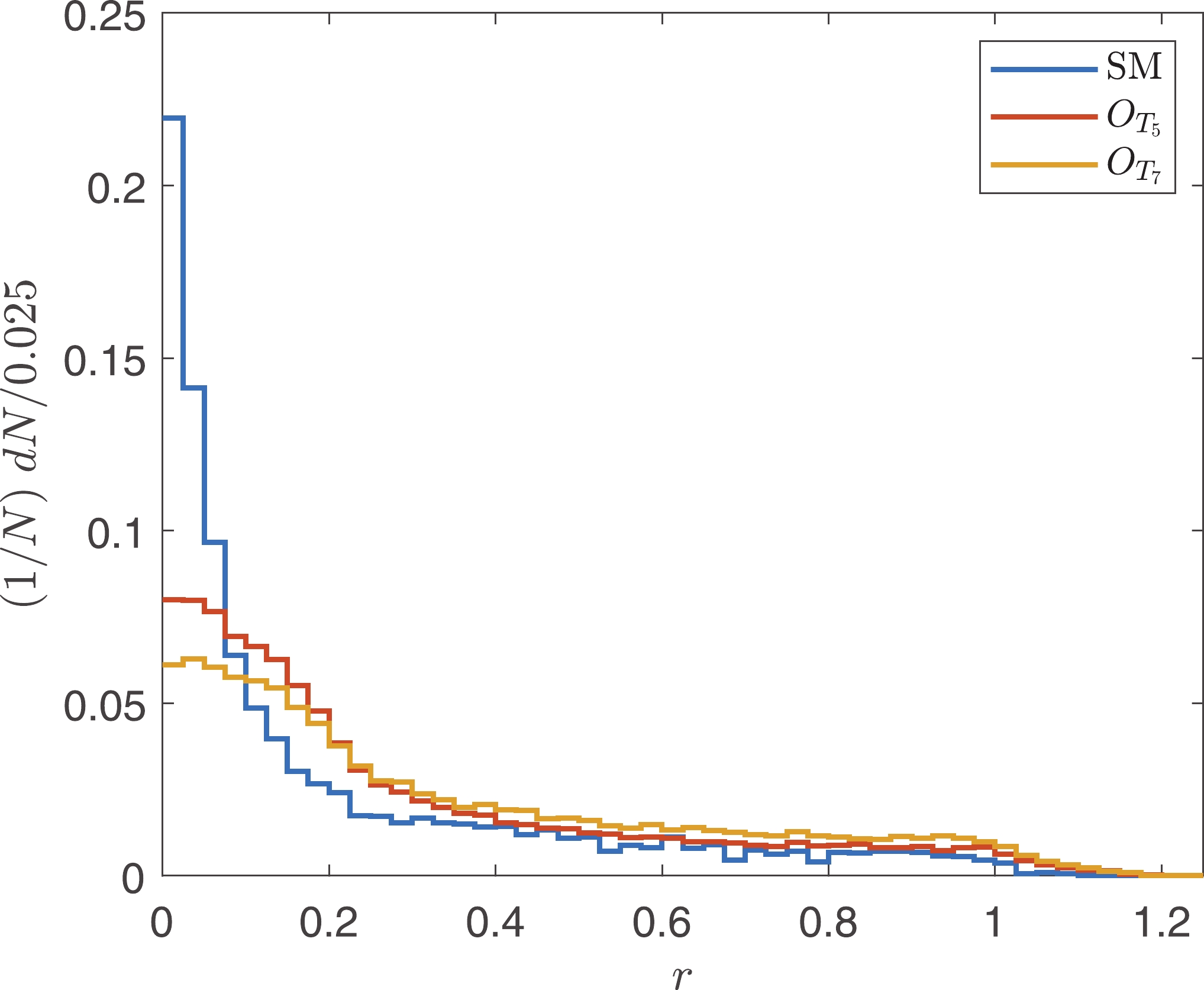

Figure 8.  (color online) Normalized distributions of $r$ after $\tilde{s}_U$ cut.

To verify that $r$ cut is not redundant, we calculate the correlation between $\tilde{s}$ and $M_{\ell \gamma}$, and compare it with the correlation between $\tilde{s}$ and $r$. Consider the SM backgrounds and the signal of $O_{T_5}$ as examples. The results are shown in Fig. 9. It is evident that the events with small $M_{\ell \gamma}$ are almost those with small $\tilde{s}$; however, the same is not the case for $r$.

Figure 9.  (color online) Correlations between $M_{\ell\gamma}$ and $\tilde{s}$ (upper panels), $r$ and $\tilde{s}$ (bottom panels) for $O_{T_5}$, and the SM backgrounds.

For various operators, the kinematic and polarization features are different. Therefore, we propose to use various cuts to search for different operators, as summarized in Table 5. Note that $\tilde{s}^{\rm{cut}}$ in fact also cut off all the events with small $M_{\ell\gamma}$. Therefore, $\left|M_{\ell\gamma}-M_Z\right| >10\;{\rm{GeV}}$ is satisfied. The latter is used to reduce the backgrounds from $Z\to \ell\ell$ with one $\ell$ mis-tagged as a photon in the previous study of $W\gamma jj$ production [39], and $\tilde{s}^{\rm{cut}}$ has a similar effect.

$O_{M_i}$	$O_{T_{5,6,7}}$
$\tilde{s}>0.4 \; {{\rm{TeV}}}^2$	$\tilde{s}>0.4 \; {{\rm{TeV}}}^2$
$|\Delta y_{jj}|>1.5$	$0\leqslant L_p\leqslant 1$, $r>0.05$

Table 5.  Two classes of cuts.

The results are shown in Table 6. The statistical error is negligible compared with the systematic error; therefore, it is not presented. The large SM backgrounds can be reduced effectively using our selection strategy.

Channel	after $\tilde{s}_U$	after $\tilde{s}^{\rm{cut}}$	$|\Delta y_{jj}|$ or $r$
SM	$40.6$	$1.70$	$0.93^{+0.23}_{-0.17}$ ($\Delta y_{jj}$)
			$1.05^{+0.26}_{-0.19}$ ($r$)
$O_{M_2}$	$0.93$	$0.91$	$0.82^{+0.20}_{-0.15}$
$O_{M_3}$	$2.19$	$2.11$	$1.90^{+0.48}_{-0.35}$
$O_{M_4}$	$1.03$	$1.01$	$0.91^{+0.23}_{-0.16}$
$O_{M_5}$	$4.05$	$3.94$	$3.55^{+0.89}_{-0.64}$
$O_{T_5}$	$0.72$	$0.71$	$0.60^{+0.15}_{-0.11}$
$O_{T_6}$	$3.06$	$3.01$	$2.69^{+0.62}_{-0.48}$
$O_{T_7}$	$1.43$	$1.40$	$1.12^{+0.28}_{-0.20}$

Table 6.  Cross sections (fb) of signals and SM backgrounds after $\tilde{s}^{\rm{cut}}$, $|\Delta y_{jj}|$, and $r$ cuts. The column "After $\tilde{s}_U$" is the same as the last column in Table 4.

To investigate the signals of aQGCs, one should investigate how the cross section is modified by adding dimension-8 operators to the SM Lagrangian. Furthermore, the effect of interference is also included. In this section, we investigate the process $pp\to \ell^+ \nu \gamma j j$ with all Feynman diagrams including non-VBS aQGC diagrams, such as Fig. 1(b), and with all possible interference effects.

To investigate the parameter space, we generate events with each operator individually. The unitarity bounds are set as $\tilde{s}_U$ cuts, which depend on $f_{M_i}/\Lambda ^4$ and $f_{T_i}/\Lambda ^4$ used to generate the events. The cross sections as functions of $f_{M_i}/\Lambda ^4$ and $f_{T_i}/\Lambda ^4$ are shown in Figs. 10 and 11. The results with and without the unitarity bounds are presented. As is evident from Figs. 10 and 11, the cross sections are approximately bilinear functions of $f_{M_i}/\Lambda ^4$ and $f_{T_i}/\Lambda ^4$without the unitarity bounds. However, the unitarity bounds significantly suppress the signals, and the resulting cross sections are no longer bilinear functions. From Figs. 10 and 11, it is also evident that the $W\gamma jj$ production is more sensitive to the $O_{M_{3,5}}$ and $O_{T_{6,7}}$ operators.

Figure 10.  (color online) Cross sections as functions of $f_{M_i/\Lambda^4}$ with and without unitarity bounds.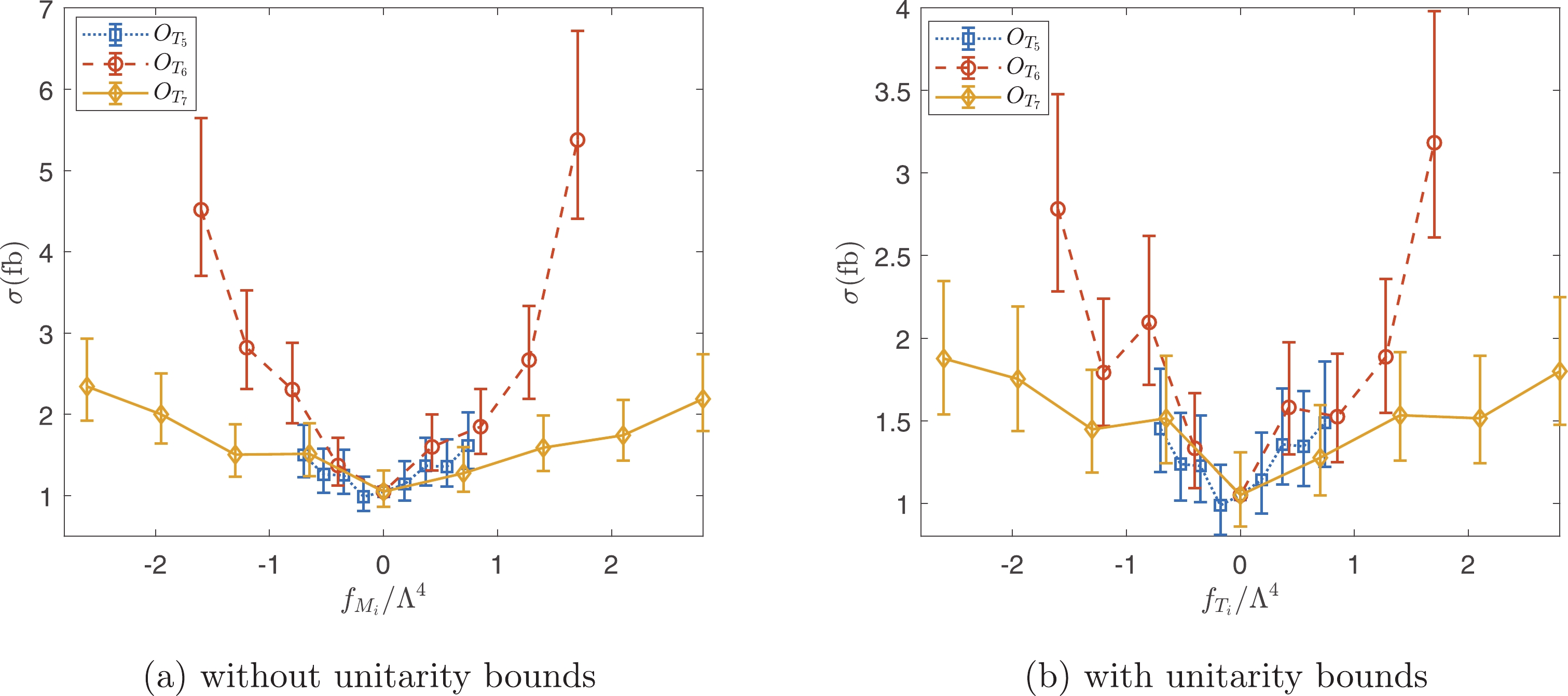

Figure 11.  (color online) Cross sections as functions of $f_{T_i/\Lambda^4}$ with and without unitarity bounds.

The constraints on operator coefficients can be estimated with the help of statistical significance defined as ${\cal{S}}_{\rm stat}\equiv N_S/\sqrt{N_S+N_B}$, where $N_S$ is the number of signal events and $N_B$ is the number of the background events. The total luminosity, ${\cal{L}}$, at $13\;{{\rm{TeV}}}$ for the years 2016, 2017, and 2018 is ${\cal{L}}\approx 137.1\;{{\rm{fb}}^{-1}}$ [77]. For each $f_X/\Lambda ^4$ used to generate the events, the $\tilde{s}_U$ cut can be set accordingly; subsequently, ${\cal{S}}_{\rm stat}$ at $137.1\;{{\rm{fb}}^{-1}}$ and $13\;{{\rm{TeV}}}$ can be obtained. The constraints are set by the lowest positive $f_X/\Lambda ^4$ and the greatest negative $f_X/\Lambda ^4$ with ${\cal{S}}_{\rm stat}$ larger than the required statistical significance. The constraints on the coefficients at current luminosity are depicted in Table 7. Comparing the constraints from 13 TeV CMS experiments in Table 1 with the ones in Table 7, it is evident that, even with the unitarity bounds suppressing the signals, the allowed parameter space can still be reduced significantly using our efficient event selection strategy.

Coefficients	${\cal{S} }_{\rm stat} > 2$		Coefficients	${\cal{S} }_{\rm stat} > 2$
$f_{M_2}/\Lambda ^4$	$[-2.05, 2.0]$		$f_{T_5}/\Lambda ^4$	$[-0.525, 0.37]$
$f_{M_3}/\Lambda ^4$	$[-10.5, 5.25]$		$f_{T_6}/\Lambda ^4$	$[-0.4, 0.425]$
$f_{M_4}/\Lambda ^4$	$[-11.25, 4.0]$		$f_{T_7}/\Lambda ^4$	$[-0.65, 0.7]$
$f_{M_5}/\Lambda ^4$	$[-6.25, 6.0]$

Table 7.  Constraints on operators at LHC with ${\cal{L}} = 137.1\; {{\rm{fb}}^{-1}}$.

The accurate measurement of VBS processes at the LHC is very important for the understanding of the SM and search of BSM. In recent years, the VBS processes have received significant attention and been studied extensively. To investigate the signals of BSM, a model independent approach, known as the SMEFT, is used frequently. The effects of BSM show up as higher dimensional operators. The VBS processes can be used to probe dimension-8 anomalous quartic gauge-boson operators. In this study, we focused on the effects of aQGCs in the $pp\to W \gamma jj$process. The operators concerned are summarized, and the corresponding vertices are obtained.

An important consideration regarding the SMEFT is that of its validity. We studied the validity of the SMEFT using the partial-wave unitarity bound, which sets an upper bound on $\hat{s}^2 |f_X|$, where $f_X$ is the coefficient of operator $O_X$. In other words, there exists a maximum $\hat{s}$ for a fixed coefficient in the sense of unitarity. We discard all the events with $\hat{s}$ larger than the maximally allowed one, so that the results obtained via the SMEFT are guaranteed to respect unitarity. For this purpose, we find an observable that can approximate $\hat{s}$ very well, denoted as $\tilde{s}$, based on which the unitarity bounds are applied. Due to the fact that there are massive $W^+$ or/and $Z$ bosons in the initial state of the sub-process, and that the massive particle emitting from a proton can carry a large fraction of the proton momentum, the c.m. energy of the sub-process is found to be of the same order as the c.m. energy of the corresponding process. As a consequence, at large c.m. energy, the unitarity bounds are very strict, and the cuts can significantly reduce the signals.

To study the discovery potential of aQGCs, we investigate the kinematic features of the signals induced by aQGCs and find that $\tilde{s}$ serves as a very efficient cut to highlight the signals. We also find that other cuts to cut off the events with small $\hat{s}$ are redundant. To find other sensitive observables less correlated with $\hat{s}$, we investigate the polarization features of the signals. The polarization features of $O_{T_i}$ operators are found to be very different from the SM backgrounds. We find a sensitive observable $r$ to select the signal events of the $O_{T_i}$ operators. Although the signals of aQGCs are highly suppressed by unitarity bounds, the constraints on the coefficients for the $O_{M_{2,3,4,5}}$ and $O_{T_{5,6,7}}$ operators can still be tightened significantly with current luminosity at 13 TeV LHC.

We thank Jian Wang and Cen Zhang for useful discussions.