


 Abstract
 HTML
HTML Reference
 Related
 PDF
PDF


-
Recently, double-beauty tetraquarks, composed of a
$ bb $ diquark and a light antidiquark$ \overline{q}\overline{q}^{\prime } $ , became a subject of intensive theoretical studies [1-6]. The interest in these states was inspired by the experimental observation of baryons$ \Xi _{cc}^{++} $ and measurements of their parameters [7]. The measurements were used in phenomenological models, to estimate the masses of double-beauty states [1]. These investigations demonstrated that the axial-vector tetraquark$ T_{bb;\overline{u}\overline{d}}^{-} $ (hereafter$ T_{bb}^{-} $ ) with the mass$ m = (10389\pm 12)\; \mathrm{MeV} $ is stable with respect to strong and electromagnetic decays and can dissociate into a conventional meson only via a weak transformation. A similar conclusion about the stable nature of some tetraquarks$ bb\overline{q}\overline{q}^{\prime } $ was reached in Ref. [2] as well, where the authors of that study used methods of heavy-quark symmetry analysis.Double-heavy tetraquarks
$ QQ^{\prime }\overline{q}\overline{q}^{\prime } $ , in fairness, were studied already in classical articles [8-12], in which they were examined as candidate stable four-quark compounds. The main qualitative conclusion drawn in these works was the existence of a constraint on the masses of constituent quarks. It was found that tetraquarks$ QQ^{\prime }\overline{q}\overline{q}^{\prime } $ may form strong-interaction stable exotic mesons, provided the ratio$ m_{Q}/m_{q} $ is large. Therefore, tetraquarks$ bb \overline{q}\overline{q}^{\prime } $ are the most promising candidates for stable four-quark mesons.Quantitative analysis of these problems continued in the following years, using the frameworks of various models and using different methods from high-energy physics. Thus, tetraquarks
$ T_{QQ} $ were explored using the chiral, dynamical, and relativistic quark models [13-17]. Axial-vector states$ T_{QQ;\overline{u}\overline{d}} $ were considered in the context of the sum rule method [18,19]. Processes in which tetraquarks$ T_{cc} $ may be produced, namely electron-positron annihilation, heavy-ion and proton-proton collisions, and$ B_{c} $ meson and$ \Xi _{bc} $ baryon decays, also attracted the interest of researchers [20-24].The axial-vector particle
$ T_{bb}^{-} $ was studied in our work as well [3]. We employed the quantum chromodynamics (QCD) sum rule method and evaluated the mass of this state$ m = (10035\; \pm 260)\; \mathrm{MeV} $ . This means that m is below both the$ B^{-}\overline{B}^{\ast 0} $ and$ B^{-}\overline{B}^{0}\gamma $ thresholds; hence, this state is a strong- and electromagnetic-interaction stable tetraquark. We also explored the semileptonic decays$ T_{bb}^{-} $ $ \rightarrow Z_{bc}^{0}l\overline{\nu }_{l} $ , where$ Z_{bc}^{0} $ is the scalar tetraquark$ [bc][\overline{u}\overline{d}] $ composed of color-triplet diquarks, and calculated their partial widths. The predictions for the full width and mean lifetime of$ T_{bb}^{-} $ obtained in Ref. [3] are useful for experimental investigations of double-beauty exotic mesons.Other members of the
$ bb\overline{q}\overline{q}^{\prime } $ family, studied in a rather detailed form, are the scalar tetraquarks$ T_{bb;\overline{u} \overline{s}}^{-} $ and$ T_{bb;\overline{u}\overline{d}}^{-} $ (in short forms,$ T_{b:\overline{s}}^{-} $ and$ T_{b:\overline{d}}^{-} $ , respectively). The mass and coupling of$ T_{b:\overline{s}}^{-} $ and$ T_{b:\overline{d}}^{-} $ were calculated in Refs. [25,26], in which we demonstrated that they cannot decay to ordinary mesons through strong and electromagnetic processes. We also investigated dominant semileptonic and nonleptonic weak decays of these tetraquarks and estimated their full width and lifetime characteristics.In the present article, we extend our analysis and investigate the axial-vector partner of
$ T_{b:\overline{s}}^{-} $ with the same quark content$ bb\overline{u}\overline{s} $ . It can be treated also as "s" member of the axial-vector multiplet of the states$ bb\overline{u}\overline{q} $ . We denote this tetraquark as$ T_{b:\overline{s}}^{\mathrm{AV}} $ and compute its spectroscopic parameters using the two-point QCD sum rule method. Calculations are performed by taking into account various vacuum condensates, up to 10 dimensions. The obtained result for its mass$ m = (10215\pm 250)\; \mathrm{MeV} $ proves that this state is stable against strong and electromagnetic decays. In fact,$ T_{b:\overline{s}}^{\mathrm{AV}} $ in the S-wave can decompose into pairs of conventional mesons$ B^{-}B_{s}^{\ast } $ and$ B^{\ast -}\overline{B}_{s}^{0} $ , provided m exceeds the corresponding thresholds$ 10695/ 10692\; \mathrm{MeV} $ , respectively. The threshold for the electromagnetic decay to the final state$ B^{-}\overline{B}_{s}^{0}\gamma $ is$ 10646\; \mathrm{MeV} $ . It is seen that even the maximal allowed value of the mass$ 10465\; \mathrm{MeV} $ is below all of these limits.Therefore, to evaluate the full width and lifetime of
$ T_{b:\overline{s}}^{\mathrm{AV}} $ , we analyzed the semileptonic and nonleptonic weak decays$ T_{b:\overline{s}}^{\mathrm{AV}}\rightarrow {\cal{Z}}_{b:\overline{s}}^{0}l \overline{\nu }_{l} $ and$ T_{b:\overline{s}}^{\mathrm{AV}}\rightarrow {\cal{Z}}_{b:\overline{s}}^{0}M $ , respectively. Here,$ {\cal{Z}}_{b:\overline{s}}^{0} $ is the scalar tetraquark$ [bc][\overline{u}\overline{s}] $ built of a color-triplet diquark and an antidiquark, and M is one of the vector mesons$ \rho ^{-} $ ,$ K^{\ast }(892) $ ,$ \ D^{\ast }(2010)^{-} $ , and$ \ D_{s}^{\ast -} $ . The weak transitions of$ T_{b:\overline{s}}^{\mathrm{AV}} $ can be described by the form factors$ G_{i}(q^{2}) $ ($ i = 0,1,2,3 $ ), which determine the differential rates${\rm d}\Gamma /{\rm d}q^{2}$ of the semileptonic and partial widths of the nonleptonic processes. These weak form factors are extracted from the QCD three-point sum rules in Section III.This work is structured as follows. In Section II, we calculate the mass and coupling of the tetraquarks
$ T_{b:\overline{s}}^{\mathrm{AV}} $ and$ {\cal{Z}}_{b:\overline{s}}^{0} $ . For this, we derive the sum rules for their masses and couplings, by analyzing the corresponding two-point correlation functions. Numerical computations are performed by taking into account quark, gluon, and mixed condensates, up to the 10th dimension. In Section III, we compute the weak form factors$ G_{i}(q^{2}) $ from the three-point sum rules for momentum transfers$ q^{2} $ , where this method is applicable. In that section, we also determine model functions$ {\cal{G}}_{i}(q^{2}) $ and find the partial widths of the semileptonic decays$ T_{b:\overline{s}}^{\mathrm{AV}}\rightarrow {\cal{Z}}_{b:\overline{s}}^{0}l\overline{\nu }_{l} $ . The weak nonleptonic processes$ T_{b:\overline{s}}^{\mathrm{AV}}\rightarrow {\cal{Z}}_{b:\overline{s}}^{0}M $ are investigated in Section IV. This section also contains our final results for the full width and mean lifetime of the tetraquark$ T_{b:\overline{s}}^{\mathrm{AV}} $ . In Section V we discuss our obtained results and present our conclusions. Appendix contains explicit expressions of quark propagators and the correlation function used to evaluate the parameters of the tetraquark$ T_{b:\overline{s}}^{\mathrm{AV}} $ . -
In this section, we calculate the mass
$ m_{\mathrm{AV}} $ and coupling$ f_{\mathrm{AV}} $ of the axial-vector tetraquark$ T_{b:\overline{s}}^{\mathrm{AV}} $ , which is necessary for clarifying its nature, and conclude whether this particle is stable against strong and electromagnetic decays. Another tetraquark considered here is the scalar exotic meson$ {\cal{Z}}_{b:\overline{s}}^{0} $ that appears in the final state of the master particle's decays: spectroscopic parameters of this state enter into the expressions for the partial widths of the$ T_{b:\overline{s}}^{\mathrm{AV}} $ tetraquark's decay channels. The scalar exotic meson$ {\cal{Z}}_{b:\overline{s}}^{0} $ is a member of the$ bc\overline{q}\overline{q}^{\prime } $ family and is of interest from this perspective as well.The sum rules for evaluating the mass and coupling of the axial-vector tetraquark
$ T_{b:\overline{s}}^{\mathrm{AV}} $ can be obtained from the two-point correlation function$ \begin{array}{l} \Pi _{\mu \nu }(p) = {\rm i}\displaystyle\int {\rm d}^{4}x{\rm e}^{{\rm i}px}\langle 0|{\cal{T}}\{J_{\mu }(x)J_{\nu }^{\dagger }(0)\}|0\rangle , \end{array} $

(1) where
$ J_{\mu }(x) $ is the corresponding interpolating current. It is known that there are five independent diquark fields without derivatives, which can be used for formulating the current$ J_{\mu }(x) $ . Among them, scalar and axial-vector diquarks are the most stable and favorable structures for composing the tetraquark state. We suggest that$ T_{b:\overline{s}}^{\mathrm{AV}} $ is composed of the axial-vector diquark$ b^{T}C\gamma _{\mu }b $ and the scalar antidiquark$ \overline{u}\gamma _{5}C\overline{s}^{T} $ . One has to take into account that the axial-vector diquark$ b^{T}C\gamma _{\mu }b $ has symmetric flavor but antisymmetric color organization, and its flavor-color structure is fixed as$({\bf 6}_{f},\overline{{\bf 3}}_{c})$ [19]. Then, to build a color-singlet current, the light antidiquark field should belong to the triplet representation of the$ SU_{c}(3) $ color group and has the explicit form$ \overline{u}_{a}\gamma _{5}C\overline{s}_{b}^{T}-\overline{u}_{b}\gamma _{5}C\overline{s}_{a}^{T} $ . But in calculations, owing to the symmetry constraint, it is sufficient to keep one of the light diquark terms [19]. Therefore, for the current$ J_{\mu }(x) $ we use the following expression$ \begin{array}{l} J_{\mu }(x) = \left[ b_{a}^{T}(x)C\gamma _{\mu }b_{b}(x)\right] \left[ \overline{u}_{a}(x)\gamma _{5}C\overline{s}_{b}^{T}(x)\right] . \end{array} $

(2) To solve the same problems in the case of the scalar tetraquark
$ {\cal{Z}}_{b:\overline{s}}^{0} $ , we start from the correlation function$ \begin{array}{l} \Pi (p) = {\rm i}\displaystyle\int {\rm d}^{4}x{\rm e}^{{\rm i}px}\langle 0|{\cal{T}}\{J_{{\cal{Z}}}(x)J_{ {\cal{Z}}}^{\dagger }(0)\}|0\rangle . \end{array} $

(3) Here,
$ J_{{\cal{Z}}}(x) $ is the interpolating current for$ {\cal{Z}}_{b:\overline{s}}^{0} $ $ \begin{aligned}[b] J_{{\cal{Z}}}(x) =& [b_{a}^{T}(x)C\gamma _{5}c_{b}(x)][ \overline{u} _{a}(x)\gamma _{5}C\overline{s}_{b}^{T}(x) \\ &-\overline{u}_{b}(x)\gamma _{5}C\overline{s}_{a}^{T}(x)]. \end{aligned} $

(4) In the expressions above, a and b are the color indices, and C is the charge conjugation operator. The current (4) is composed of diquarks that belong to the triplet representation
$[\overline{\bf{3}}_{c}]_{bc}\otimes \lbrack {\bf 3}_{c}]_{\overline{u}\overline{s}}$ of the color group.Now, we concentrate on calculating the parameters
$ m_{\mathrm{AV}} $ and$ f_{\mathrm{AV}} $ . Following the standard prescriptions of the sum rule method, we express$ \Pi _{\mu \nu }(p) $ using the spectroscopic parameters of$ T_{b:\overline{s}}^{\mathrm{AV}} $ . These manipulations generate the physical or phenomenological side of the sum rules$ \Pi _{\mu \nu }^{\mathrm{Phys}}(p) $ $ \begin{array}{l} \Pi _{\mu \nu }^{\mathrm{Phys}}(p) = \dfrac{\langle 0|J_{\mu }|T_{b:\overline{s}}^{\mathrm{AV}}(p)\rangle \langle T_{b:\overline{s}}^{\mathrm{AV}}(p)|J_{\nu }^{\dagger }|0\rangle }{m_{\mathrm{AV}}^{2}-p^{2}}+\cdots. \end{array} $

(5) Here, we isolate the ground-state contribution to
$ \Pi _{\mu \nu }^{\mathrm{Phys}}(p) $ from the effects due to higher resonances and continuum states, which are denoted by dots. In our study, we assume that the phenomenological side of the sum rules$ \Pi _{\mu \nu }^{\mathrm{Phys}}(p) $ can be approximated by a zero-width single-pole term. In the case of the four-quark system, the physical side, however, also contains contributions from two-meson reducible terms [27,28]. Interaction of$ J_{\mu }(x) $ with such a two-meson continuum generates a finite width$ \Gamma (p^{2}) $ of the tetraquark and results in the following modification [29]:$ \begin{array}{l} \dfrac{1}{m^{2}-p^{2}}\rightarrow \dfrac{1}{m^{2}-p^{2}-{\rm i}\sqrt{p^{2}}\Gamma (p^{2})}. \end{array} $

(6) The contribution of the two-meson continuum can be properly taken into account by rescaling the coupling f, whereas the mass of the tetraquark m preserves its initial value [30]. These effects may be essential for strong-interaction unstable tetraquarks, because their full widths are a few
$ 100\; \mathrm{MeV} $ . Stated differently, the two-meson continuum is important, provided the mass of the tetraquark is higher than a relevant threshold. However, even in the case of unstable tetraquarks, these effects are numerically small; therefore, it is convenient for the phenomenological side to use Eq. (5) and perform an a posteriori self-consistency check of obtained results by estimating two-meson contributions [30]. As we shall see later, the tetraquark$ T_{b:\overline{s}}^{\mathrm{AV}} $ is a strong-interaction stable particle, and$ m_{\mathrm{AV}} $ resides below the two-meson continuum, which justifies the zero-width single-pole approximation for$ \Pi _{\mu \nu }^{\mathrm{Phys}}(p). $ The correlator
$ \Pi _{\mu \nu }^{\mathrm{Phys}}(p) $ can be simplified further by defining the matrix element$ \langle 0|J_{\mu }|T_{b:\overline{s}}^{\mathrm{AV}}(p)\rangle $ $ \begin{array}{l} \langle 0|J_{\mu }|T_{b:\overline{s}}^{\mathrm{AV}}(p)\rangle = m_{\mathrm{AV}}f_{\mathrm{AV}}\epsilon _{\mu }, \end{array} $

(7) where
$ \epsilon _{\mu } $ is the polarization vector of the state$ T_{b:\overline{s}}^{\mathrm{AV}} $ . In terms of$ m_{\mathrm{AV}} $ and$ f_{\mathrm{AV}} $ , the function$ \Pi _{\mu \nu }^{\mathrm{Phys}}(p) $ takes the form$ \begin{array}{l} \Pi _{\mu \nu }^{\mathrm{Phys}}(p) = \dfrac{m_{\mathrm{AV}}^{2}f_{\mathrm{AV}}^{2}}{m_{\mathrm{AV}}^{2}-p^{2}}\left( -g_{\mu \nu }+\dfrac{p_{\mu }p_{\nu }}{m_{\mathrm{AV}}^{2}}\right) +\cdots. \end{array} $

(8) The QCD side of the sum rules can be found by substituting
$ J_{\mu }(x) $ into the correlation function (1) and contracting the relevant quark fields, which yields$ \begin{aligned}[b] \Pi _{\mu \nu }^{\mathrm{OPE}}(p) =& {\rm i}\displaystyle\int {\rm d}^{4}x{\rm e}^{{\rm i}px}\mathrm{Tr}\left[ \gamma _{5}\widetilde{S}_{s}^{b^{\prime }b}(-x)\gamma _{5}S_{u}^{a^{\prime }a}(-x)\right] \\& \times \left\{ \mathrm{Tr}\left[ \gamma _{\nu }\widetilde{S}_{b}^{ba^{\prime }}(x)\gamma _{\mu }S_{b}^{ab^{\prime }}(x)\right] \right.\\&\left.-\mathrm{Tr}\left[ \gamma _{\nu }\widetilde{S}_{b}^{aa^{\prime }}(x)\gamma _{\mu }S_{b}^{bb^{\prime }}(x)\right] \right\}, \\ \end{aligned} $

(9) where
$ S_{q}^{ab}(x) $ is the quark propagator. The propagators of heavy and light quarks used in the present work are presented in Appendix. In Eq. (9), we introduce the notation$ \begin{array}{l} \widetilde{S}_{q}(x) = CS_{q}^{T}(x)C. \end{array} $

(10) It is seen that the correlator
$ \Pi _{\mu \nu }^{\mathrm{Phys}}(p) $ contains the Lorentz structure of the vector particle. To derive the sum rules, we choose to work with invariant amplitudes$ \Pi ^{\mathrm{Phys}}(p^{2}) $ and$ \Pi ^{\mathrm{OPE}}(p^{2}) $ corresponding to terms$ \sim g_{\mu \nu } $ , because they are free of the scalar particles' contributions.The sum rules for
$ m_{\mathrm{AV}} $ and$ f_{\mathrm{AV}} $ can be derived by equating these two invariant amplitudes and carrying out all standard manipulations of the method. In the first stage, we apply the Borel transformation to the both sides of this equality, which suppresses the contributions of higher resonances and continuum states. In the next step, using the quark-hadron duality hypothesis, we subtract the higher resonance and continuum terms from the physical side of the equality. As a result, the sum rule equality becomes dependent on the Borel$ M^{2} $ and continuum threshold$ s_{0} $ parameters. The second equality necessary for deriving the required sum rules is obtained by applying the operator${\rm d}/{\rm d}(-1/M^{2})$ to the first expression. Then, the sum rules for$ m_{\mathrm{AV}} $ and$ f_{\mathrm{AV}} $ are$ \begin{array}{l} m_{\mathrm{AV}}^{2} = \dfrac{\Pi ^{\prime }(M^{2},s_{0})}{\Pi (M^{2},s_{0})}, \end{array} $

(11) and
$ \begin{array}{l} \quad\quad\quad f_{\mathrm{AV}}^{2} = \dfrac{{\rm e}^{m_{\mathrm{AV}}^{2}/M^{2}}}{m_{\mathrm{AV}}^{2}} \Pi (M^{2},s_{0}). \end{array} $

(12) Here,
$ \Pi (M^{2},s_{0}) $ is the Borel-transformed and continuum-subtracted invariant amplitude$ \Pi ^{\mathrm{OPE}}(p^{2}) $ , and$\Pi ^{\prime }(M^{2},s_{0}) = $ $ {\rm d}/{\rm d}(-1/M^{2})\Pi (M^{2},s_{0})$ . The function$ \Pi (M^{2},s_{0}) $ has the following form:$ \begin{array}{l} \Pi (M^{2},s_{0}) = \displaystyle\int_{{\cal{M}}^{2}}^{s_{0}}{\rm d}s\rho ^{\mathrm{OPE}}(s){\rm e}^{-s/M^{2}}+\Pi (M^{2}), \end{array} $

(13) where
$ {\cal{M}} = 2m_{b}+m_{s} $ . The quantity$ \rho ^{\mathrm{OPE}}(s) $ is the two-point spectral density, whereas the second component of the invariant amplitude$ \Pi (M^{2}) $ includes nonperturbative contributions calculated directly from$ \Pi ^{\mathrm{OPE}}(p) $ . In the present work, we compute$ \Pi (M^{2},s_{0}) $ by taking into account nonperturbative terms up to the 10th dimension. The explicit expression of the function$ \Pi (M^{2},s_{0}) $ is given in Appendix.The sum rules for the mass
$ m_{{\cal{Z}}} $ and coupling$ f_{{\cal{Z}}} $ of the scalar tetraquark$ {\cal{Z}}_{b:\overline{s}}^{0} $ can be found in the same manner. The correlator$ \Pi ^{\mathrm{Phys}}(p) $ contains only a trivial Lorentz structure proportional to I, and the relevant invariant amplitude has the simple form$\Pi ^{\mathrm{Phys}}(p^{2}) = m_{{\cal{Z}}}^{2}f_{{\cal{Z}}}^{2}/(m_{{\cal{Z}}}^{2}-p^{2})$ . The QCD side of the sum rules is determined by the formula$ \begin{aligned}[b] \Pi ^{\mathrm{OPE}}(p) =& {\rm i}\int {\rm d}^{4}x{\rm e}^{{\rm i}px}\mathrm{Tr}\left[ \gamma _{5} \widetilde{S}_{b}^{aa^{\prime }}(x)\gamma _{5}S_{c}^{bb^{\prime }}(x)\right] \\ &\times \left\{ \mathrm{Tr}\left[ \gamma _{5}\widetilde{S}_{s}^{b^{\prime }b}(-x)\gamma _{5}S_{u}^{a^{\prime }a}(-x)\right] -\mathrm{Tr}\left[ \gamma _{5}\widetilde{S}_{s}^{a^{\prime }b}(-x)\right. \right. \\& \left. \times \gamma _{5}S_{u}^{b^{\prime }a}(-x)\right] -\mathrm{Tr}\left[ \gamma _{5}\widetilde{S}_{s}^{b^{\prime }a}(-x)\gamma _{5}S_{u}^{a^{\prime }b}(-x)\right] \\& \left. +\mathrm{Tr}\left[ \gamma _{5}\widetilde{S}_{d}^{a^{\prime }a}(-x)\gamma _{5}S_{u}^{b^{\prime }b}(-x)\right] \right\}. \\[-13pt] \end{aligned} $

(14) The parameters of
$ {\cal{Z}}_{b:\overline{s}}^{0} $ after evident replacements$ \Pi (M^{2},s_{0})\rightarrow \widetilde{\Pi }(M^{2},s_{0}) $ and$ {\cal{M}}\rightarrow \widetilde{{\cal{M}}} = m_{b}+m_{c}+m_{s} $ are determined by Eqs. (11) and (12). Here,$ \widetilde{\Pi }(M^{2},s_{0}) $ is the transformed and subtracted invariant amplitude corresponding to the correlation function$ \Pi ^{\mathrm{OPE}}(p) $ .The sum rules through the propagators depend on different vacuum condensates. These condensates are universal parameters of computations and do not depend on the analyzed problem. It is worth noting that the light quark propagator contains various quark, gluon, and mixed condensates of different dimensions. Some of these terms, for example,
$ \langle \overline{q} g_{s}\sigma Gq\rangle $ and$ \langle \overline{s}g_{s}\sigma Gs\rangle $ ,$ \langle \overline{q}q\rangle ^{2} $ and$ \langle \overline{s}s\rangle ^{2} $ ,$ \langle \overline{q}q\rangle \langle g_{s}G^{2}\rangle $ and$ \langle \overline{s}s\rangle \langle g_{s}G^{2}\rangle $ , and others were obtained from higher-dimensional condensates using the factorization hypothesis. However, the factorization assumption is not precise and is violated in the case of higher-dimensional condensates [31]: for the condensates of dimension 10, even the order of magnitude of such a violation is unclear. Nevertheless, the contributions of these terms are small; therefore, in what follows, we ignore the uncertainties generated by this violation. Below, we list the vacuum condensates and masses of b, c, and s quarks used in our numerical analysis:$ \begin{aligned}[b] \langle \overline{q}q\rangle =&\; -(0.24\pm 0.01)^{3}\; \mathrm{GeV}^{3},\\ \langle \overline{s}s\rangle =&\; 0.8\ \langle \bar{q}q\rangle , \\ \langle \overline{q}g_{s}\sigma Gq\rangle =&\; m_{0}^{2}\langle \overline{q} q\rangle ,\\ \langle \overline{s}g_{s}\sigma Gs\rangle =&\; m_{0}^{2}\langle \bar{ s}s\rangle , \\ m_{0}^{2} =&\; (0.8\pm 0.1)\; \mathrm{GeV}^{2}, \\ \langle \dfrac{\alpha _{s}G^{2}}{\pi }\rangle =&\; (0.012\pm 0.004)\; \mathrm{GeV}^{4}, \\ \langle g_{s}^{3}G^{3}\rangle =&\; (0.57\pm 0.29)\; \mathrm{GeV}^{6},\\ m_{s} =&\; 93_{-5}^{+11}\; \mathrm{MeV}, \\ m_{c} =&\; 1.27\pm 0.2\; \mathrm{GeV},\\ m_{b} =&\; 4.18_{-0.02}^{+0.03}\; \mathrm{GeV}. \end{aligned} $

(15) In Eq. (15), we introduced the following short-hand notations:
$ \begin{array}{l} G^{2} = G_{\alpha \beta }^{A}G_{\alpha \beta }^{A},\ G^{3} = f^{ABC}G_{\alpha \beta }^{A}G_{\beta \delta }^{B}G_{\delta \alpha }^{C}, \end{array} $

(16) where
$ G_{\alpha \beta }^{A} $ is the gluon field strength tensor,$ f^{ABC} $ are the structure constants of the color group$ SU_{c}(3) $ , and$ A,B,C = 1,2,...8 $ .The mass and coupling of the tetraquarks (11) and (12) also depend on the Borel and continuum threshold parameters
$ M^{2} $ and$ s_{0} $ . The$ M^{2} $ and$ s_{0} $ are the auxiliary quantities, and their correct choice is one of the important problems in sum rule studies. Proper working regions for$ M^{2} $ and$ s_{0} $ must satisfy restrictions imposed on the pole contribution ($ \mathrm{PC} $ ) and convergence of the operator product expansion measured by the ratio$ R(M^{2}) $ , which we define respectively by the expressions$ \begin{array}{l} \mathrm{PC} = \dfrac{\Pi (M^{2},s_{0})}{\Pi (M^{2},\infty )}, \end{array} $

(17) and
$ \begin{array}{l}\;\;\quad R(M^{2}) = \dfrac{\Pi ^{\mathrm{DimN}}(M^{2},s_{0})}{\Pi (M^{2},s_{0})}. \end{array} $

(18) Here,
$ \Pi ^{\mathrm{DimN}}(M^{2},s_{0}) $ is a contribution to the correlation function of the last term (or sum of the last few terms) in the operator product expansion. In the present work, we use the following restrictions imposed on these parameters: at the maximal edge of$ M^{2} $ , the pole contribution should obey$ \mathrm{PC}>0.2 $ , and at the minimum of$ M^{2} $ , we require fulfilment of$ R(M^{2})\leqslant 0.01 $ . Lets us note that we estimate$ R(M^{2}) $ using the last three terms in the OPE$ \mathrm{DimN} = \mathrm{Dim } { (8+9+10)} $ .Variations of
$ M^{2} $ and$ s_{0} $ within the allowed working regions are the main sources of theoretical errors in sum rule computations. Therefore, the Borel parameter$ M^{2} $ should be fixed for minimizing the dependence of extracted physical quantities on its variations. The situation with$ s_{0} $ is more subtle, because it bears physical information about the excited states of the tetraquark$ T_{b:\overline{s}}^{\mathrm{AV}} $ . In fact, the continuum threshold parameter$ s_{0} $ separates the ground-state contribution from the ones of higher resonances and continuum states; hence,$ s_{0} $ should be below the first excitation of$ T_{b:\overline{s}}^{\mathrm{AV}} $ . However, available information on the excited states of tetraquarks is limited to only a few theoretical studies [32-34]. As a result, one fixes$ s_{0} $ to achieve maximal$ \mathrm{PC} $ , ensuring fulfilment of the other constraints and simultaneously keeping the computation self-consistency under control. The latter means that the gap$ \sqrt{s_{0}}-m_{\mathrm{AV}} $ in the case of heavy tetraquarks should be$ \sim 600\; \mathrm{MeV} $ , which serves as a measure of excitation.Numerical analysis suggests that regions
$ \begin{array}{l} M^{2}\in \lbrack 9,12]\ \mathrm{GeV}^{2},\ s_{0}\in \lbrack 115,120]\ \mathrm{GeV}^{2}, \end{array} $

(19) satisfy all of the aforementioned constraints on
$ M^{2} $ and$ s_{0} $ . Thus, at$ M^{2} = 12\; \mathrm{GeV}^{2} $ , the pole contribution is$ 0.23 $ , and at$ M^{2} = 9\; \mathrm{GeV}^{2} $ , it amounts to$ 0.62 $ . These values of$ M^{2} $ limit the boundaries of a region in which the Borel parameter can be changed. At the minimum of$ M^{2} = 9\; \mathrm{GeV}^{2} $ , we get$ R\approx 0.005 $ . In addition, at the minimum of the Borel parameter, the perturbative contribution is 79% of the result overshooting the nonperturbative effects.For
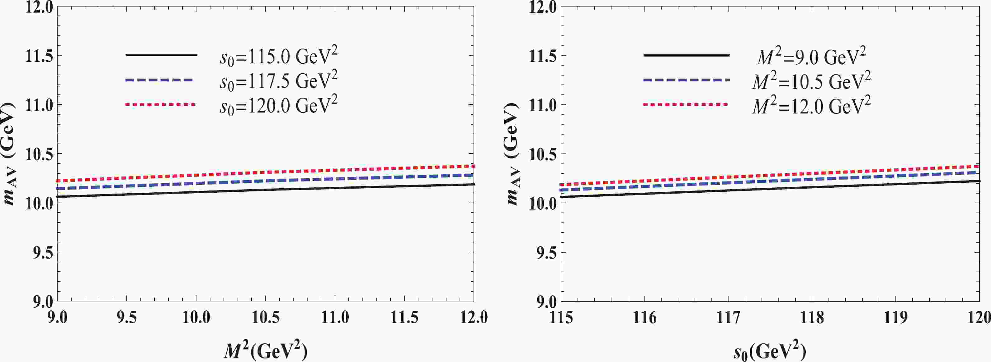
$ m_{\mathrm{AV}} $ and$ f_{\mathrm{AV}} $ , we have obtained$ \begin{aligned}[b] m_{\mathrm{AV}} =& (10215\pm 250)\; \mathrm{MeV}, \\ f_{\mathrm{AV}} =& (2.26\pm 0.57)\times 10^{-2}\; \mathrm{GeV}^{4}. \end{aligned} $

(20) In Eq. (20), the theoretical uncertainties of computations are shown as well. For the mass
$ m_{\mathrm{AV}} $ , these uncertainties are ±2.4% of the central value, and for the coupling$ f_{\mathrm{AV}} $ , they amount to ±25%, but in both cases, they remain within the limits accepted by the sum rule computations. In Fig. 1 , we plot our prediction for$ m_{\mathrm{AV}} $ as a function of$ M^{2} $ and$ s_{0} $ : one can see a mild dependence of$ m_{\mathrm{AV}} $ on these parameters. It is also evident that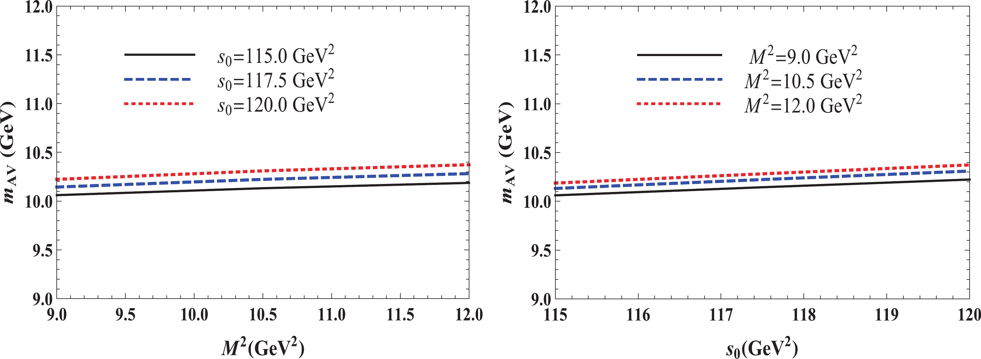
Figure 1. (color online) Dependence of the mass
$m_{\mathrm{AV}}$ on the Borel$M^{2}$ (left panel) and continuum threshold$s_{0}$ parameters (right panel).$ \begin{array}{l} \sqrt{s_{0}}-m_{\mathrm{AV}} = \left[ 510,740\right] \; \mathrm{MeV,} \end{array} $

(21) which is a reasonable mass gap between the ground-state and excited heavy tetraquarks.
Returning to the issue of the two-meson continuum, we can now compare the mass of the tetraquark
$ T_{b:\overline{s}}^{\mathrm{AV}} $ with the energy level of this continuum. It is clear that the two-meson continuum may be populated by pairs$ B^{-}B_{s}^{\ast } $ and$ B^{\ast -}\overline{B}_{s}^{0} $ , and that$ T_{b:\overline{s}}^{\mathrm{AV}} $ is$ \approx 480\; \mathrm{MeV} $ below it. This difference is comparable to (21); hence, one can ignore the two-meson continuum's impact on the physical parameters of$ T_{b:\overline{s}}^{\mathrm{AV}} $ .The mass
$ m_{{\cal{Z}}} $ and coupling$ f_{{\cal{Z}}} $ of the state$ {\cal{Z}}_{b:\overline{s}}^{0} $ are found from the sum rules by utilizing the following working windows for$ M^{2} $ and$ s_{0} $ $ \begin{array}{l} M^{2}\in \lbrack 5.5,6.5]\; \mathrm{GeV}^{2},\ s_{0}\in \lbrack 52,54]\; \mathrm{GeV}^{2}. \end{array} $

(22) The regions (22) satisfy standard restrictions associated with the sum rule computations. In fact, at
$ M^{2} = 5.5\; \mathrm{GeV}^{2} $ , the ratio R is$ 0.009 $ ; hence, the convergence of the sum rules is satisfied. The pole contribution$ \mathrm{PC} $ at$ M^{2} = 6.5\; \mathrm{GeV}^{2} $ and$ M^{2} = 5.5\; \mathrm{GeV}^{2} $ equals to$ 0.23 $ and$ 0.61 $ , respectively. At the minimum of$ M^{2} $ , the perturbative contribution constitutes 72% of the entire result and considerably exceeds that of nonperturbative terms.For
$ m_{{\cal{Z}}} $ and$ f_{{\cal{Z}}} $ , our computations yield$ \begin{split} m_{{\cal{Z}}} =& (6770\pm 150)\; \mathrm{MeV}, \\ f_{{\cal{Z}}} =& (6,3\pm 1.3)\times 10^{-3}\; \mathrm{GeV}^{4}. \end{split} $

(23) In Fig. 2, we depict the mass of the tetraquark
$ {\cal{Z}}_{b:\overline{s}}^{0} $ and demonstrate its dependence on$ M^{2} $ and$ s_{0} $ .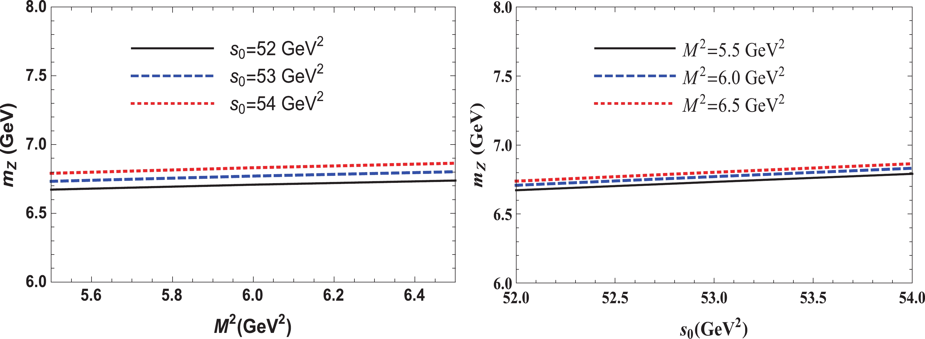
Figure 2. (color online) The mass
$m_{{\cal{Z}}}$ of the tetraquark${\cal{Z}}_{b:\overline{s}}^{0}$ as a function of the parameters$M^{2}$ (left panel) and$s_{0}$ (right panel).The mass of the axial-vector tetraquark
$ T_{b:\overline{s}}^{\mathrm{AV}} $ was calculated in Ref. [19] in the context of the QCD sum rule method, using different interpolating currents. Computations were performed with dimension$ 8 $ accuracy, and two lowest predictions for the mass of the axial-vector particle$ bb\overline{q}\overline{s} $ were obtained within ranges$ (10300\pm 300)\; \mathrm{MeV} $ and$ (10300\pm 400)\; \mathrm{MeV} $ . Our result is close to the central value of these predictions. The difference in theoretical errors can be attributed to the higher accuracy of our computations and more detailed quark propagators used in analysis. The authors of Ref. [19] noted the strong interaction stable nature of$ T_{b:\overline{s}}^{\mathrm{AV}} $ . As we will see below, our investigation proves that$ T_{b:\overline{s}}^{\mathrm{AV}} $ is stable against strong and radiative decays and can transform only through weak processes.The scalar tetraquark with the quark content
$ [bc][\overline{u}\overline{s}] $ was explored recently in Ref. [35]. The predicted mass of this state$ (7.14\pm 0.12)\; \mathrm{GeV} $ obtained there is larger than our prediction (23). Such a sizeable difference between the two results can be explained by some factors. Thus, in the present work, calculations have been performed by taking into account dimension$ \ 10 $ condensates, whereas in Ref. [35], the authors included nonperturbative terms up to the eighth dimension into analysis. We have used more detailed expressions for quark propagators, including the terms$ \sim g_{s}^{2}\langle \overline{q}q\rangle ^{2} $ and$ \sim \langle \overline{q}q\rangle \langle g_{s}^{2}G^{2}\rangle $ in the light and$ \sim \langle g_{s}^{3}G^{3}\rangle $ in the heavy quark propagators. However, in our view, the choice of the working windows for the parameters$ M^{2} $ and$ s_{0} $ is the main source of fixed discrepancies. The regions for$ M^{2} $ and$ s_{0} $ should be extracted from the analysis of constraints (17) and (18) imposed on the invariant amplitude$ \Pi (M^{2},s_{0}) $ . The$ \mathrm{PC} $ in the present investigation varies within 0.61-0.23, which corresponds to the boundaries of the Borel region. Let us emphasize that we extract the parameters$ m_{{\cal{Z}}} $ and$ f_{{\cal{Z}}} $ approximately in the middle region of the window (22), where the pole contribution is$ \mathrm{PC}\approx 0.42-0.45 $ . The working regions for$ M^{2} $ and$ s_{0} $ used in Ref. [35] ensure only$ \mathrm{PC}\approx 0.31 $ , which may generate differences in the extracted values of$ m_{{\cal{Z}}} $ . -
The analysis performed in the previous section confirms that the tetraquark
$ T_{b:\overline{s}}^{\mathrm{AV}} $ is stable against the strong and electromagnetic decays. Indeed, the mass of this state$ m_{\mathrm{AV}} = 10215\; \mathrm{MeV} $ is$ 480/477\; \mathrm{MeV} $ below the thresholds$ 10695/10692\; \mathrm{MeV} $ for its strong decays to mesons$ B^{-}B_{s}^{\ast } $ and$ B^{\ast -}\overline{B}_{s}^{0} $ , respectively. The maximum of the mass$ 10465\; \mathrm{MeV} $ is still below these limits. The threshold$ 10646\; \mathrm{MeV} $ for the process$ T_{b:\overline{s}}^{\mathrm{AV}}\rightarrow B^{-}\overline{B}_{s}^{0}\gamma $ also exceeds the maximal allowed value of$ m_{\mathrm{AV}} $ , which forbids this electromagnetic decay. Therefore, the full width and mean lifetime of$ T_{b:\overline{s}}^{\mathrm{AV}} $ are determined by its weak decays.There are different weak decay channels of
$ T_{b:\overline{s}}^{\mathrm{AV}} $ , which can be generated by sub-processes$ b\rightarrow W^{-}c $ and$ b\rightarrow W^{-}u $ . The decays triggered by the transition$ b\rightarrow W^{-}c $ are dominant processes relative to the ones connected with$ b\rightarrow W^{-}u $ : the latter decays are suppressed relative to the dominant decays by a factor$ |V_{bu}|^{2}/|V_{bc}|^{2} $ $ \simeq 0.01 $ , with$ V_{q_{1}q_{2}} $ being the Cabibbo-Khobayasi-Maskawa (CKM) matrix elements. In the present work, we restrict ourselves to the analysis of the dominant weak decays of$ T_{b:\overline{s}}^{\mathrm{AV}} $ (see Fig. 3).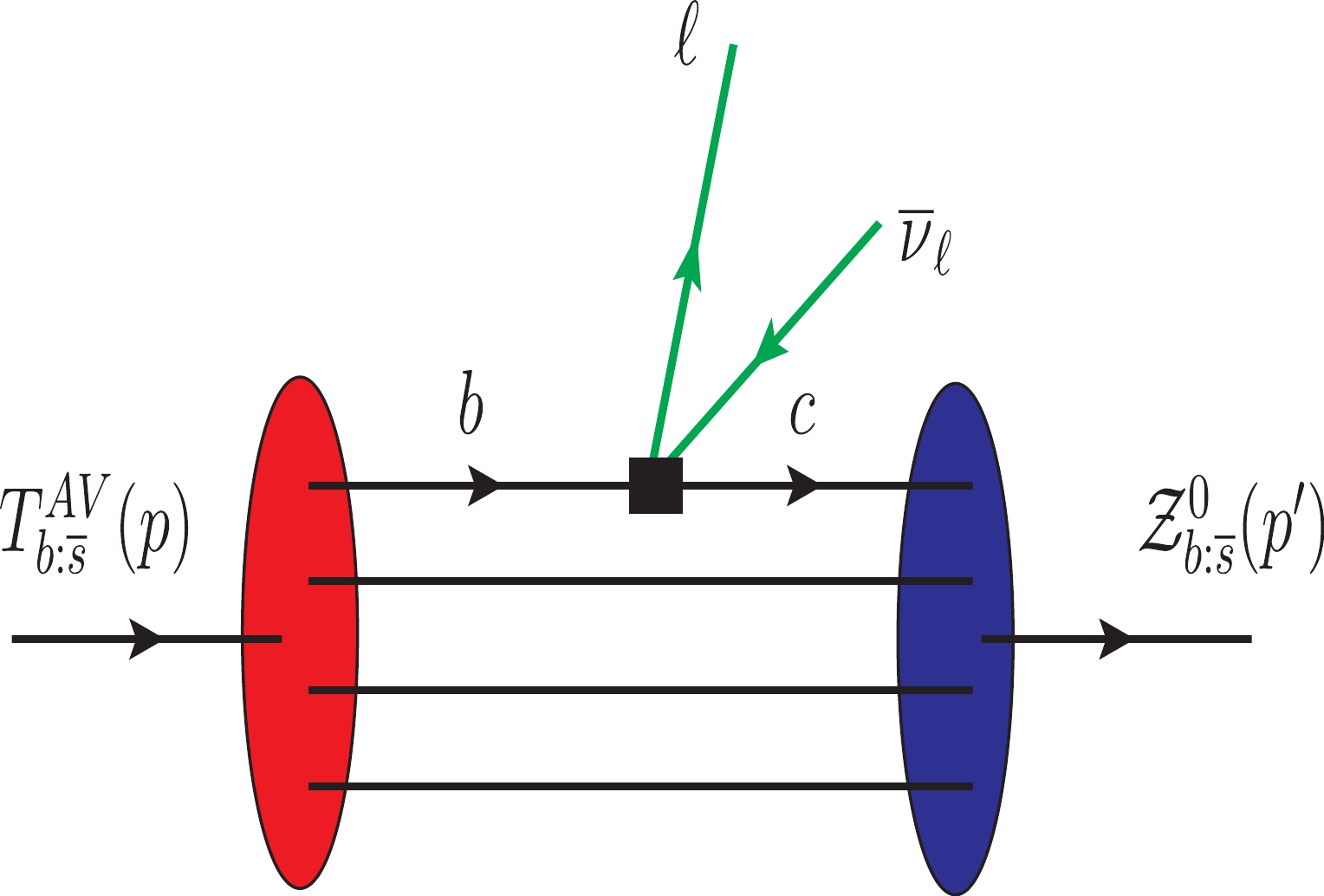
Figure 3. (color online) The Feynman diagram for the semileptonic decay
$T_{b:\overline{s}}^{\mathrm{AV}}\rightarrow {\cal{Z}}_{b:\overline{s}}^{0}l\overline{ \nu }_{l}$ . The black square denotes the effective weak vertex.The dominant processes themselves can be categorized into two groups: the first group contains the semileptonic decays
$ T_{b:\overline{s}}^{\mathrm{AV}}\rightarrow {\cal{Z}}_{b:\overline{s}}^{0}l\overline{\nu }_{l} $ , whereas the nonleptonic transitions$ T_{b:\overline{s}}^{\mathrm{AV}}\rightarrow {\cal{Z}}_{b:\overline{s}}^{0}M $ belong to the second group. In this section, we consider the semileptonic decays and calculate the partial widths of the processes$ T_{b:\overline{s}}^{\mathrm{AV}}\rightarrow {\cal{Z}}_{b:\overline{s}}^{0}l\overline{\nu }_{l} $ , where l is one of the lepton species$ e, \mu $ and$ \tau $ . Owing to the large mass difference between the initial and final tetraquarks,$ 3445\; \mathrm{MeV} $ , all of these semileptonic decays are kinematically allowed ones.The effective Hamiltonian to describe the subprocess
$ b\rightarrow W^{-}c $ at the tree-level is given by the expression$ \begin{array}{l} {\cal{H}}^{\mathrm{eff}} = \dfrac{G_{F}}{\sqrt{2}}V_{bc}\overline{c}\gamma _{\mu }(1-\gamma _{5})b\overline{l}\gamma ^{\mu }(1-\gamma _{5})\nu _{l}, \end{array} $

(24) with
$ G_{F} $ and$ V_{bc} $ being the Fermi coupling constant and CKM matrix element, respectively. A matrix element of$ {\cal{H}}^{\mathrm{eff}} $ between the initial and final tetraquarks is equal to$ \begin{array}{l} \langle {\cal{Z}}_{b:\overline{s}}^{0}(p^{\prime })|{\cal{H}}^{\mathrm{eff}}|T_{b:\overline{s}}^{\mathrm{AV}}(p)\rangle = L_{\mu }H^{\mu }, \end{array} $

(25) where
$ L_{\mu } $ and$ H^{\mu } $ are the leptonic and hadronic factors, respectively. A treatment of$ L_{\mu } $ is trivial; therefore, we consider the matrix element$ H^{\mu } $ in a detailed form, which depends on the parameters of the tetraquarks. After factoring out the constant factors,$ H^{\mu } $ is the matrix element of the current$ \begin{array}{l} J_{\mu }^{\mathrm{tr}} = \overline{c}\gamma _{\mu }(1-\gamma _{5})b. \end{array} $

(26) The matrix element
$ \langle {\cal{Z}}_{b:\overline{s}}^{0}(p^{\prime })|J_{\mu }^{\mathrm{tr}}|T_{b:\overline{s}}^{\mathrm{AV}}(p)\rangle $ describes the weak transition of the axial-vector tetraquark to the scalar particle and is expressible in terms of four weak form factors$ G_{i}(q^{2}) $ that parametrize long-distance dynamical effects of this transformation [36,37]$ \begin{split} \langle {\cal{Z}}_{b:\overline{s}}^{0}(p^{\prime })|J_{\mu }^{\mathrm{tr} }|T_{b:\overline{s}}^{\mathrm{AV}}(p)\rangle =& \widetilde{G} _{0}(q^{2})\epsilon _{\mu }+\widetilde{G}_{1}(q^{2})(\epsilon p^{\prime })P_{\mu } \\& +\widetilde{G}_{2}(q^{2})(\epsilon p^{\prime })q_{\mu }\\&+ {\rm i}\widetilde{G} _{3}(q^{2})\varepsilon _{\mu \nu \alpha \beta }\epsilon ^{\nu }p^{\alpha }p^{\prime }{}^{\beta }. \end{split} $

(27) The scaled functions
$ \widetilde{G}_{i}(q^{2}) $ are connected with the dimensionless form factors$ G_{i}(q^{2}) $ by the equalities$ \begin{array}{l} \widetilde{G}_{0}(q^{2}) = \widetilde{m}G_{0}(q^{2}),\ \widetilde{G}_{j}(q^{2}) = \dfrac{G_{j}(q^{2})}{\widetilde{m}},\ j = 1,2,3. \end{array} $

(28) Here,
$ \widetilde{m} = m_{\mathrm{AV}}+m_{{\cal{Z}}} $ ,$ p_{\mu } $ and$ \epsilon _{\mu } $ are the momentum and polarization vector of the tetraquark$ T_{b:\overline{s}}^{\mathrm{AV}} $ ,$ p^{\prime } $ is the momentum of the scalar state$ {\cal{Z}}_{b:\overline{s}}^{0} $ . We use also$ P_{\mu } = p_{\mu }^{\prime }+p_{\mu } $ and$ q_{\mu } = p_{\mu }-p_{\mu }^{\prime } $ , the latter being the momentum transferred to the leptons. It is evident that$ q^{2} $ varies within$ m_{l}^{2}\leqslant q^{2}\leqslant (m_{\mathrm{AV}}-m_{{\cal{Z}}})^{2}, $ where$ m_{l} $ is the mass of a lepton l.The sum rules for the form factors
$ G_{i}(q^{2}) $ can be obtainedby analyzing the three-point correlation function$ \begin{split} \Pi _{\mu \nu }(p,p^{\prime }) =& i^{2}\displaystyle\int {\rm d}^{4}x{\rm d}^{4}y{\rm e}^{{\rm i}(p^{\prime }y-px)} \\& \times \langle 0|{\cal{T}}\{J_{{\cal{Z}}}(y)J_{\nu }^{\mathrm{tr}}(0)J_{\mu }^{^{\dagger }}(x)\}|0\rangle . \end{split} $

(29) To this end, we have to express
$ \Pi _{\mu \nu }(p,p^{\prime }) $ using the masses and couplings of the tetraquarks and thus determine the physical side of the sum rules$ \Pi _{\mu \nu }^{\mathrm{Phys}}(p,p^{\prime }) $ . The function$ \Pi _{\mu \nu }^{\mathrm{Phys}}(p,p^{\prime }) $ can be presented as$ \begin{split} \Pi _{\mu \nu }^{\mathrm{Phys}}(p,p^{\prime }) =& \dfrac{\langle 0|J_{\mathcal{ Z}}|{\cal{Z}}_{b:\overline{s}}^{0}(p^{\prime })\rangle \langle {\cal{Z}} _{b:\overline{s}}^{0}(p^{\prime })|J_{\nu }^{\mathrm{tr}}|T_{b:\overline{s} }^{\mathrm{AV}}(p,\epsilon )\rangle }{(p^{2}-m_{\mathrm{AV}}^{2})(p^{\prime 2}-m_{{\cal{Z}}}^{2})} \\& \times \langle T_{b:\overline{s}}^{\mathrm{AV}}(p,\epsilon )|J_{\mu }^{^{\dagger }}|0\rangle +\cdots, \end{split} $

(30) where we take into account the contribution of the ground-state particles and denote the effects of the excited and continuum states by dots.
The phenomenological side of the sum rules can be simplified by substituting into Eq. (30) the expressions of matrix elements in terms of the tetraquarks' masses and couplings as well as weak transition form factors. For these purposes, we employ Eqs. (7) and (27) and define the matrix element of
$ {\cal{Z}}_{b:\overline{s}}^{0} $ $ \begin{array}{l} \langle 0|J_{{\cal{Z}}}|{\cal{Z}}_{b:\overline{s}}^{0}(p^{\prime })\rangle = f_{{\cal{Z}}}m_{{\cal{Z}}}. \end{array} $

(31) Then, one gets
$ \begin{split} \Pi _{\mu \nu }^{\mathrm{Phys}}(p,p^{\prime }) =& \dfrac{f_{\mathrm{AV}}m_{ \mathrm{AV}}f_{{\cal{Z}}}m_{{\cal{Z}}}}{(p^{2}-m_{\mathrm{AV} }^{2})(p^{\prime 2}-m_{{\cal{Z}}}^{2})} \\& \times \left\{ \widetilde{G}_{0}(q^{2})\left( -g_{\mu \nu }+\dfrac{p_{\mu }p_{\nu }}{m_{\mathrm{AV}}^{2}}\right) +\left[ \widetilde{G} _{1}(q^{2})P_{\mu }\right. \right. \\& \left. +\widetilde{G}_{2}(q^{2})q_{\mu }\right] \left( -p_{\nu }^{\prime }+ \dfrac{m_{\mathrm{AV}}^{2}+m_{{\cal{Z}}}^{2}-q^{2}}{2m_{\mathrm{AV}}^{2}} p_{\nu }\right) \\& -{\rm i}\widetilde{G}_{3}(q^{2})\varepsilon _{\mu \nu \alpha \beta }p^{\alpha }p^{\prime }{}^{\beta }\Bigg\} +\cdots. \end{split} $

(32) We should also calculate the correlation function in terms of the quark propagators and find
$ \Pi _{\mu \nu }^{\mathrm{OPE}}(p,p^{\prime }) $ . The function$ \Pi _{\mu \nu }^{\mathrm{OPE}}(p,p^{\prime }) $ is the second side of the sum rules and has the following form$ \begin{aligned}[b] \Pi _{\mu \nu }^{\mathrm{OPE}}(p,p^{\prime }) =& \displaystyle\int {\rm d}^{4}x{\rm d}^{4}y{\rm e}^{{\rm i}(p^{\prime }y-px)}\left\{ \mathrm{Tr}\left[ \gamma _{5} \widetilde{S}_{s}^{ba^{\prime }}(x-y)\right. \right. \left. \times \gamma _{5}S_{u}^{a^{\prime }b}(x-y)\right] \left( \mathrm{Tr }\left[ \gamma _{\mu }\widetilde{S}_{b}^{aa^{\prime }}(y-x)\gamma _{5}S_{c}^{bi}(y)\gamma _{\nu }(1-\gamma _{5})\right. \right. \left. \times S_{b}^{ib^{\prime }}(-x)\right] \\& +\mathrm{Tr}\left[ \gamma _{\mu }\widetilde{S}_{b}^{ia^{\prime }}(-x)(1-\gamma _{5})\gamma _{\nu } \widetilde{S}_{c}^{bi}(y)\gamma _{5}\right. \left. \left. \times S_{b}^{ab^{\prime }}(y-x)\right] \right) -\mathrm{Tr} \left[ \gamma _{5}\widetilde{S}_{s}^{b^{\prime }a}(x-y)\gamma _{5}S_{u}^{a^{\prime }b}(x-y)\right] \\& \times \left( \mathrm{Tr}\left[ \gamma _{\mu }\widetilde{S} _{b}^{aa^{\prime }}(y-x)\gamma _{5}S_{c}^{bi}(y)\gamma _{\nu }(1-\gamma _{5})S_{b}^{ib^{\prime }}(-x)\right] \right. \left. \left. +\mathrm{Tr}\left[ \gamma _{\mu }\widetilde{S} _{b}^{ia^{\prime }}(-x)(1-\gamma _{5})\gamma _{\nu }\widetilde{S} _{c}^{bi}(y)\gamma _{5}S_{b}^{ab^{\prime }}(y-x)\right] \right) \right\}. \\ \end{aligned} $

(33) To extract expressions of the form factors
$ G_{i}(q^{2}) $ , we equate invariant amplitudes corresponding to the same Lorentz structures both in$ \Pi _{\mu \nu }^{\mathrm{Phys}}(p,p^{\prime }) $ and$ \Pi _{\mu \nu }^{\mathrm{OPE}}(p,p^{\prime }) $ , carry out double Borel transformations over the variables$ p^{\prime 2} $ and$ p^{2} $ , and perform continuum subtraction. For instance, to extract the sum rule for$ \widetilde{G}_{0}(q^{2}) $ , we use the structure$ g_{\mu \nu } $ , whereas for$ \widetilde{G}_{3}(q^{2}) $ , the term$ \sim \varepsilon _{\mu \nu \alpha \beta }p^{\alpha }p^{\prime }{}^{\beta } $ can be employed. The sum rules for the scaled form factors$ \widetilde{G}_{i}(q^{2}) $ can be written in a single formula$ \begin{split} \widetilde{G}_{i}(\bf{M}^{2},\bf{s}_{0},q^{2}) =& \dfrac{1}{f_{\mathrm{ AV}}m_{\mathrm{AV}}f_{{\cal{Z}}}m_{{\cal{Z}}}}\displaystyle\int_{{\cal{M}} ^{2}}^{s_{0}}{\rm d}s{\rm e}^{(m_{\mathrm{AV}}^{2}-s)/M_{1}^{2}} \\& \times \displaystyle\int_{\widetilde{{\cal{M}}}^{2}}^{s_{0}^{\prime }}{\rm d}s^{\prime }\rho _{i}(s,s^{\prime }){\rm e}^{(m_{{\cal{Z}}}^{2}-s^{\prime })/M_{2}^{2}}, \end{split} $

(34) where
$ \rho _{i}(s,s^{\prime }) $ are spectral densities computed as the imaginary parts of the corresponding terms in$ \Pi _{\mu \nu }^{\mathrm{OPE}}(p,p^{\prime }) $ . They contain perturbative and nonperturbative contributions and are found in the present work with dimension-6 accuracy. In Eq. (34),${\bf M}^{2} = (M_{1}^{2},M_{2}^{2})$ and${\bf s}_{0} = (s_{0},\ s_{0}^{\prime })$ are the Borel and continuum threshold parameters, respectively. The pair of parameters ($ M_{1}^{2} $ ,$ s_{0} $ ) corresponds to the initial tetraquark's channels, whereas ($ M_{2}^{2} $ ,$ s_{0}^{\prime } $ ) describes the final-state tetraquark.As usual, the form factors
$ \widetilde{G}_{i}(\bf{M}^{2},\bf{s}_{0},q^{2}) $ contain various input parameters, which should be determined before numerical analysis. The vacuum condensates of quark, gluon, and mixed operators are already presented in Eq. (15). The masses and couplings of the tetraquarks$ T_{b:\overline{s}}^{\mathrm{AV}} $ and$ {\cal{Z}}_{b:\overline{s}}^{0} $ have been extracted in Section II. The Borel and continuum threshold parameters$ \bf{M}^{2} $ and$ \bf{s}_{0} $ should be chosen so as to meet all restrictions of sum rule computations. One has also to bear in mind that$ \widetilde{G}_{i}(\bf{M}^{2},\bf{s}_{0},q^{2}) $ depends on the masses and couplings of the initial and final tetraquarks, which have been evaluated also in the context of the sum rule approach. We fix the auxiliary parameters ($ M_{1}^{2} $ ,$ s_{0} $ ) and ($ M_{2}^{2} $ ,$ s_{0}^{\prime } $ ) as in the corresponding mass computations, because they satisfy standard constraints of three-point sum rule calculations and do not generate additional uncertainties in the spectroscopic parameters of relevant tetraquarks.The form factors
$ \widetilde{G}_{i}(q^{2}) $ determine the differential decay rate${\rm d}\Gamma /{\rm d}q^{2}$ of the semileptonic decay$ T_{b:\overline{s}}^{\mathrm{AV}}\rightarrow {\cal{Z}}_{b:\overline{s}}^{0}l\overline{\nu }_{l} $ , the explicit expression of which can be found in Ref. [3]. The partial width of the process is equal to an integral of this rate over the momentum transfer$ q^{2} $ within the limits$ m_{l}^{2}\leqslant q^{2}\leqslant (m_{\mathrm{AV}}-m_{{\cal{Z}}})^{2} $ . Our results for the form factors are plotted in Fig. 4. The QCD sum rules lead to reliable predictions at$ m_{l}^{2}\leqslant q^{2}\leqslant 8\; \mathrm{GeV}^{2} $ . However, these predictions do not cover the entire integration region$ m_{l}^{2}\leqslant q^{2}\leqslant 11.87\; \mathrm{GeV}^{2} $ . To solve this problem, one has to introduce extrapolation functions$ {\cal{G}}_{i}(q^{2}) $ of a relatively simple analytic form, which, at$ q^{2} $ accessible to the QCD sum rules, coincide with their predictions but can be used in the entire region.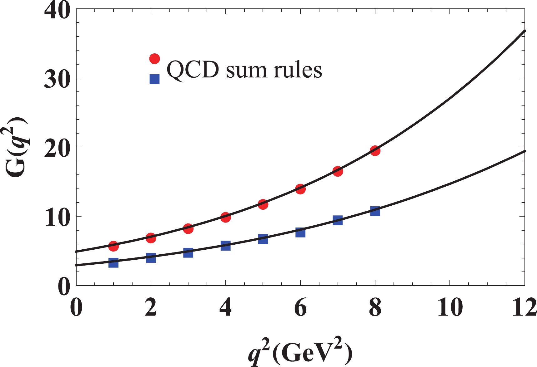
Figure 4. (color online) Sum rule results for the form factors
$ G_{0}(q^{2}) $ (red circles) and$ G_{1}(q^{2}) $ (blue squares). The solid curves are fit functions$ {\cal{G}}_{0}(q^{2}) $ and$ {\cal{G}}_{1}(q^{2}) $ .For these purposes, we choose to work with the functions
$ \begin{array}{l} {\cal{G}}_{i}(q^{2}) = {\cal{G}}_{0}^{i}\exp \left[ g_{1}^{i}\dfrac{q^{2}}{ m_{\mathrm{AV}}^{2}}+g_{2}^{i}\left( \dfrac{q^{2}}{m_{\mathrm{AV}}^{2}} \right) ^{2}\right], \end{array} $

(35) in which the parameters
$ {\cal{G}}_{0}^{i},\; g_{1}^{i} $ , and$ g_{2}^{i} $ should be fitted to satisfy the sum rules' predictions. The parameters of the functions$ {\cal{G}}_{i}(q^{2}) $ , obtained numerically, are presented in Table 1. The functions$ {\cal{G}}_{i}(q^{2}) $ are also shown in Fig. 4 : one can see a good agreement between the sum rule predictions and fit functions.${\cal{G}}_{i}(q^{2})$ 

${\cal{G}}_{0}^{i}$ 

$g_{1}^{i}$ 

$g_{2}^{i}$ 

${\cal{G}}_{0}(q^{2})$ 

$4.91$ 

$19.29$ 

$-15.34$ 

${\cal{G}}_{1}(q^{2})$ 

$2.94$ 

$18.73$ 

$-20.09$ 

${\cal{G}}_{2}(q^{2})$ 

$-22.67$ 

$20.50$ 

$-22.95$ 

${\cal{G}}_{3}(q^{2})$ 

$-21.14$ 

$20.77$ 

$-23.62$ 

Table 1. Parameters of the extrapolating functions
${\cal{G}}_{i}(q^{2})$ .In the numerical computations for the Fermi constant, CKM matrix elements, and masses of leptons, we use
$ \begin{aligned}[b] G_{F} &= 1.16637\times 10^{-5}\; \mathrm{GeV}^{-2}, \\ |V_{bc}| &= (42.2\pm 0.08)\times 10^{-3}, \end{aligned} $

(36) $ m_{e} = 0.511\; \mathrm{MeV} $ ,$ m_{\mu } = 105.658\; \mathrm{MeV} $ , and$m_{\tau } = $ $ (1776.82 \pm 0.16)\; \mathrm{MeV} $ [38]. The predictions obtained for the partial widths of the semileptonic decays$ T_{b:\overline{s}}^{\mathrm{AV}}\rightarrow {\cal{Z}}_{b:\overline{s}}^{0}l\overline{\nu }_{l} $ are written as$ \begin{aligned}[b] \Gamma (T_{b:\overline{s}}^{\mathrm{AV}} \rightarrow {\cal{Z}}_{b: \overline{s}}^{0}e^{-}\overline{\nu }_{e}) &= (5.34\pm 1.43)\times 10^{-8}\; \mathrm{MeV}, \\ \Gamma (T_{b:\overline{s}}^{\mathrm{AV}} \rightarrow {\cal{Z}}_{b: \overline{s}}^{0}\mu ^{-}\overline{\nu }_{\mu }) &= (5.32\pm 1.41)\times 10^{-8}\; \mathrm{MeV}, \\ \Gamma (T_{b:\overline{s}}^{\mathrm{AV}} \rightarrow {\cal{Z}}_{b: \overline{s}}^{0}\tau ^{-}\overline{\nu }_{\tau }) &= (2.15\pm 0.54)\times 10^{-8}\; \mathrm{MeV}, \\ \end{aligned} $

(37) and are main results of this section.
-
The second class of the weak decays of the tetraquark
$ T_{b:\overline{s}}^{\mathrm{AV}} $ are the processes$ T_{b:\overline{s}}^{\mathrm{AV}}\rightarrow {\cal{Z}}_{b:\overline{s}}^{0}M $ , which may affect the full width and lifetime of the tetraquark$ T_{b:\overline{s}}^{\mathrm{AV}} $ . Here, we study the nonleptonic weak decays$ T_{b:\overline{s}}^{\mathrm{AV}}\rightarrow {\cal{Z}}_{b:\overline{s}}^{0}M $ of the tetraquark$ T_{b:\overline{s}}^{\mathrm{AV}} $ in the framework of the QCD factorization method. This approach was applied for investigating the nonleptonic decays of conventional mesons [39,40] but can be also used for investigating the decays of tetraquarks. Thus, the nonleptonic decays of scalar exotic mesons$ T_{b:\overline{s}}^{-} $ ,$ T_{b:\overline{s}}^{-} $ ,$ Z_{bc}^{0} $ , and$ T_{bs;\overline{u}\overline{d}}^{-} $ were explored using this approach in Refs. [25,26,41,42], respectively. The weak decays of double- and fully-heavy tetraquarks were analyzed in Refs. [43,44].We consider processes where M is one of the vector mesons
$ \rho ^{-} $ ,$ K^{\ast }(892) $ ,$ \ D^{\ast }(2010)^{-} $ , and$ \ D_{s}^{\ast -} $ . We provide details of analysis for the decay$ T_{b:\overline{s}}^{\mathrm{AV}}\rightarrow {\cal{Z}}_{b:\overline{s}}^{0}\rho ^{-} $ and write the final predictions for other channels. The relevant Feynman diagram is shown in Fig. 5.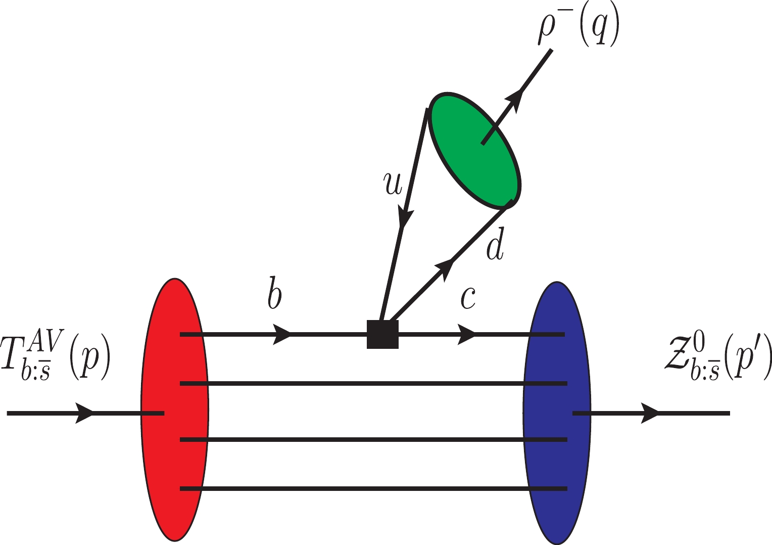
Figure 5. (color online) The diagram for the nonleptonic decay
$T_{b:\overline{s}}^{\mathrm{AV}}\rightarrow {\cal{Z}}_{b:\overline{s}}^{0}\rho ^{-}$ .At the quark level, the effective Hamiltonian for this decay is given by the expression
$ \begin{array}{l} {\cal{H}}_{\mathrm{n.-lep}}^{\mathrm{eff}} = \dfrac{G_{F}}{\sqrt{2}} V_{bc}V_{ud}^{\ast }\left[ c_{1}(\mu )Q_{1}+c_{2}(\mu )Q_{2}\right] , \end{array} $

(38) where
$ \begin{split} Q_{1} &= \left( \overline{d}_{i}u_{i}\right) _{\mathrm{V-A}}\left( \overline{c}_{j}b_{j}\right) _{\mathrm{V-A}}, \\ Q_{2} &= \left( \overline{d}_{i}u_{j}\right) _{\mathrm{V-A}}\left( \overline{c}_{j}b_{i}\right) _{\mathrm{V-A}}, \end{split} $

(39) i and j are the color indices, and
$ \left( \overline{q}_{1}q_{2}\right) _{\mathrm{V-A}} $ means$ \begin{array}{l} \left( \overline{q}_{1}q_{2}\right) _{\mathrm{V-A}} = \overline{q}_{1}\gamma _{\mu }(1-\gamma _{5})q_{2}. \end{array} $

(40) The short-distance Wilson coefficients
$ c_{1}(\mu ) $ and$ c_{2}(\mu ) $ are given on the factorization scale$ \mu $ .In the factorization method, the amplitude of the decay
$ T_{b:\overline{s}}^{\mathrm{AV}}\rightarrow {\cal{Z}}_{b:\overline{s}}^{0}\rho ^{-} $ has the form$ \begin{split} {\cal{A}} =& \dfrac{G_{F}}{\sqrt{2}}V_{bc}V_{ud}^{\ast }a(\mu )\langle \rho ^{-}(q)|\left( \overline{d}_{i}u_{i}\right) _{\mathrm{V-A}}|0\rangle \\& \times \langle {\cal{Z}}_{b:\overline{s}}^{0}(p^{\prime })|\left( \overline{c}_{j}b_{j}\right) _{\mathrm{V-A}}|T_{b:\overline{s}}^{\mathrm{AV} }(p)\rangle , \end{split} $

(41) where
$ \begin{array}{l} a(\mu ) = c_{1}(\mu )+\dfrac{1}{N_{c}}c_{2}(\mu ), \end{array} $

(42) with
$ N_{c} = 3 $ being the number of quark colors. The only unknown matrix element$ \langle \rho ^{-}(q)|\left( \overline{d}_{i}u_{i}\right) _{\mathrm{V-A}}|0\rangle $ in$ {\cal{A}} $ can be defined in the following form$ \begin{array}{l} \langle \rho ^{-}(q)|\left( \overline{d}_{i}u_{i}\right) _{\mathrm{V-A} }|0\rangle = f_{\rho }m_{\rho }\epsilon _{\mu }^{\ast }(q). \end{array} $

(43) Then, it is evident that
$ \begin{split} {\cal{A}} =& i\dfrac{G_{F}}{\sqrt{2}}f_{\rho }V_{bc}V_{ud}^{\ast }a(\mu ) \left[ \widetilde{G}_{0}(q^{2})\epsilon _{\mu }(p)\epsilon ^{\ast \mu }(q)\right. \\& +2\widetilde{G}_{1}(q^{2})(p^{\prime }\epsilon (p))(p^{\prime }\epsilon ^{\ast }(q)) \\& \left. +i\widetilde{G}_{3}(q^{2})\varepsilon _{\mu \nu \alpha \beta }\epsilon ^{\ast \mu }(q)\epsilon ^{\nu }(p)p^{\alpha }p^{\prime }{}^{\beta } \right] . \end{split} $

(44) The decay modes
$ T_{b:\overline{s}}^{\mathrm{AV}}\rightarrow {\cal{Z}}_{b:\overline{s}}^{0}K^{\ast }(892)[D^{\ast }(2010)^{-} $ ,$ D_{s}^{\ast -}] $ can be analyzed in a similar way. To this end, we have to replace in relevant expressions the spectroscopic parameters ($ m_{\rho },f_{\rho } $ ) of the$ \rho $ meson with masses and decay constants of the mesons$ K^{\ast }(892) $ ,$ D^{\ast }(2010)^{-} $ , and$ D_{s}^{\ast -} $ and make the substitutions$ V_{ud}\rightarrow V_{us} $ ,$ V_{cd} $ , and$ V_{cs} $ .The width of the nonleptonic decay
$ T_{b:\overline{s}}^{\mathrm{AV}}\rightarrow {\cal{Z}}_{b:\overline{s}}^{0}\rho ^{-} $ can be evaluated using the expression$ \begin{array}{l} \Gamma = \dfrac{|{\cal{A}}|^{2}}{24\pi m_{\mathrm{AV}}^{2}}\lambda \left( m_{\mathrm{AV}},m_{{\cal{Z}}},m_{\rho }\right) , \end{array} $

(45) where
$ \begin{split} \lambda (a,b,c) =& \dfrac{1}{2a}\left[ a^{4}+b^{4}+c^{4}\right. \\& \left. -2\left( a^{2}b^{2}+a^{2}c^{2}+b^{2}c^{2}\right) \right] ^{1/2}. \end{split} $

(46) The key component in Eq. (45), i.e.,
$ |{\cal{A}}|^{2} $ has a simple form$ \begin{array}{l} |{\cal{A}}|^{2} = \displaystyle\sum\limits_{j = 0,1,2}H_{j}\widetilde{G}_{j}^{2}+H_{3}\widetilde{G}_{0}\widetilde{G}_{1}, \end{array} $

(47) where
$ H_{j} $ are given by the expressions$ \begin{split} H_{0} =& \dfrac{m_{\rho }^{4}+(m_{\mathrm{AV}}^{2}-m_{{\cal{Z}} }^{2})^{2}+2m_{\rho }^{2}\left( 5m_{\mathrm{AV}}^{2}-m_{{\cal{Z}} }^{2}\right) }{4m_{\rho }^{2}m_{\mathrm{AV}}^{2}}, \\ H_{1} =& \dfrac{\left[ m_{\rho }^{4}+(m_{\mathrm{AV}}^{2}-m_{{\cal{Z}} }^{2})^{2}-2m_{\rho }^{2}\left( m_{\mathrm{AV}}^{2}+m_{{\cal{Z}} }^{2}\right) \right] ^{2}}{4m_{\rho }^{2}m_{\mathrm{AV}}^{2}}, \\ H_{2} =& \frac{1}{2}\left[ m_{\rho }^{4}+(m_{\mathrm{AV}}^{2}-m_{{\cal{Z}} }^{2})^{2}-2m_{\rho }^{2}\left( m_{\mathrm{AV}}^{2}+m_{{\cal{Z}} }^{2}\right) \right] , \\ H_{3} =& -\dfrac{1}{2m_{\rho }^{2}m_{\mathrm{AV}}^{2}}\left[ m_{\rho }^{6}+(m_{ \mathrm{AV}}^{2}-m_{{\cal{Z}}}^{2})^{3}-m_{\rho }^{4}\left( m_{\mathrm{AV} }^{2}+3m_{{\cal{Z}}}^{2}\right)\right. \\& \left. -m_{\rho }^{2}\left( m_{\mathrm{ AV}}^{4}+2m_{{\cal{Z}}}^{2}m_{\mathrm{AV}}^{2}-3m_{{\cal{Z}}}^{2}\right) \right] . \end{split} $

(48) In Eq. (47), we take into account that the weak form factors
$ \widetilde{G}_{j} $ are real functions of$ q^{2} $ , and their values for the process$ T_{b:\overline{s}}^{\mathrm{AV}}\rightarrow {\cal{Z}}_{b:\overline{s}}^{0}M $ are fixed at$ q^{2} = m_{M}^{2} $ .All input information necessary for numerical analysis is presented in Table 2: the table lists the spectroscopic parameters of the final-state mesons and the CKM matrix elements. For the masses of the vector mesons, we use information from PDG [38]. The decay constants of mesons
$ \rho $ and$ K^{\ast }(892) $ are also taken from this source. The decay constants of mesons$ D^{\ast } $ and$ D_{s}^{\ast } $ are theoretical predictions obtained in the lattice QCD framework [45]. The coefficients$ c_{1}(m_{b}) $ , and$ c_{2}(m_{b}) $ with next-to-leading order QCD corrections have been borrowed from Refs. [46-48]Quantity Value $ m_{\rho} $ 

$ (775.26 \pm 0.25)\; \mathrm{MeV} $ 

$ m_{K^{\star}} $ 

$ (891.66\pm 0.26)\; \mathrm{MeV} $ 

$ m_{D^{\star}} $ 

$ (2010.26 \pm 0.05)\; \mathrm{MeV} $ 

$ m_{D_s^{\star}} $ 

$ (2112.2 \pm 0.4)\; \mathrm{MeV} $ 

$ f_{\rho } $ 

$ (210 \pm 4)\; \mathrm{MeV} $ 

$ f_{K^{\star}} $ 

$ (204 \pm 7)\; \mathrm{MeV} $ 

$ f_{D^{\star}} $ 

$ (223.5 \pm 8.4)\; \mathrm{MeV} $ 

$ f_{D_s^{\star}} $ 

$ (268.8 \pm 6.6)\; \mathrm{MeV} $ 

$ |V_{ud}| $ 

$ 0.97420\pm 0.00021 $ 

$ |V_{us}| $ 

$ 0.2243\pm 0.0005 $ 

$ |V_{cd}| $ 

$ 0.218\pm 0.004 $ 

$ |V_{cs}| $ 

$ 0.997\pm 0.017 $ 

Table 2. Masses and decay constants of the final-state vector mesons and CKM matrix elements.
$ \begin{array}{l} c_{1}(m_{b}) = 1.117,\ c_{2}(m_{b}) = -0.257. \end{array} $

(49) For the decay
$ T_{b:\overline{s}}^{\mathrm{AV}}\rightarrow {\cal{Z}}_{b:\overline{s}}^{0}\rho ^{-} $ , our calculations yield$ \begin{array}{l} \Gamma (T_{b:\overline{s}}^{\mathrm{AV}} \rightarrow {\cal{Z}}_{b: \overline{s}}^{0}\rho ^{-}) = \left( 3.47\pm 0.92\right) \times 10^{-10}\; \mathrm{MeV}. \\ \end{array} $

(50) The partial widths of the remaining three nonleptonic decays are presented below
$ \begin{split} \Gamma (T_{b:\overline{s}}^{\mathrm{AV}}\rightarrow {\cal{Z}}_{b: \overline{s}}^{0}K^{\ast }(892)) =& \left( 1.47\pm 0.37\right) \times 10^{-11}\; \mathrm{MeV}, \\ \Gamma (T_{b:\overline{s}}^{\mathrm{AV}}\rightarrow {\cal{Z}}_{b: \overline{s}}^{0}D^{\ast }(2010)^{-}) =& \left( 1.54\pm 0.39\right) \times 10^{-11}\; \mathrm{MeV}, \\ \Gamma (T_{b:\overline{s}}^{\mathrm{AV}}\rightarrow {\cal{Z}}_{b: \overline{s}}^{0}D_{s}^{\ast }{}^{-}) =& \left( 4.97\pm 1.32\right) \times 10^{-10}\; \mathrm{MeV}. \\ \end{split} $

(51) It is evident that the parameters of the processes
$T_{b:\overline{s}}^{\mathrm{AV}}\rightarrow $ $ {\cal{Z}}_{b:\overline{s}}^{0}\rho ^{-} $ and$ T_{b:\overline{s}}^{\mathrm{AV}}\rightarrow {\cal{Z}}_{b:\overline{s}}^{0}D_{s}^{\ast }{}^{-} $ are comparable to each other and may affect predictions for the tetraquark$ T_{b:\overline{s}}^{\mathrm{AV}} $ : the other two decays can be safely neglected in the computation of$ \Gamma _{\mathrm{full}} $ and$ \tau $ . Then, using Eqs. (37), (50), and (51), we find$ \begin{split} \Gamma _{\mathrm{full}} &= (12.9\pm 2.1)\times 10^{-8}\; \mathrm{MeV}, \\ \tau &= 5.1_{-0.71}^{+0.99}\times 10^{-15}\; \mathrm{s}, \end{split} $

(52) which are principally new predictions of the present article.
-
We have calculated the mass, width, and lifetime of the stable axial-vector tetraquark
$ T_{b:\overline{s}}^{\mathrm{AV}} $ with the content$ bb\overline{u}\overline{s} $ . This particle is a strange partner of the tetraquark$ T_{bb}^{-} $ , which was explored in Ref. [3]. The width and lifetime of$ T_{bb}^{-} $ $ \begin{split} \widetilde{\Gamma }_{\mathrm{full}} &= (7.17\pm 1.23)\times 10^{-8}\; \mathrm{ MeV}, \\ \widetilde{\tau } & = 9.18_{-1.34}^{+1.90}\times 10^{-15}\; \mathrm{s}, \end{split} $

(53) are comparable to those of the tetraquark
$ T_{b:\overline{s}}^{\mathrm{AV}} $ .The tetraquark
$ T_{b:\overline{s}}^{\mathrm{AV}} $ is the last of the four scalar and axial-vector states$ bb\overline{u}\overline{s} $ and$ bb\overline{u}\overline{d} $ considered in our works. The spectroscopic parameters and widths of the scalar tetraquarks$ T_{b:\overline{s}}^{-} $ and$ T_{b:\overline{d}}^{-} $ were calculated in Refs. [25,26]. We demonstrated there that$ T_{b:\overline{s}}^{-} $ and$ T_{b:\overline{d}}^{-} $ are stable against the strong and electromagnetic decays, and using the dominant semileptonic and nonleptonic decay channels of these particles, we estimated their full widths and lifetimes. The information about the tetraquarks composed of a heavy diquark$ bb $ and light antidiquarks is presented in Table 3.Tetraquark $(J^{P})$ 

Mass/ $\mathrm{MeV}$ 

Width/ $\mathrm{MeV}$ 

Lifetime $T_{b:\overline{s}}^{\mathrm{AV}}(1^{+})$ 

$10215 \pm 250$ 

$(12.9 \pm2.1)\times 10^{-8}$ 

$5.1_{-0.71}^{+0.99}~\mathrm{fs}$ 

$T_{bb}^{-}(1^{+})$ 

$10035 \pm 260$ 

$(7.17 \pm 1.23)\times 10^{-8}$ 

$9.18_{-1.34}^{+1.90}~\mathrm{fs}$ 

$T_{b:\overline{s}}^{-}(0^{+})$ 

$10250 \pm 270$ 

$(15.21 \pm 2.59)\times10^{-10}$ 

$0.433_{-0.063}^{+0.089}~\mathrm{ps}$ 

$T_{b:\overline{d}}^{-}(0^{+})$ 

$10135 \pm 240$ 

$(10.80 \pm 1.88)\times10^{-10}$ 

$0.605_{-0.089}^{+0.126}~\mathrm{ps}$ 

Table 3. Parameters of the scalar and axial-vector tetraquarks composed of the diquark bb and light antidiquarks.
It is seen that the scalar particles are heavier than their axial-vector counterparts: This mass for tetraquarks
$ bb\overline{u}\overline{s} $ is equal to$ 35\; \mathrm{MeV} $ , and for particles with quark content$ bb\overline{u}\overline{d} $ , it reaches$ 100\; \mathrm{MeV} $ . It is also clear that the mass splitting of the strange and nonstrange axial-vector tetraquarks,$ 180\; \mathrm{MeV} $ , exceeds the value of the same parameter for the scalars,$ 115\; \mathrm{MeV} $ . These estimates are obtained using the central values of various tetraquarks' masses calculated using the QCD sum rule method. It is known that this method is prone to theoretical uncertainties; therefore, mass splitting between double-beauty tetraquarks and hierarchy of the particles outlined here must be considered with some caution. Nevertheless, we hope that the picture described above is a quite reliable image of the real situation.The widths and lifetimes of these tetraquarks have yielded important insights into their dynamical properties. It is worth noting that the semileptonic decay channels crucially affect the full widths of these tetraquarks: our investigations have shown that the partial width of the semileptonic decay is enhanced relative to the nonleptonic one by
$ 2-3 $ orders of magnitude. The widths of the scalar tetraquarks$ T_{b:\overline{s}}^{-} $ and$ T_{b:\overline{d}}^{-} $ are considerably smaller than the widths of the axial-vector particles$ T_{bb}^{-} $ and$ T_{b:\overline{s}}^{\mathrm{AV}} $ . As a result, the mean lifetimes of the scalar tetraquarks are ~1$ \mathrm{ps} $ , whereas for the axial vector states, we get$ \tau \approx 10\ \mathrm{fs} $ . Stated differently, the scalar tetraquarks$ T_{b:\overline{s}}^{-} $ and$ T_{b:\overline{d}}^{-} $ are heavier and live longer than the corresponding axial-vector particles.The spectroscopic parameters and lifetimes of the axial-vector states
$ T_{bb}^{-} $ and$ T_{b:\overline{s}}^{\mathrm{AV}} $ were also explored in Refs. [1,5]. The lifetime$ 367\; \mathrm{fs} $ of the state$ T_{bb\text{ }}^{-} $ predicted in Ref. [1] is considerably longer than our result$ 9.18\; \mathrm{fs.} $ The lifetimes$ \tau \simeq 800\; \mathrm{fs} $ of the tetraquarks$ T_{bb}^{-} $ and$ T_{b:\overline{s}}^{\mathrm{AV}} $ obtained in Ref. [5] exceed our predictions as well. Let us note that, in Ref. [5], the authors considered only nonleptonic decays of the axial-vector tetraquarks. We have reevaluated the lifetime of$ T_{b:\overline{s}}^{\mathrm{AV}} $ using Eqs. (50) and (51) and found$ \tau \simeq 753\; \mathrm{fs} $ . Despite the fact that the channels that were explored in Ref. [5] differ from the decays that were considered in the present work, for$ \tau $ , they lead to compatible predictions. One of the reasons is that, in both cases, the amplitudes of the nonleptonic weak decays contain two CKM matrix elements, which suppress their partial widths and branching ratios relative to the semileptonic channels. Evidently, our results for the nonleptonic decays of$ T_{b:\overline{s}}^{\mathrm{AV}} $ can be refined by including into analysis some relevant channels from Ref. [5]. However, for discovering stable exotic mesons, their semileptonic decays seem to be more promising than other processes. -
In the present work, we use the light quark propagator
$ S_{q}^{ab}(x) $ , which is given by the following formula$\tag{A1} \begin{aligned}[b] S_{q}^{ab}(x) =& {\rm i}\delta _{ab}\dfrac{\not\!\! x }{2\pi ^{2}x^{4}}-\delta _{ab} \dfrac{m_{q}}{4\pi ^{2}x^{2}}-\delta _{ab}\dfrac{\langle \overline{q}q\rangle }{12}+{\rm i}\delta _{ab}\dfrac{{\not\!\! x }m_{q}\langle \overline{q}q\rangle }{48} \\&-\delta _{ab}\dfrac{x^{2}}{192}\langle \overline{q}g_{s}\sigma Gq\rangle +{\rm i}\delta _{ab}\dfrac{x^{2}{\not\!\! x }m_{q}}{1152}\langle \overline{q} g_{s}\sigma Gq\rangle \\&-{\rm i}\dfrac{g_{s}G_{ab}^{\alpha \beta }}{32\pi ^{2}x^{2}} \left[ {\not\!\! x }{\sigma _{\alpha \beta }+\sigma _{\alpha \beta }}{\not\!\! x } \right] -{\rm i}\delta _{ab}\dfrac{x^{2}{\not\!\! x }g_{s}^{2}\langle \overline{q} q\rangle ^{2}}{7776} \\& -\delta _{ab}\dfrac{x^{4}\langle \overline{q}q\rangle \langle g_{s}^{2}G^{2}\rangle }{27648}+\cdots . \end{aligned} $

For the heavy quarks Q , we utilize the propagator
$ S_{Q}^{ab}(x) $ $\tag{A2} \begin{aligned}[b] S_{Q}^{ab}(x) =& {\rm i}\int \dfrac{{\rm d}^{4}k}{(2\pi )^{4}}{\rm e}^{-{\rm i}kx}\Bigg \{\dfrac{\delta _{ab}\left( {{\not\!\! k }}+m_{Q}\right) }{k^{2}-m_{Q}^{2}}-\dfrac{ g_{s}G_{ab}^{\alpha \beta }}{4}\dfrac{\sigma _{\alpha \beta }\left( {\not\!\! k }+m_{Q}\right) +\left( {{\not\!\! k }}+m_{Q}\right) \sigma _{\alpha \beta }}{ (k^{2}-m_{Q}^{2})^{2}} \\& +\dfrac{g_{s}^{2}G^{2}}{12}\delta _{ab}m_{Q}\dfrac{k^{2}+m_{Q}{{\not\!\! k }}}{ (k^{2}-m_{Q}^{2})^{4}}+\dfrac{g_{s}^{3}G^{3}}{48}\delta _{ab}\dfrac{\left( { {\not\!\! k }}+m_{Q}\right) }{(k^{2}-m_{Q}^{2})^{6}}\left[ {{\not\!\! k }}\left( k^{2}-3m_{Q}^{2}\right) +2m_{Q}\left( 2k^{2}-m_{Q}^{2}\right) \right] \left( {{\not\!\! k }}+m_{Q}\right) +\cdots \Bigg \}. \end{aligned} $

Above, we have used the notation
$\tag{A3} \begin{aligned}[b] G_{ab}^{\alpha \beta }\equiv G_{A}^{\alpha \beta }t_{ab}^{A},\ \ \end{aligned} $

where
$ G_{A}^{\alpha \beta } $ is the gluon field strength tensor, and$ t^{A} = \lambda ^{A}/2 $ with$ \lambda ^{A} $ being the Gell-Mann matrices,$ A = 1,2,\cdots ,8. $ The invariant amplitude
$ \Pi ^{\mathrm{OPE}}(p^{2}) $ used for calculating the mass and coupling of the tetraquark$ T_{b:\overline{s}}^{-} $ after the Borel transformation and subtraction procedures takes the following form$\tag{A4} \begin{aligned}[b] \Pi (M^{2},s_{0}) = \displaystyle\int_{{\cal{M}}^{2}}^{s_{0}}{\rm d}s\rho ^{\mathrm{OPE}}(s){\rm e}^{-s/M^{2}}+\Pi (M^{2}), \end{aligned} $

where
$\tag{A5} \begin{aligned}[b] \rho ^{\mathrm{OPE}}(s) = \rho ^{\mathrm{pert.}}(s)+\displaystyle\sum\limits_{N = 3}^{8}\rho ^{\mathrm{DimN}}(s),\ \ \Pi (M^{2}) = \displaystyle\sum\limits_{N = 6}^{10}\Pi ^{\mathrm{DimN}}(M^{2}). \end{aligned} $

Components of the spectral density are given by the formulas
$\tag{A6} \begin{array}{l} \rho (s) = \displaystyle\int_{0}^{1}{\rm d}\alpha \displaystyle\int_{0}^{1-a}{\rm d}\beta \rho (s,\alpha ,\beta ),\ \ \rho (s) = \displaystyle\int_{0}^{1}{\rm d}\alpha \rho (s,\alpha ), \end{array} $

depending on whether
$ \rho (s,\alpha ,\beta ) $ is a function of$ \alpha $ and$ \beta $ or only$ \alpha $ . The same is true also for terms$ \Pi (M^{2}) $ , i.e.,$\tag{A7} \begin{aligned}[b] \Pi ^{\mathrm{DimN}}(M^{2}) &= \displaystyle\int_{0}^{1}{\rm d}\alpha \int_{0}^{1-a}{\rm d}\beta \Pi ^{\mathrm{DimN}}(M^{2},\alpha ,\beta ),\\ \Pi (M^{2}) &= \displaystyle\int_{0}^{1}{\rm d}\alpha \Pi ^{\mathrm{DimN}}(M^{2},\alpha ). \end{aligned} $

In these expressions,
$ \alpha $ and$ \beta $ are Feynman parameters.The perturbative and nonperturbative contributions of dimensions 3, 4, and 5 are terms of (A6) types. For relevant spectral densities, we get
$ \begin{split} \rho ^{\mathrm{pert.}}(s,\alpha ,\beta ) = \dfrac{\Theta (L_{1})}{2048\pi ^{6}L^{2}N_{1}^{7}}\left[ s\alpha \beta L-m_{b}^{2}N_{2}\right] ^{3}\left\{ 5s\alpha \beta L^{2}+ m_{b}^{2}N_{1}\left[ 3\beta ^{2}+3\alpha (\alpha -1)+\beta \left( 2\alpha -3\right) \right] \right\} , \end{split}\tag{A8} $

$ \begin{aligned}[b] \rho ^{\mathrm{Dim3}}(s,\alpha ,\beta ) =& \dfrac{m_{s}\left[ 2\langle \overline{u}u\rangle -\langle \overline{s}s\rangle \right] }{128\pi ^{4}N_{1}^{5}}\Theta (L_{1})\left\{ -3s^{2}\alpha ^{2}\beta ^{2}L^{3}+m_{b}^{4}(\alpha +\beta )N_{1}^{2}[\alpha (\alpha -1)+\beta (\beta -1)]+2m_{b}^{2}s\alpha \beta \right. \\& \left. \times \left[ \beta ^{5}+\alpha ^{2}(\alpha -1)^{3}+\beta ^{4}(5\alpha -3)+\alpha \beta (\alpha -1)^{2}(5\alpha -2)+3\beta ^{3}(1-4\alpha +3\alpha ^{2})\right.\right.\\&\left.\left.-\beta ^{2}(1-9\alpha +17\alpha ^{2}-9\alpha ^{3})\right] \right\} , \end{aligned}\tag{A9} $

$ \begin{split} \quad\quad \rho ^{\mathrm{Dim4}}(s,\alpha ,\beta ) =& \dfrac{\langle \alpha _{s}G^{2}/\pi \rangle }{6144\pi ^{4}(1-\beta )L^{2}N_{1}^{5}}\Theta (L_{1})\left\{ -s^{2}\alpha ^{2}\beta ^{2}(\beta -1)L^{3}\left[ 18\beta ^{2}+18(\alpha -1)^{2}+\beta (31\alpha -36)\right] \right. \\& +m_{b}^{4}N_{1}^{2}\left[ 10\beta ^{6}+\beta ^{5}(21\alpha -32)+\beta ^{4}(40-76\alpha +29\alpha ^{2}+\beta ^{3}(-24+97\alpha -95\alpha ^{2}+37\alpha ^{3})\right. \\& +2\alpha ^{2}(3-9\alpha +11\alpha ^{2}-9\alpha ^{3}+4\alpha ^{4})+\beta \alpha (12-48\alpha +73\alpha ^{2}-59\alpha ^{3}+26\alpha ^{4}) \\& \left. +\beta ^{2}(6-54\alpha +108\alpha ^{2}-92\alpha ^{3}+37\alpha ^{4}) \right] +4sm_{b}^{2}\alpha \beta LN_{1}\left[ 3\beta (\beta -1)^{4}+\alpha (\beta -1)(-3+21\beta -32\beta ^{2}+16\beta ^{3})\right. \\& \left. \left. +\alpha ^{2}(\beta -1)(9-32\beta +22\beta ^{2})+\alpha ^{3}(\beta -1)(-9+14\beta )+\alpha ^{4}(\beta -1)-2\alpha ^{5}\right] \right\} , \end{split}\tag{A10} $

$\tag{A11} \begin{array}{l} \rho ^{\mathrm{Dim5}}(s,\alpha ) = \dfrac{m_{s}\left[ 3\langle \overline{u} g_{s}\sigma Gu\rangle -\langle \overline{s}g_{s}\sigma Gs\rangle \right] }{ 384\pi ^{4}}\Theta (L_{2})(2m_{b}^{2}+s-3s\alpha +2s\alpha ^{2}). \end{array} $

The
$ \mathrm{DimN} = 6 $ ,$ 7 $ and$ 8 $ terms have mixed compositions: they contain components expressed through both$ \rho ^{\mathrm{DimN}}(s) $ and$ \Pi ^{\mathrm{DimN}}(M^{2}) $ . For these terms, we find$\tag{A12} \begin{aligned}[b] \Pi ^{\mathrm{DimN}}(M^{2},s_{0}) =& \displaystyle\int_{{\cal{M}} ^{2}}^{s_{0}}{\rm d}s{\rm e}^{-s/M^{2}}\int_{0}^{1}{\rm d}\alpha \displaystyle\int_{0}^{1-a}{\rm d}\beta \rho _{1}^{\mathrm{DimN}}(s,\alpha ,\beta )\\&+ \displaystyle\int_{{\cal{M}} ^{2}}^{s_{0}}{\rm d}s{\rm e}^{-s/M^{2}}\int_{0}^{1}{\rm d}\alpha \rho _{2}^{\mathrm{DimN} }(s,\alpha ) \\ &+\displaystyle\int_{0}^{1}{\rm d}\alpha \displaystyle\int_{0}^{1-a}{\rm d}\beta \Pi ^{\mathrm{DimN} }(M^{2},\alpha ,\beta ). \end{aligned} $

In the case of
$ \mathrm{DimN} = 6 $ , the relevant functions have the expressions$\begin{split} \rho _{1}^{\mathrm{Dim6}}(s,\alpha ,\beta ) = -\dfrac{\langle g_{s}^{3}G^{3}\rangle m_{b}^{2}\alpha ^{5}}{10240\pi ^{6}(\beta -1)LN_{1}^{3} }\Theta (L_{1}),\ \end{split}\tag{A13} $

$\tag{A14} \begin{aligned}[b] \rho _{2}^{\mathrm{Dim6}}(s,\alpha ) =& \dfrac{\Theta (L_{2})}{24\pi ^{2}}\bigg[ \langle \overline{s}s\rangle \langle \overline{u}u\rangle + \dfrac{g_{s}^{2}}{ 108\pi ^{2}}(\langle \overline{s}s\rangle ^{2}+\langle \overline{u}u\rangle ^{2})\bigg] \\& \times (2m_{b}^{2}+s-3s\alpha +2s\alpha ^{2}), \end{aligned} $

$ \begin{split} \Pi ^{\mathrm{Dim6}}(M^{2},\alpha ,\beta ) =& -\dfrac{\langle g_{s}^{3}G^{3}\rangle m_{b}^{4}}{30720M^{2}\pi ^{6}\alpha ^{2}\beta ^{2}L^{4}N_{1}^{3}}\exp \left[ -\dfrac{m_{b}^{2}}{M^{2}}\dfrac{N_{1}(\alpha +\beta )}{\alpha \beta L}\right] \\& \times \left\{ m_{b}^{2}(\alpha +\beta )N_{1}\left[ 5\beta ^{8}+2\beta ^{5}\alpha ^{2}(3-4\alpha )+2\beta ^{3}\alpha ^{4}(5-4\alpha )+3\alpha ^{6}\beta (\alpha -1)+5\alpha ^{6}(\alpha -1)^{2}\right. \right. \\& \left. +\beta ^{7}(-10+3\alpha )+\beta ^{4}\alpha ^{2}(-5+2\alpha (5-4\alpha ))-\beta ^{2}\alpha ^{4}(5+\alpha (-6+\alpha ))-\beta ^{6}(-5+\alpha (3+\alpha ))\right] \\& +M^{2}\alpha \beta L\left[ 11\beta ^{8}+8\beta ^{3}\alpha ^{4}+11\alpha ^{6}(\alpha -1)^{2}+3\beta \alpha ^{5}(\alpha -1)(-5+6\alpha )+\beta ^{5}\alpha (\alpha -1)(-15+8\alpha )\right. \\& \left. \left. +2\beta ^{7}(-11+9\alpha )+\beta ^{2}\alpha ^{4}(\alpha -1)(-4+19\alpha )+4\alpha ^{2}\beta ^{4}(1+2\alpha (\alpha -1))+\beta ^{6}(11+\alpha (-33+19\alpha )\right] \right\} . \end{split}\tag{A15} $

Contribution of dimension 7 is determined by the same formula (A12), where
$ \rho _{1}^{\mathrm{Dim7}}(s,\alpha ,\beta ) $ ,$ \rho _{2}^{\mathrm{Dim7}}(s,\alpha ) $ and$ \Pi ^{\mathrm{Dim7}}(M^{2},\alpha ,\beta ) $ are given by the following expressions:$\tag{A16} \begin{array}{l} \rho _{1}^{\mathrm{Dim7}}(s,\alpha ,\beta ) = \dfrac{\langle \alpha _{s}G^{2}/\pi \rangle m_{s}\left[ 2\langle \overline{u}u\rangle -\langle \overline{s}s\rangle \right] }{768\pi ^{2}N_{1}^{3}}\Theta (L_{1})\alpha \beta L,\ \rho _{2}^{\mathrm{Dim7}}(s,\alpha ) = -\dfrac{\langle \alpha _{s}G^{2}/\pi \rangle m_{s}\langle \overline{u}u\rangle }{1152\pi ^{2}} \Theta (L_{2})(1-4\alpha +3\alpha ^{2}), \end{array} $

$ \begin{split} \quad\;\; \Pi ^{\mathrm{Dim7}}(M^{2},\alpha ,\beta )\ =& \dfrac{\langle \alpha _{s}G^{2}/\pi \rangle m_{b}^{2}m_{s}\left[ \langle \overline{s}s\rangle -2\langle \overline{u}u\rangle \right] }{2304M^{2}\pi ^{2}\alpha ^{2}\beta ^{2}(\beta -1)LN_{1}^{3}}\exp \left[ -\dfrac{m_{b}^{2}}{M^{2}}\dfrac{ N_{1}(\alpha +\beta )}{\alpha \beta L}\right] \left\{ 2m_{b}^{2}(\beta -1)(\alpha +\beta )^{2}\right. \\& \times \left[ \beta ^{4}+\beta ^{3}(\alpha -1)+\beta \alpha ^{2}(\alpha -1)+\alpha ^{3}(\alpha -1)+\beta ^{2}\alpha (2\alpha -1)\right] -M^{2}\alpha \beta \\& \left. \times \left[ 4\beta ^{5}+\beta ^{4}(\alpha -8)+4\alpha ^{3}(\alpha -1)^{2}+2\beta ^{2}(2-\alpha +\alpha ^{2})+\beta ^{2}\alpha (1-3\alpha +5\alpha ^{2})+\beta \alpha ^{2}(1-9\alpha +8\alpha ^{2})\right] \right\} . \end{split}\tag{A17} $

The relevant functions for dimension 8 are
$ \begin{split} \rho _{1}^{\mathrm{Dim8}}(s,\alpha ,\beta ) =&-\dfrac{\langle \alpha _{s}G^{2}/\pi \rangle ^{2}}{6144\pi ^{2}N_{1}^{3}}\Theta (L_{1})\alpha \beta (\alpha +\beta -1),\\ \rho _{2}^{\mathrm{Dim8}}(s,\alpha ) =& -\dfrac{\langle \overline{s}g_{s}\sigma Gs\rangle \langle \overline{u}u\rangle }{48\pi ^{2}} \Theta (L_{2})\ (1-4\alpha +3\alpha ^{2}), \\ \Pi ^{\mathrm{Dim8}}(M^{2},\alpha ,\beta )\ = &-\dfrac{\langle \alpha _{s}G^{2}/\pi \rangle ^{2}m_{b}^{2}}{27648M^{4}\pi ^{2}\alpha ^{2}\beta ^{2}(\beta -1)L^{4}N_{1}^{3}}\exp \left[ -\dfrac{m_{b}^{2}}{M^{2}}\dfrac{ N_{1}(\alpha +\beta )}{\alpha \beta L}\right] \left\{ m_{b}^{4}\alpha ^{2}\beta ^{2}(\alpha +\beta )(\beta -1)N_{1}^{2}\right. \\& \times \left[ 2\beta ^{2}+2\alpha (\alpha -1)+\beta (3\alpha -2)\right] +M^{4}\alpha \beta L^{2}\left[ 6\beta ^{8}+6\alpha ^{4}(\alpha -1)^{4}+3\beta ^{7}(5\alpha -8)+3\alpha ^{3}\beta (\alpha -1)^{3}(8\alpha -3)\right. \\& +\beta ^{6}(36-54\alpha +26\alpha ^{2})+\beta ^{2}\alpha ^{2}(\alpha -1)^{2}(6-39\alpha +47\alpha ^{2})+\beta ^{5}(-24+72\alpha -82\alpha ^{2}+33\alpha ^{3}) \end{split} $

$\tag{A18} \begin{aligned}[b] & \left. +\beta ^{4}(6-42\alpha +92\alpha ^{2}-99\alpha ^{3}+47\alpha ^{4})+\alpha \beta ^{3}(9-42\alpha +108\alpha ^{2}-133\alpha ^{3}+58\alpha ^{4})\right] \\& -m_{b}^{2}M^{2}LN_{1}\left[ 3\beta ^{5}(\beta -1)^{4}+3\alpha \beta ^{4}(\beta -1)^{3}(-3+5\beta )+\alpha ^{2}\beta ^{3}(\beta -1)^{2}(12+\beta (-45+38\beta ))\right. \\& +2\alpha ^{3}\beta ^{2}(\beta -1)^{2}(6+\beta (-27+31\beta ))+\alpha ^{4}\beta (\beta -1)(-9+\beta (-57+\beta (-116+73\beta ))) \\& +\alpha ^{5}(\beta -1)(-3+\beta (33+\beta (-83+66\beta )))+\alpha ^{6}(-9+\beta (48+\beta (-79+42\beta )))+\alpha ^{7}(9+\beta (-24+17\beta )) \\& \left. \left. +3\alpha ^{8}(\beta -1)\right] \right\} +\dfrac{\langle \alpha _{s}G^{2}/\pi \rangle ^{2}m_{b}^{2}(\alpha +\beta )}{18432\pi ^{2}N_{1}^{2}}\exp \left[ -\dfrac{m_{b}^{2}}{M^{2}}\dfrac{N_{1}(\alpha +\beta ) }{\alpha \beta L}\right]. \end{aligned} $

The
$ \mathrm{Dim9} $ and$ \mathrm{Dim10} $ contributions are exclusively of the (A7) types$\tag{A19} \begin{aligned}[b] \Pi ^{\mathrm{DimN}}(M^{2},s_{0}) =& \displaystyle\int_{0}^{1}{\rm d}\alpha \displaystyle\int_{0}^{1-a}{\rm d}\beta \Pi _{1}^{\mathrm{DimN}}(M^{2},\alpha ,\beta )\\ &+ \displaystyle\int_{0}^{1}{\rm d}\alpha \Pi _{2}^{ \mathrm{DimN}}(M^{2},\alpha ). \end{aligned} $

For
$ \mathrm{Dim9} $ , we get$\tag{A20} \begin{aligned}[b] \Pi _{1}^{\mathrm{Dim9}}(M^{2},\alpha ,\beta ) =& \dfrac{\langle g_{s}^{3}G^{3}\rangle m_{b}^{2}m_{s}\left[ 2\langle \overline{u}u\rangle -\langle \overline{s}s\rangle \right] }{23040M^{6}\pi ^{4}\alpha ^{4}\beta ^{4}(\beta -1)L^{4}N_{1}^{2}} \\ & \times R_{1}(M^{2},\alpha ,\beta ), \end{aligned} $

and
$\tag{A21} \begin{aligned}[b] \Pi _{2}^{\mathrm{Dim9}}(M^{2},\alpha ) =& \dfrac{\langle \alpha _{s}G^{2}/\pi \rangle m_{s}\left[ \langle \overline{s}g_{s}\sigma Gs\rangle -3\langle \overline{u}g_{s}\sigma Gu\rangle \right] }{13824M^{4}\pi ^{2}\alpha ^{4}(\alpha -1)^{2}} \\ & \times R_{2}(M^{2},\alpha ). \end{aligned} $

The dimension 10 term has the following components:
$\tag{A22} \begin{aligned}[b] \Pi _{1}^{\mathrm{Dim10}}(M^{2},\alpha ,\beta ) =& -\dfrac{\langle \alpha _{s}G^{2}/\pi \rangle \langle g_{s}^{3}G^{3}\rangle m_{b}^{2}}{184320M^{6}\pi ^{4}\alpha ^{4}\beta ^{4}(\beta -1)L^{4}N_{1}^{2}} \\ & \times R_{1}(M^{2},\alpha ,\beta ), \end{aligned} $

and
$\tag{A23} \begin{aligned}[b] \Pi _{2}^{\mathrm{Dim10}}(M^{2},\alpha ) = -\dfrac{\langle \alpha _{s}G^{2}/\pi \rangle }{864M^{4}\alpha ^{4}(\alpha -1)^{2}}\left[ \langle \overline{s} s\rangle \langle \overline{u}u\rangle +\dfrac{g_{s}^{2}}{108\pi ^{2}}(\langle \overline{s}s\rangle ^{2}+\langle \overline{u}u\rangle ^{2})\right]R_{2}(M^{2},\alpha), \end{aligned} $

where functions
$ R_{1}(M^{2},\alpha ,\beta ) $ and$ R_{2}(M^{2},\alpha ) $ are given by the formulas$\tag{A24} \begin{aligned}[b] R_{1}(M^{2},\alpha ,\beta ) =& \exp \left[ -\frac{m_{b}^{2}}{M^{2}}\dfrac{ N_{1}(\alpha +\beta )}{\alpha \beta L}\right] \left\{ -2M^{4}\alpha ^{2}\beta ^{2}L^{3}\left[ 3\beta ^{7}+\beta ^{6}(\alpha -6)-\beta ^{4}\alpha (\alpha -1)+\alpha ^{4}\beta ^{3}+3\alpha ^{5}(\alpha -1)^{2}\right. \right. \\& \left. +2\beta ^{2}\alpha ^{4}(2\alpha -1)+\beta ^{5}(3-2\alpha +\alpha ^{2})+\beta \alpha (1-7\alpha +6\alpha ^{2})\right] +m_{b}^{4}(\beta -1)N_{1}^{2}\left[ 5\beta ^{9}+5\alpha ^{7}(\alpha -1)^{2}+2\beta ^{8}(-5+4\alpha )\right. \\& \left. +\beta ^{5}\alpha ^{2}(-5+16\alpha -16\alpha ^{2})+\beta \alpha ^{6}(5-13\alpha +8\alpha ^{2})\right] +m_{b}^{2}M^{2}\alpha \beta LN_{1} \left[ 5\beta ^{6}(\beta -1)^{3}+3\beta ^{5}\alpha (\beta -1)^{2}(-5+6\beta )\right. \\& +\beta ^{4}\alpha ^{2}(\beta -1)(L+\alpha )(-16+35\beta )+16\beta ^{2}\alpha ^{4}(\beta -1)(1-2\beta +2\beta ^{2})+\beta \alpha ^{5}(\beta -1)^{2}(-21+41\beta ) \\& \left. \left. +\alpha ^{6}(\beta -1)(5+\beta (-61+60\beta ))+3\alpha ^{7}(\beta -1)(-7+18\beta )+3\alpha ^{8}(-9+10\beta )+11\alpha ^{9}\right] \right\}, \end{aligned} $

and
$\tag{A25} \begin{aligned}[b] R_{2}(M^{2},\alpha ) = \exp \left[ -\dfrac{m_{b}^{2}}{M^{2}\alpha (1-\alpha ) }\right] \left[ M^{4}\alpha ^{3}(\alpha -1)^{2}(1+2\alpha ) -4m_{b}^{4}\\(1-3\alpha +3\alpha ^{2})\right. \left. +m_{b}^{2}M^{2}\alpha (8-27\alpha +32\alpha ^{2}-7\alpha ^{3}) \right]. \end{aligned} $

In the expressions above,
$ \Theta (z) $ is the unit step function. We have used also the following short-hand notations:$\tag{A26} \begin{aligned}[b] N_{1} =& \beta ^{2}+\beta (\alpha -1)+\alpha (\alpha -1),\ \ N_{2} = (\alpha +\beta )N_{1},\ \ L = \alpha +\beta -1,\ \\ L_{1} =& \dfrac{(1-\beta )}{N_{1}^{2}}\left[ m_{b}^{2}N_{2}-s\alpha \beta L \right] ,\ \ \ \ L_{2} = s\alpha (1-\alpha )-m_{b}^{2}. \end{aligned} $

A family of double-beauty tetraquarks: Axial-vector state ${{T}^{{-}}_{{bb};\overline{{u}}\overline{{s}}}}}$
- Received Date: 2020-07-13
- Available Online: 2021-01-15
Abstract: The spectroscopic parameters and decay channels of the axial-vector tetraquark


 DownLoad: