Calculation of Feynman loop integration and phase-space integration via auxiliary mass flow

With the good performance of the LHC, particle physics has entered an era of precision measurement. To further test the Standard Model of particle physics and to probe new physics, theoretical calculations at high order in the framework of perturbative quantum field theory are needed to match the precision of experimental data. One of the main difficulties for higher-order calculation is the phase-space integration. On the one hand, there are usually soft and collinear divergences under integration which make it impossible to calculate phase-space integration directly using a Monte Carlo numerical method. On the other hand, in general it is hard to express the results in terms of known analytical special functions. Significant progress has been made in the last few decades, however.

The mainstream strategy to calculate divergent phase-space integration is to divide the integrals into a singular part and a finite part, so that the first part can be calculated easily (either analytically or numerically) and the second part can be calculated purely numerically using a Monte Carlo method [1-18]. If the process under consideration is sufficient inclusive, one can map phase-space integrals onto corresponding loop integrals by using the reverse unitarity relation [19-21]

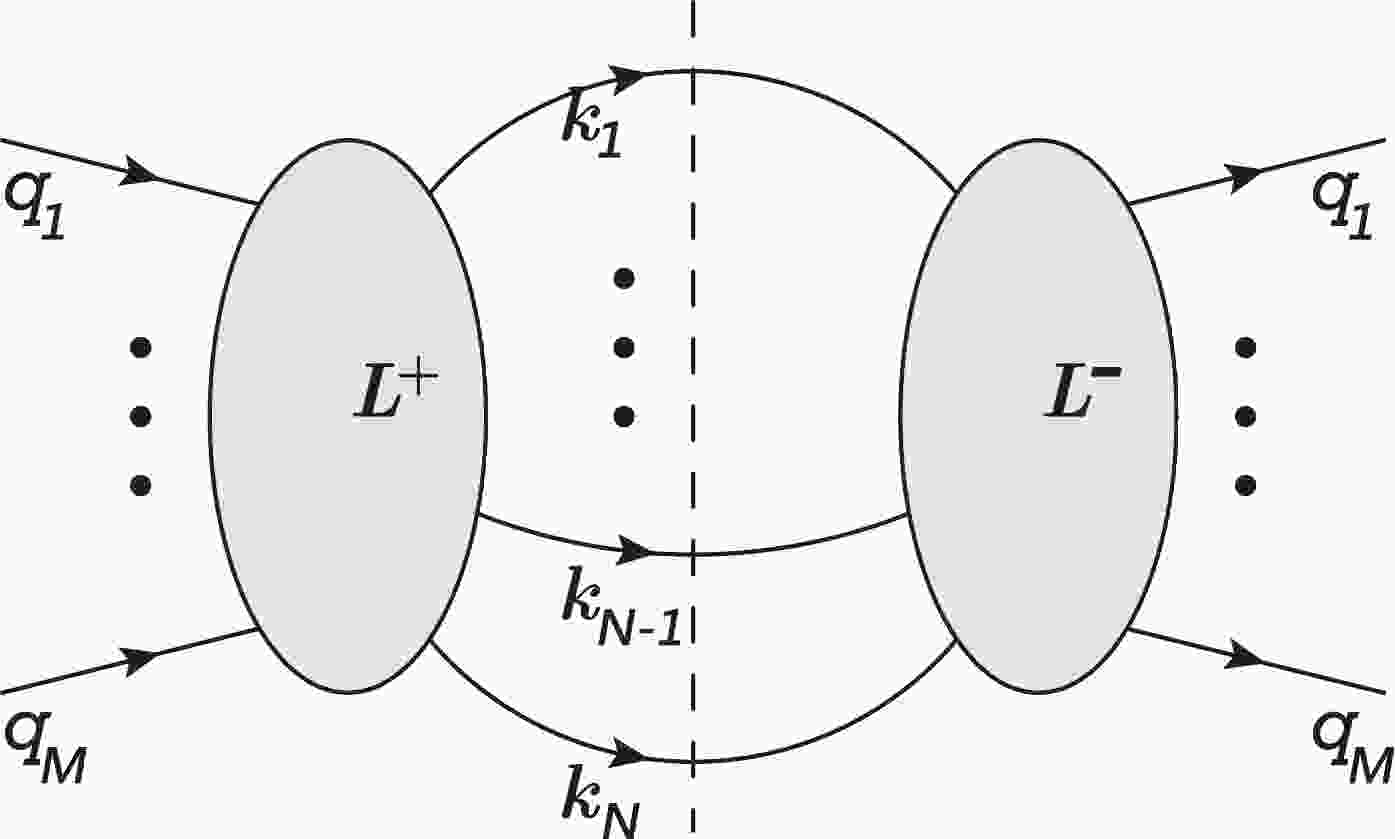
where ${\cal{D}}^{\rm{c}}_i = k_i^2-m_i^2$ can be interpreted either as a mass shell condition or as an inverse propagator on the cut. In this way, techniques developed for calculating loop integration can be used, such as integration-by-parts (IBP) relations [22], differential equations (DEs) [23, 24], dimensional recurrence relations [25-27], and also methods developed by introducing auxiliary mass (AM) [28-34]. Furthermore, loop integration and phase-space integration can be dealt with as a whole because they are not significantly different from each other for these techniques.

To be definite, a schematic cut diagram for a general process is shown in Fig. 1, where $L^+$ is the number of loop momenta (denoted as $\{l_i^+\}$) on the l.h.s. of the cut, $L^-$ is the number of loop momenta (denoted as $\{l_i^-\}$) on the r.h.s. of the cut, $L = L^++L^-$ is the total number of loop momenta, M is the number of external momenta (denoted as $\{q_i\}$) which contains not only initial state external momenta but also fixed and unintegrated final state momenta, and N is the number of cut momenta (denoted as $\{k_i\}$) which are on mass shell, with $m_i$ being the corresponding particle masses. $L^+\geqslant 0$, $L^-\geqslant 0$, $M\geqslant 1$ and $N\geqslant 1$ are reasonable. We denote Q as the total cut momentumwhich satisfies $Q = \displaystyle\sum\limits_{i = 1}^M q_i = \displaystyle\sum\limits_{i = 1}^N k_i$ if $\{q_i\}$ are labeled to flow into the diagram and $\{k_i\}$ flow out of the diagram. A complete set of kinematical invariants after performing loop integration and phase-space integration is denoted as $\vec {s\,}$ , with $Q^2$ as a special component.

Figure 1.  Schematic diagram for a process with $L = L^++L^-$ loops, M unintegrated external legs, and N cut legs.

A general phase-space and loop integration with AM to be studied in this work is

where the non-integer spacetime dimension $D = 4-2\epsilon$ is introduced to regularize all possible divergences, ${\cal{D}}^{ \rm{t}}_{\alpha}$ are the inverse of tree propagators which do not depend on loop momenta, ${\cal{D}}^+_{\alpha}$ are the inverse of loop propagators on the l.h.s. of the cut which do not depend on loop momenta on the r.h.s. of the cut, ${\cal{D}}^-_{\alpha}$ are the inverse of loop propagators on the r.h.s. of the cut which do not depend on loop momenta on the l.h.s. of the cut, the vector $\vec{\nu}\equiv({\nu}^{ \rm{t}}_1, {\nu}^{ \rm{t}}_2,\cdots, {\nu}^+_1,{\nu}^+_2,\cdots,{\nu}^-_1,{\nu}^-_2,\cdots,\nu^{\pm}_{11},\nu^{\pm}_{12},\nu^{\pm}_{21},\cdots)$ with $\nu_{ij}^\pm\leqslant 0$, the vector $\vec{\eta}\equiv({\eta}^{ \rm{t}}_1,{\eta}^{ \rm{t}}_2,\cdots,{\eta}^+_1,{\eta}^+_2,\cdots,{\eta}^-_1,{\eta}^-_2,\cdots)$ denotes the introduced AM terms, and ${\rm{ dPS}}_N$ is the measure of N-particle-cut phase-space integration. For the total cross section, we have

where $\Theta$ is the Heaviside function.^① Differential cross sections can be obtained by introducing constraints into ${\rm{ dPS}}_N$, e.g. an introduction of $\delta(y-k_i\cdot p_1/k_i\cdot p_2)$ can give rise to the rapidity distribution of the i-th particle [20, 21], where $p_1$ and $p_2$ are the momenta of initial-state particles.

The corresponding physical integral can be obtained from the above modified integral by taking all AMs to zero,

It is reasonable to take $\eta^+_\alpha$ and $\eta^-_\alpha$ to zero from the positive side of their real parts, because this is exactly the rule of Feynman prescription for Feynman propagators which guarantees the correct discontinuity of Feynman propagators. For $\eta^{ \rm{t}}_\alpha$, we can take them to zero from any direction as far as all tree propagators are either positive-definite or negative-definite. Our choice is to take all $\eta^{ \rm{t}}_\alpha$ to zero from the positive side so that tree propagators on the l.h.s. of the cut can be combined with the same propagators on the r.h.s. of the cut.^②

For our purpose, we can choose components of $\vec \eta$ to be either fully related to each others or completely independent. One extreme is to choose all the components of $\vec \eta$ to be the same, and the opposite extreme is to choose a strong ordering for all components of $\vec \eta$. Although all these choices are workable, to be definite in this work we assume that components of $\vec \eta$ can only be either $0^+$ or $\eta$. In this way, F only depends on one AM $\eta$, and we denote it as ${F}(\vec{\nu}; \vec s, \eta)$ in the rest of this paper.

In this work, we study the calculation of physical ${F}(\vec{\nu};\vec s,0)$ based on the auxiliary-mass-flow (AMF) method originally proposed in Ref. [28] for pure loop integration, where flow of $\eta$ from $\infty$ to $0^+$ is obtained by solving DEs w.r.t. $\eta$ . We will see that this method is not only systematic and efficient, but can also give high-precision results. The rest of the paper is organized as follows. In Sec. II, we describe the general strategy to calculate integrals involving both loop integration and phase-space integration. In Sec. III, the method is explained in detail using the pedagogical example $e^+e^-\rightarrow \gamma^* \rightarrow t\bar{t}+X$ at NNLO. We also verify the correctness of our calculation by various methods. Finally, a summary is given in Sec. IV. The calculation of basal phase-space integration without a denominator in the integrand is given in Appendix A.

The advantage of introducing $\eta$ is that, by taking $\eta\to \infty$, ${F}(\vec{\nu};\vec s, \eta)$ can be reduced to linear combinations of simpler integrals. As scalar products among external momenta and cut momenta are finite, we have the auxiliary mass expansion (AME) for tree propagators

which removes a tree propagator from the denominator if $\eta$ has been introduced to it. Because loop momenta can be any large value, one cannot naively expand loop propagators in the same way as tree propagators. However,the standard rules of large-mass expansion [35, 36] imply that, as $\eta\to\infty$, linear combinations of loop momenta can be either at the order of ${|\eta|}^{1/2}$ or much smaller than it. Therefore one can perform the following AME,

where we decompose ${\cal{D}}^+_\alpha = \widetilde{{\cal{D}}}^+_{\alpha}+K_\alpha$ with $\widetilde{{\cal{D}}}^+_{\alpha}$ including only the part at the order of ${|\eta|}$. Similarly, we can do the expansion for loop propagators on the r.h.s. of the cut. The AME of loop propagators either removes some propagators from the denominator (if $\eta$ presents in the propagator and $\widetilde{{\cal{D}}}^+_{\alpha} = 0$) or decouples some loop momenta at the order of ${|\eta|}^{1/2}$ from kinematical invariants. The latter effect results in some single-scale vacuum integrals being multiplied by integrals with fewer loop momenta.

We find that, as $\eta\to \infty$, ${F}(\vec{\nu};\vec s, \eta)$ is simplified to a linear combination of integrals with fewer inverse propagators in the denominator (maybe multiplied by single-scale vacuum integrals). If the simplified integrals still have inverse propagators in the denominator (except propagators in single-scale vacuum integrals), we can again introduce new AM $\eta$ and take $\eta\to \infty$. Eventually, ${F}(\vec{\nu};\vec s, \eta)$ is translated to the following form

where c are rational functions of $\vec {s\,}$ and $\eta$, $F^{\rm{bub}}$ includes only single-scale vacuum bubble integrals, and $F^{\rm{cut}}$ denotes basal phase-space integrations with the integrands being polynomials of scalar products between cut momenta. $F^{\rm{bub}}$ have been well studied up to five-loop order (see Refs. [37-43] and references therein). $F^{\rm{cut}}$ can easily be dealt with because the only nontrivial information is the cut propagators, which will be explicitly studied in Appendix A. With this information in hand, the next question is how to obtain physical integrals.

It was shown in Ref. [44] that, for any given problem, Feynman loop integrals form a finite-dimensional vector space, the basis of which is master integrals (MIs). The step to express all loop integrals as linear combinations of MIs is called reduction. With the reverse unitarity relation in Eq. (1), one can map phase-space integrations onto corresponding loop integrations. Therefore, integrals over the phase-space and loop momenta defined in Eq. (2) can also be reduced to corresponding MIs.

Reduction of a general integral to MIs can traditionally be achieved by using IBP relations based on Laporta's algorithm [45-50]. Alternatively, one can achieve IBP reduction using finite-field interpolation [51-56], module intersection [57], intersection theory [58], or AME [29].^③ In any case, the search algorithm proposed in Refs. [29, 32] can significantly improve the efficiency of reduction, which makes the reduction of very complicated problems a possibility. Reduction can not only express all integrals in terms of MIs, it can also set up DEs among MIs [23, 24, 59-62]. Especially, DEs w.r.t. the AM $\eta$ are given by

where $\vec{J}(\vec s, \eta)\equiv \left\{ {F}(\vec{\nu}', \vec s, \eta), {F}(\vec{\nu}'', \vec s, \eta), \cdots\right\}$ is a complete set of MIs and $M(\vec s, \eta)$ is the coefficient matrix as a rational function of $\vec s$ and $\eta$. The boundary condition of the DEs can be chosen at $\eta\to\infty$, which can easily be obtained by the AME discussed above. By solving the above DEs (usually numerically) one can realize the flow of $\eta$ from $\infty$ to $0^+$. In this way, we get a general method to calculate physical MIs $\vec{J}(\vec s, 0)$ with any fixed $\vec s$.

Furthermore, in the case of more than one kinematical invariant, the AMF method can also be combined with DEs w.r.t. $\vec{s}$ to obtain MIs at different values of $\vec{s}$.

We emphasize that, in practice, one should first reduce the scattering amplitude to MIs without AM, and then calculate these MIs by introducing AM. Therefore, the AMF method does not change the step of reducing scattering amplitude. It does make the step of setting up DEs w.r.t. AM $\eta$ more complicated than the traditional DE method because one more scale is involved. However, the cost is always tolerable as it is still simpler than the step of reducing full scattering amplitude.

As a simple but nontrivial example, we calculate the MIs encountered in the NNLO correction for $t\bar{t}$ production in an $e^+ e^-$ collision mediated by a virtual photon to demonstrate the validity of the AMF method. For the purpose of total cross section, there are only two kinematical invariants ($Q^2$ and $m_t^2$) besides $\eta$. Thus we can introduce dimensionless integrals

where $s = Q^2$, $x = \dfrac{4m_t^2}{s}$, $y = \dfrac{\eta}{s}$ and $\nu$ is the summation of all components of $\vec \nu$. Because the problem is simple, we make the following unoptimized scheme choice:

with $\eta_1^{ \rm{t}}\ll \eta_1^+$. More precisely, if $\{{\cal{D}}^-_{\alpha}\}$ or $\{{\cal{D}}^+_{\alpha}\}$ depends on $\vec {s\,}$, we choose $\eta^{ \rm{t}}_1 = 0^+$ and $\eta^+_1 = \eta$; otherwise, we choose $\eta^{ \rm{t}}_1 = \eta$ (the introduction of $\eta_1^+$ is unnecessary in this case). The publicly available systematic package FIRE6 [47] is sufficient to do all needed reductions in this simple exercise.

There are many subprocesses at the partonic level. We use ${\rm{V}}^{L^+}{\rm{R}}^{N-1}{\rm{V}}^{L^-}$ to distinguish processes with different numbers of independent loop momenta and cut momenta. The presence of $N-1$ instead of N is a result of momentum conservation, which reduces one independent cut momentum. For completeness, we first provide MIs at NLO in Sec. III A. The calculation of MIs for 4-particle cuts at NNLO (RRR) is presented in Sec. III B. The calculation of MIs for 3-particle cuts at NNLO (VRR) is presented in Sec. III C, and the calculation of MIs for 2-particle cuts at NNLO (VVR or VRV) is presented in Sec. III D. Verification of these results is given in Sec. III E. We note that all these results have already been calculated in the literature using other methods (see, e.g., Refs. [63-66]) although they are not fully publicly available. We provide our results as ancillary file with the arXiv version of this paper.

For RR, i.e. the $\gamma^*\to t\bar{t}g$ process, the inverse propagators can be written as

The 2 physical MIs obtained are $F^{\rm{cut}}_{2,3,1}$ and $F^{\rm{cut}}_{2,3,2}$, which are calculated in Appendix A.

For VR, the inverse propagators can be written as

We obtain 1 family^④ with $\vec \nu$ of the characterized MIs being $\{1,1,0\}$. Physical MIs are given by

where $\Phi_2 = \int{\rm{dPS}}_2$ is defined in Eq. (A5) and the remaining 1-loop integrals are easy to calculate analytically.

For RRR, i.e., $\gamma^*\to t\bar{t}gg$ or $t\bar{t} q\bar{q}$ processes, the inverse propagators can be written as

where $Q^2 = s$. The phase-space integrals can then be expressed as

Using FIRE6, we find that there are 37 MIs for finite $\eta$ and the number is reduced to 15 as $\eta$ vanishing.^⑤ These MIs can be classified into 2 families, with $\vec \nu$ of the characterized MIs being

which can also characterized by Feynman diagrams Fig. 2(a) and (b), respectively. Using our method, we can calculate all physical MIs with any fixed x. The result of the most complicated MI with e.g. $x = 1/2$ is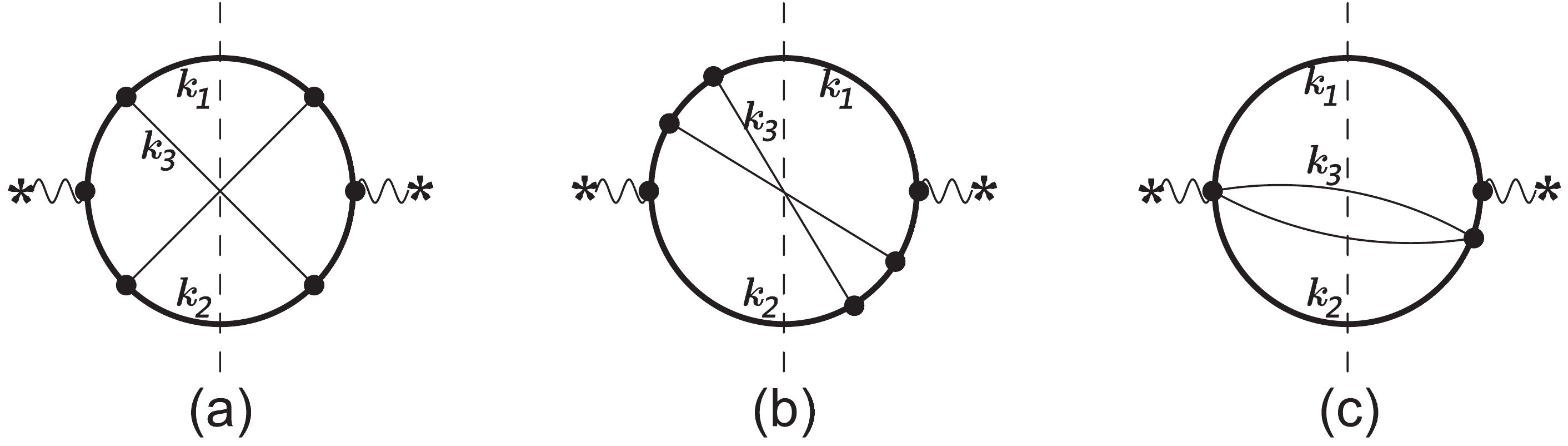

Figure 2.  Representative Feynman diagrams for $\gamma^*\rightarrow t\bar{t}gg$ or $t\bar{t} q\bar{q}$ processes, where (a) and (b) define the two most complicated families and (c) defines a sub-family of (b). The thick curves represent top quarks, the thin curves represent massless particles, and the vertical dashed lines represent the final state cut.

where we truncate the expansion to order $\epsilon^8$ with about 30-digit precision for each coefficient. Physical MIs with other values of x can be calculated similarly.

In the following, let us take a sub-family $\{0,0,0,0,0,0,1\}$, shown in Fig. 2(c) , as an example to illustrate the calculation procedure for MIs. For brevity, we define the MIs for this family as:

with $\nu^{ \rm{t}}_1, \nu^{ \rm{t}}_2\leqslant 0$ and $\nu^{ \rm{t}}_7\geqslant 0$. This family contains 5 MIs for finite $\eta$ (or y)

and 4 MIs as $\eta\to0^+$

It is clear that the first three MIs of the two sets are just linear combinations of $F^{\rm{cut}}$ that have been calculated in Appendix A.

To calculate the last physical MI in Eq. (22), we set up DEs for corresponding MIs with $x = 1/2$ and finite $\eta$, which gives

The boundary condition of these DEs is given by

By solving the DEs (23) with the boundary condition we obtain, e.g.,

　　Finally, the DE w.r.t. x is given by

With the boundary condition at $x = 1/2$ given in Eq. (25), solving the above DE can also give $\hat F(\{0,0,1\};x,0)$ at any value of x.

For VRR, the inverse propagators can be written as

where $Q^2 = s$. Then the 1-loop $1\to3$ phase-space integrals can be expressed as

We find that there are 71 MIs for finite $\eta$ (or y) and the number is reduced to 27 when $\eta\to 0^+$. These MIs can be classified into 2 families,

The first family is the most complicated. It can also be characterized by the Feynman diagram in Fig. 3(a). Using our method, the result of the most complicated MI with, e.g., $x = 1/2$ is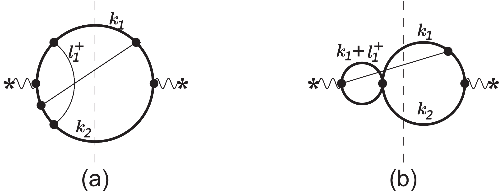

Figure 3.  Representative Feynman diagrams in VRR, where (a) defines the most complicated family and (b) defines a sub-family of (a). The thick curves represent top quarks, the thin curves represent massless particles, and the vertical dashed lines represent the final state cut.

In the following, let us take a sub-family $\{1,0,1,1,0,0,0,0\}$ , shown in Fig. 3(b) , as an example to illustrate the calculation procedure for MIs. For brevity, we define the MIs for this family as:

This family contains 7 MIs for finite $\eta$

and 6 MIs as $\eta\to0^+$

　　To calculate the last 2 physical MIs, we set up DEs for corresponding MIs with $x = 1/2$ and finite $\eta$, which gives

The boundary condition for these DEs is given by

where

and $\int{\rm{dPS}}_3\dfrac{1}{{\cal{D}}^ {\rm{t}}_1}$ can again be calculated by the method inSec. III B or obtained from RR in Sec. III A. Knowing the first 5 MIs, by solving the DEs (34) with the boundary condition we obtain e.g.,

　　Finally, the DEs w.r.t. x are given by

With the boundary condition at $x = 1/2$ given in Eq. (37), by solving the above DEs we can also evaluate $\hat F(\{1,1,1\};x,0)$ and $\hat F(\{1,1,2\};x,0)$ at any value of x.

For VVR, the inverse propagators can be written as

Then the phase-space integrals can be expressed as

We find that there are 53 MIs for finite $\eta$ and the number is reduced to 21 when $\eta\to 0^+$. These MIs can be classified into 3 families

The first family is the most complicated. It can be characterized by the Feynman diagram in Fig. 4(a). We use the same method (note, $F^{\rm{bub}}$ up to 2-loop is needed to calculate boundary conditions) in VRR to calculate MIs for these families.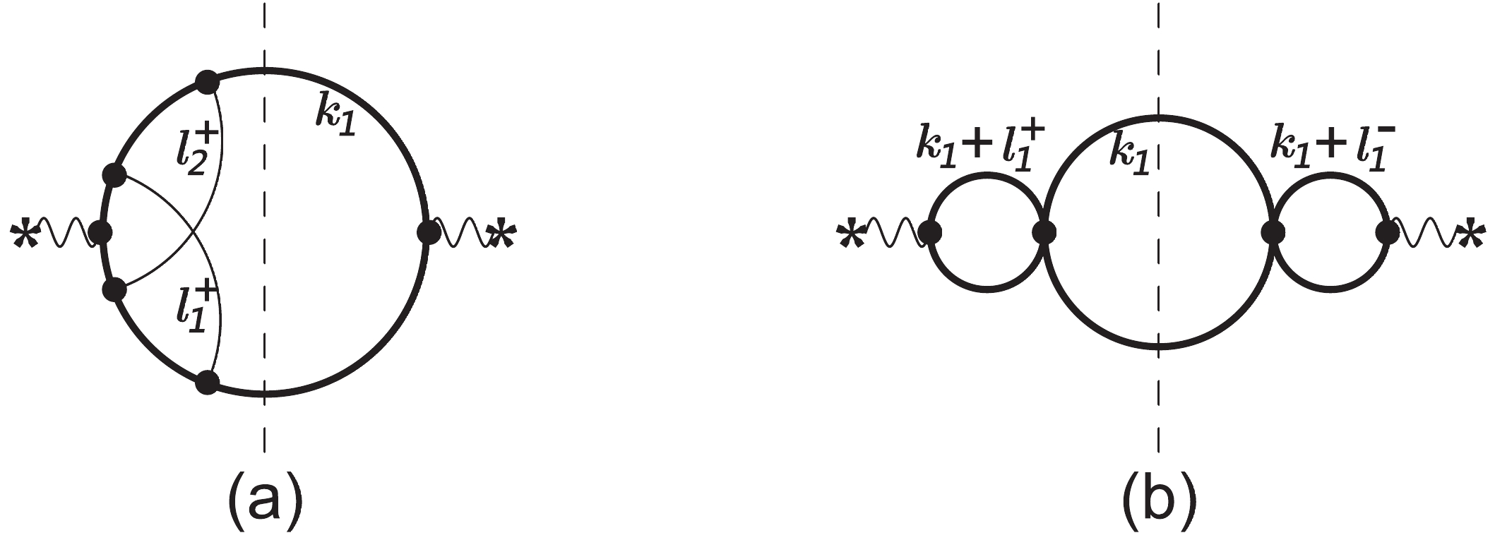

Figure 4.  Representative Feynman diagrams in VVR and VRV, where (a) defines the most complicated family for VVR and (b) defines the family for VRV. The thick curves represent top quarks, the thin curves represent massless particles, and the vertical dashed lines represent the final state cut.

For VRV, the inverse propagators can be written as

in addition to which there is a scalar product $l_1^+\cdot l_1^-$. The obtained family is:

which can also be characterized by the Feynman diagram Fig. 4(b). Because loop integrations in MIs of this case are factorized, their calculation is as simple as the one-loop case.

On the one hand, the AMF method can be used to calculate MIs at any given value of x. On the other hand, MIs at different values of x can be related by DEs w.r.t. x. We have verified that the results of MIs obtained by the two strategies for different values of x, e.g., $x = 1/2$ and $x = 2/5$, are consistent with each other. This provides a highly nontrivial self-consistency check because DEs w.r.t. $\eta$ and w.r.t. x are significantly different.

Our numerical values for $\hat F(\vec{\nu};0,0)$, i.e. MIs for massless QCD, are in full agreement with the known analytical results of massless MIs in the literature [67, 68].

For the RRR sub-process (Sec. III B), our numerical results for $\hat F(\{0,0,0,0,0,0,1\};x,0)$ and $\hat F(\{0,0,0,1,0,0,1\}; x,0)$ show excellent agreement with the corresponding analytical results in the literature [63] ($T_4$ and $T_5$ in this reference).

In this paper, we have extended the AMF method originally developed for Feynman loop integrals [28] to calculate MIs which also involve phase-space integration. As a pedagogical example, we used this method to calculate the MIs encountered in $e^+e^-\rightarrow \gamma^* \rightarrow t\bar{t}+X$ at NNLO. Our results agree with results obtained by using other methods (our full results are available as an ancillary file with the arXiv version of this paper). Although the AMF method depends on a reduction procedure to decompose all integrals to MIs and to set up the DEs of MIs w.r.t. $\eta$, the efficiency of reduction has been significantly improved thanks to the recently proposed search algorithm [29, 32].

It is clear that the AMF method can be used to calculate MIs of any process, as systematically as the sector decomposition method. However, compared with the latter method, the AMF method is much more efficient and can provide very high precision. Its high-precision nature makes it possible to obtain analytical results with a proper ansatz. For problems with two or more kinematical invariants, where the DE method works, the AMF method can not only systematically provide as many boundary conditions as needed for DEs w.r.t. kinematical invariants, but also provides a highly nontrivial self-consistency check for the obtained results. All the above advantages make the AMF method very useful for perturbative calculation at high orders.

We thank Chen-Yu Wang, K.T. Chao and C. Meng, Xin Guan, Xiao-Bo Jin, Zhi-Feng Liu for many helpful communications and discussions.

In this appendix, we calculate the MIs of basal phase-space integration with no denominator. It is important to note that, besides the masses presented in cut lines, these MIs only depend on the square of the center of mass energy $s\equiv Q^2$, regardless of the configuration of external unintegrated momenta. We use $F_{r,N,n}^{\rm{cut}}$ to denote the n-th MI for N-particle-cut integrals with $m_1 = \cdots = m_r = m$ and $m_{r+1} = \cdots = m_N = 0$, and we provide explicit results for $r = 0,\; 1$, and $2$. MIs for general cases can be studied as follows. By using the optical theorem (see e.g. Ref. [67]), the calculation of the basal phase-space integral is translated to the calculation of the imaginary part of the corresponding sunrise pure loop integral. The latter can be calculated by the AMF method for loop integrals [28]. Furthermore, a one-dimensional-integral representation of all these MIs can be obtained from Ref. [69].

For $r = 0$ and $N\geqslant 2$, there is only one MI, which is given by

For $r = 1$, in general there are two MIs, which are given by ($n = 1,2$)

where ${}_pF_q$ are generalized hypergeometric functions which can be evaluated using the publicly available program HypExp [70]. In the special case of $N = 2$, there is only one MI $F^{\rm{cut}}_{1,2,1}$. For $r = 2$, in general there are three MIs, which are given by ($n = 1,2,3$)

In the special case of $N = 2$, there is only one MI, which means $F^{\rm{cut}}_{2,2,2}$ and $F^{\rm{cut}}_{2,2,3}$ can be reduced to $F^{\rm{cut}}_{2,2,1}$. In the special case of $N = 3$, there are only two MIs, which means $F^{\rm{cut}}_{2,3,3}$ can be reduced to $F^{\rm{cut}}_{2,3,1}$ and $F^{\rm{cut}}_{2,3,2}$. The number of MIs obtained here is consistent with the expectation in Ref. [71]. The results (A2) and (A3) agree with the partial results in the literature (see Eq. (B.7) in Ref. [72] and Eqs. (3.14-3.16) in Ref. [63]).

To obtain Eqs. (A2) and (A3), we decompose the measure of phase-space integration into two parts:

where $\Omega$ is a subset of $\{1,2,\cdots,N\}$ and $\#_{\Omega}$ is the number of elements of $\Omega$. Specifically, $\Omega$ is chosen to be the set of massless particles for $r = 1$, and is chosen to be the set of massive particles for $r = 2$. The phase-space volume of the two-particle cut is used:

The following relations (which can be found from e.g. Ref. [73]) are also useful: