Instability of regularized 4D charged Einstein-Gauss-Bonnet de-Sitter black holes

I. INTRODUCTION

• I. INTRODUCTION
• II. THE 4D CHARGED EGB-DS BLACK HOLE
• III. THE CHARGED SCALAR PERTURBATION
• IV. THE INSTABILITY OF THE 4D CHARGED EGB-DS BLACK HOLE
•      A The asymptotic iteration method (AIM)
•      B The eigenfrequencies of the charged scalar perturbation
•      C Evolution of the perturbation field
•      D Effective potential
• V. SUMMARY AND DISCUSSION
• ACKNOWLEDGMENTS

It is known that general relativity should be modified from the viewpoints of both theory and observations. For example, general relativity cannot be renormalized and cannot explain the dark side of the universe. In contrast, the Lovelock theorem states that, in the four dimensional vacuum spacetime, general relativity with the cosmological constant is a unique metric theory of gravity with second order equations of motion and covariant divergence-free [1]. Beyond general relativity, one must consider higher dimensional spacetimes, add extra fields, allow higher order derivatives of metrics, or even abandon the Riemannian geometry. Various modified gravity theories have been proposed [2].

By rescaling the GB coupling constant in a special way, a regularized 4D GB black hole solution was found recently [3]. This work provides a novel classical 4D gravity theory and has inspired many studies, including those on regularized black hole solutions [4-23], perturbations [24-35], shadow and geodesics [36-41]， thermodynamics [42-47], and other aspects [48-51]. It should be mentioned that 4D EGB gravity was found to be inconsistent based on the theory proposed in [3]. Fortunately, some proposals have been raised to circumvent the issues of 4D EGB gravity, including adding an extra degree of freedom to the theory [18-23] or breaking the temporal diffeomorphism invariance [52, 53], where a well-defined theory was formulated. In contrast, while the 4D EGB gravity formulated in [3] may be problematic at the level of action or equations of motion, the spherically symmetric black hole solution derived in [3] can be obtained from conformal anomalyand quantum corrections [54-65] as well as from the Horndeski theory [18-23], which means the spherically symmetric black hole solution itself is meaningful and worth studying.

The regularized black hole solution has some remarkable properties. Its singularity at the center is timelike. The gravitational force near the center is repulsive, and the free infalling particles cannot reach the singularity [3]. One may expect that the regularized black hole solution would also show some novel properties with respect to perturbations, and some related studies have been reported [24-32, 34]. The study of the stability of black holes is an active area in black hole physics. It can be used for extracting the black hole parameters such as its mass, charge, and angular momentum. Black hole stability is also related to gravitational waves, black hole thermodynamics, the information paradox, and holography [57, 58]. Among these studies, black hole stability in the asymptotic de Sitter (dS) spacetime is intriguing. For example, spontaneous scalarization of Kerr-dS black holes in the scalar-tensor theory behaves very differently from that for asymptotically flat spacetimes under perturbations [59]. The 4D Reissner-Nordström-de Sitter (RN-dS) black hole may violate strong cosmic censorship [60-63]. Higher dimensional RN-dS and Gauss-Bonnet-de Sitter (GB-dS) black holes are unstable [64-68].

A quite surprising and still not very well understood result was discovered in [69-71], where it was shownthat the RN-dS black hole is unstable under charged scalar perturbations. Such instability satisfies the superradiancecondition [72]. However, only the monopole $l = 0$ suffers from this instability. Higher multipoles are stable. This is distinct from superradiance. The underlying mechanismmay be understood using the tools of nonlinear analysis, as was partially shown recently [63]. In this paper, we consider the instability of the regularized 4D charged EGB black hole in the asymptotic dS spacetime, under charged scalar perturbations. We demonstrate that the behavior is very different from the case of the asymptotic flat spacetime that was considered in [34]. The GB coupling constant plays a more subtle role here.

The paper is organized as follows. Sec. II describes the regularized 4D EGB-RN-dS black hole and gives a reasonable parametric region. Sec. III presents the charged scalar perturbation equations. Sec. IV describes the numerical method we used and presents the results for quasinormal modes (QNMs). Sec. V contains the summary and discussion of the study.

II. THE 4D CHARGED EGB-DS BLACK HOLE

• I. INTRODUCTION
• II. THE 4D CHARGED EGB-DS BLACK HOLE
• III. THE CHARGED SCALAR PERTURBATION
• IV. THE INSTABILITY OF THE 4D CHARGED EGB-DS BLACK HOLE
•      A The asymptotic iteration method (AIM)
•      B The eigenfrequencies of the charged scalar perturbation
•      C Evolution of the perturbation field
•      D Effective potential
• V. SUMMARY AND DISCUSSION
• ACKNOWLEDGMENTS

The 4D spherical symmetric EGB black hole in the electrovacuum dS spacetime can be written as [4]

where the metric function is

and the gauge potential is

Here, M is the black hole mass, Q is the black hole charge, and $\Lambda$ the positive cosmological constant. When $\alpha\to0$, this solution converges to that for the RN-dS black hole. As $r\to\infty$, the asymptotic dS spacetime with an effective positive cosmological constant is obtained. Note that solution (1) coincides formally with those obtained from the Horndeski theory [18-23] and those obtained using conformal anomaly and quantum corrections [52, 53].

The GB coupling constant $\alpha$ can be either positive or negative. In an appropriate parametric region, the solution has three horizons: the inner horizon $r_{-}$, the event horizon $r_{+}$, and the cosmological horizon $r_{c}$. For negative $\alpha$, the metric function may not be real in the small r region. However, since we are only interested in the region between $r_{+}$ and $r_{c}$, we allow negative $\alpha$ in this work. For convenience, hereafter, we fix the black hole event horizon as $r_{+} = 1$. Then, the mass parameter can be expressed as

Note that, to ensure $f(1) = 0$, we must have $\alpha>-\frac{1}{2}$. The parametric region in which the black hole event horizon $r_{+}$ and the cosmological horizon $r_{c}$ are allowed can be determined by requiring $f'(r_{+})>0$, implying that the black hole temperature is positive. This leads to

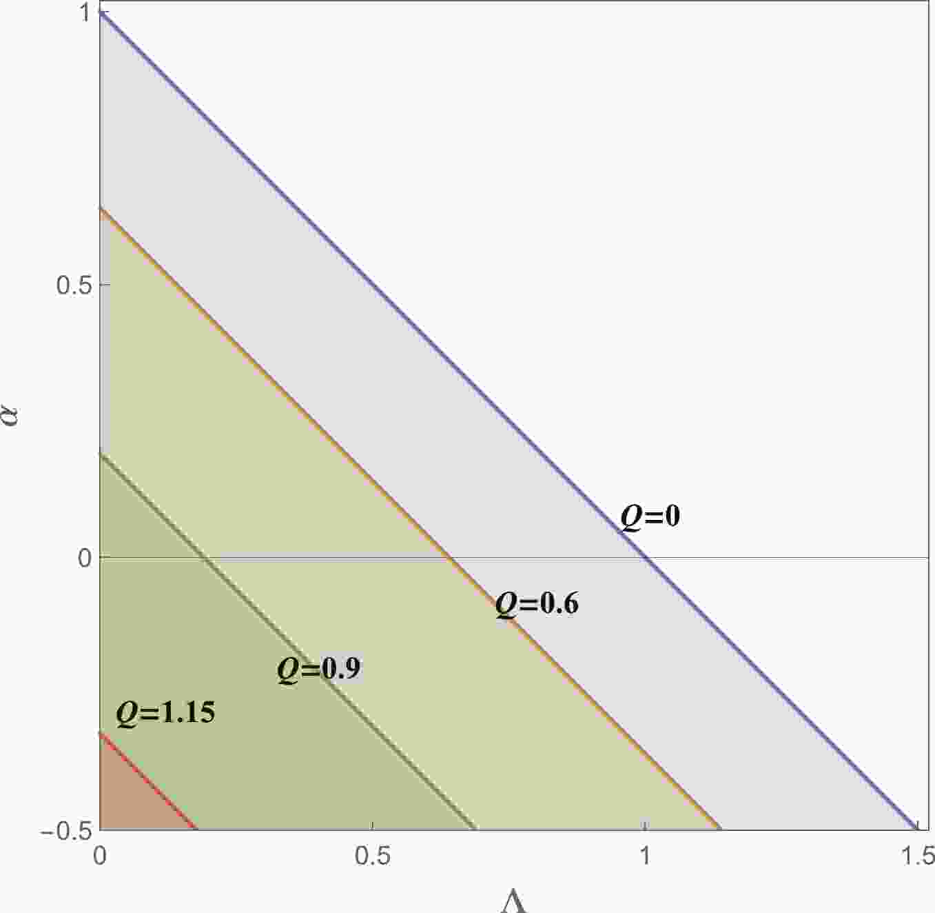
This formula is very similar to the neutral case [33]. The parametric region is shown in Fig. 1.

Figure 1

Figure 1.  (color online) The parametric region that allows the event horizon $r_{+}$ and cosmological horizon $r_{c}$. The region is bounded by $Q^{2}+\alpha+\Lambda<1,$ $-0.5<\alpha$, $\Lambda>0$, and $Q>0$. As Q increases, the allowed region for $(\Lambda,\alpha)$ shrinks. The extremal value of $Q = \sqrt{3/2}$.

DownLoad: Full-Size Img PowerPoint

III. THE CHARGED SCALAR PERTURBATION

• I. INTRODUCTION
• II. THE 4D CHARGED EGB-DS BLACK HOLE
• III. THE CHARGED SCALAR PERTURBATION
• IV. THE INSTABILITY OF THE 4D CHARGED EGB-DS BLACK HOLE
•      A The asymptotic iteration method (AIM)
•      B The eigenfrequencies of the charged scalar perturbation
•      C Evolution of the perturbation field
•      D Effective potential
• V. SUMMARY AND DISCUSSION
• ACKNOWLEDGMENTS

It is known that fluctuations of order ${\cal{O}}(\epsilon)$ in the scalar field in a given background induce changes in the spacetime geometry of order ${\cal{O}}(\epsilon^{2})$ [72]. To the leading order, we can study perturbations for a fixed background geometry. Let us consider a massless charged scalar field $\psi$ on background (1). Its equation of motion is

where q is the scalar charge, and $\nabla_{\mu}$ is the covariant derivative. For a generic background, we can take the following decomposition

Here, $Y_{lm}(\theta,\phi)$ is the spherical harmonics on the two sphere $S^{2}.$ The angular part and the radial part of the perturbation Eq. (6) decouple. What we are interested in is the radial part, which can be written in the Schrödinger-like form

where the tortoise coordinate ${\rm d}r_{\ast} = {\rm d}r/f$ is introduced. The effective potential reads

Unlike the case of the asymptotic flat spacetime, where only one potential barrier appears between $r_{+}$ and $r_{c}$, here, a negative effective potential well may appear between $r_{+}$ and $r_{c}$. We will show that this potential well plays an important role in the instability of charged EGB-dS black holes under perturbations.

The radial equation exhibits the following asymptotic behavior near the horizons.

Here, $\kappa_{+} = \dfrac{1}{2f'(r_{+})}$ is the surface gravity on the event horizon, and $\kappa_{c} = -\dfrac{1}{2f'(r_{c})}$ is the surface gravity on the cosmological horizon. Thisasymptotic solution corresponds to the ingoing boundary condition near the event horizon and outgoing boundary condition near the cosmological horizon. The system is dissipative, and the frequency of perturbations is determined by the composition of QNMs. For a specific boundary condition (10), the radial Eq. (8) can be solved as an eigenvalue problem. Only some discrete eigenfrequencies $\omega$ satisfy both the radial equation and the boundary condition. The eigenfrequency can be written as $\omega = \omega_{\rm R}+{\rm i}\omega_{\rm I}$. When the imaginary part $\omega_{\rm I}>0$, the amplitude of the perturbationwill increase exponentially, implying that the black hole is unstable at least with respect to linear perturbations.

IV. THE INSTABILITY OF THE 4D CHARGED EGB-DS BLACK HOLE

• I. INTRODUCTION
• II. THE 4D CHARGED EGB-DS BLACK HOLE
• III. THE CHARGED SCALAR PERTURBATION
• IV. THE INSTABILITY OF THE 4D CHARGED EGB-DS BLACK HOLE
•      A The asymptotic iteration method (AIM)
•      B The eigenfrequencies of the charged scalar perturbation
•      C Evolution of the perturbation field
•      D Effective potential
• V. SUMMARY AND DISCUSSION
• ACKNOWLEDGMENTS

The radial Eq. (8) with boundary conditions specified by (10) is generally difficult to solve analytically, except for a few cases, such as the pure anti-dS ((A)dS) spacetime, the Nariai spacetime, and massless topological black holes [57, 58]. In general, approximations or numerical methods are required. Various numerical methods for QNM calculations have been developed, such as the Wentzel-Kramers-Brillouin (WKB) method, the shooting method, the continued fraction method, and the Horowitz-Hubeny method [57, 58]. Not all of these methods have high accuracy and efficiency in the charged case [73]. In this work, we adopted the asymptotic iteration method [74, 75]. In addition, we validate our results using asymptotic iteration methods with time evolution.

A The asymptotic iteration method (AIM)

• I. INTRODUCTION
• II. THE 4D CHARGED EGB-DS BLACK HOLE
• III. THE CHARGED SCALAR PERTURBATION
• IV. THE INSTABILITY OF THE 4D CHARGED EGB-DS BLACK HOLE
•      A The asymptotic iteration method (AIM)
•      B The eigenfrequencies of the charged scalar perturbation
•      C Evolution of the perturbation field
•      D Effective potential
• V. SUMMARY AND DISCUSSION
• ACKNOWLEDGMENTS

The AIM was originally developed for solving the eigenvalues of homogeneous second order ordinary derivative functions [76, 77]. Later, it was used for observing QNMs of black holes in the asymptotic flat or (A)dS spacetimes [74, 75]. Let us first introduce an auxiliary variable

It ranges from 0 to 1 as r runs from the event horizon to the cosmological horizon. The radial Eq. (8) then becomes

The above equation is in general difficult to solve ana-lytically; thus, we use numerical methods. In terms of $\xi$, the asymptotic solution near the horizons can be written as

Then, we can write the full solution of Eq. (12) satisfying the asymptotic behavior (13), as follows:

Here, $\chi(\xi)$ is a regular function of $\xi$ in the interval $(0,1)$, and it obeys the following homogeneous second order differential equation

in which the coefficients are

The coefficients $\lambda_{0}(\xi)$ and $s_{0}(\xi)$ are regular functions of $\xi$ in the interval $(0,1)$. Differentiating (15) with respect to $\xi$ iteratively leads to an $(n+2)$-th order differential equation

where the coefficients are determined iteratively, as follows:

Expanding the coefficient functions around a regular point $\xi = \xi_0$,

in which the expansion coefficients $c_n^j$ and $d_n^j$ are functions of $\omega$, and the iterative equations give

For sufficiently large n, the cutoff of the iteration in the AIM is given by

which leads to the following expression, in terms of the expansion coefficients:

The QNMs $\omega$ can be worked out by solving this equation. We vary the iteration times and the expansion point to ensure the reliability of the results. The results are also checked by using other auxiliary variables such as $\xi = 1-\dfrac{r_{+}}{r}$ or $\xi = \left(1-\dfrac{r_{+}}{r}\right)/\left(1-\dfrac{r_{+}}{r_{c}}\right)$. Except for some extremal cases ($\Lambda\to0$ or when the bblack hole becomes extremal), they coincide well. Hereafter, we set $q = 1$ for convenience.

B The eigenfrequencies of the charged scalar perturbation

• I. INTRODUCTION
• II. THE 4D CHARGED EGB-DS BLACK HOLE
• III. THE CHARGED SCALAR PERTURBATION
• IV. THE INSTABILITY OF THE 4D CHARGED EGB-DS BLACK HOLE
•      A The asymptotic iteration method (AIM)
•      B The eigenfrequencies of the charged scalar perturbation
•      C Evolution of the perturbation field
•      D Effective potential
• V. SUMMARY AND DISCUSSION
• ACKNOWLEDGMENTS

Let us first study the effects of the black hole charge Q on the fundamental modes of QNMs. The results are shown in Fig. 2. In the left panel, we see that $\omega_{\rm R}$ increases with Q almost linearly. The slope is steeper for larger $\Lambda$ and $\alpha$. In the right panel, $\omega_{\rm I}$ increases for small Q and then decreases for larger Q. For sufficiently large Q, the black hole becomes stable. When Q is small, $\omega_{\rm I}$ increases with increasing $\alpha$. This behavior is similar to the case of the asymptotic flat spacetime [34]. However, when Q is large, $\omega_{\rm I}$ decreases with increasing $\omega_{\rm I}$. This should be contrasted with the result for the asymptotic flat spacetime. It implies that the positive GB coupling constant can destabilize the black hole when the black hole charge Q is small, whereas it stabilizes the black hole at large Q. Note further that, regardless of the values of $\Lambda,\alpha$ considered, when $Q\to0$, both $\omega_{\rm R}$ and $\omega_{\rm I}$ tend to 0 from above. This implies that weakly charged black holes in the dS spacetime are always unstable. The existence of $\alpha$ does not change this phenomenon qualitatively.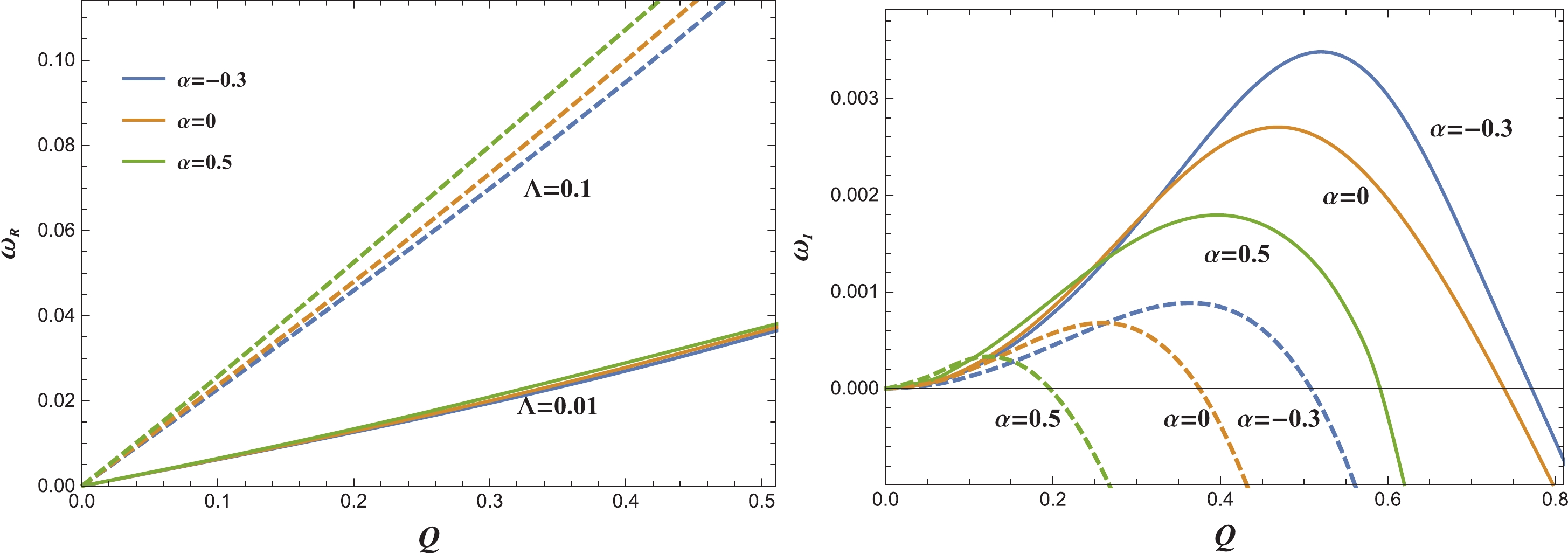

Figure 2

Figure 2.  (color online) The real part (left) and the imaginary part (right) of the fundamental modes of the QNMs, for $l = 0$. The solid lines are for $\Lambda = 0.01$, while the dashed lines are for $\Lambda = 0.1.$

DownLoad: Full-Size Img PowerPoint

Now, we study the effects of $\alpha$ on the fundamental modes in more detail. Fig. 3 shows the real part of the fundamental modes $\omega_{\rm R}$, for $Q = 0.1$ and $Q = 0.4$. For fixed Q, the real part $\omega_{\rm R}$ increases almost linearly with $\alpha$ and $\Lambda$. Combining the results from Fig. 2, we conclude that $\omega_{\rm R}\propto\alpha\Lambda Q$.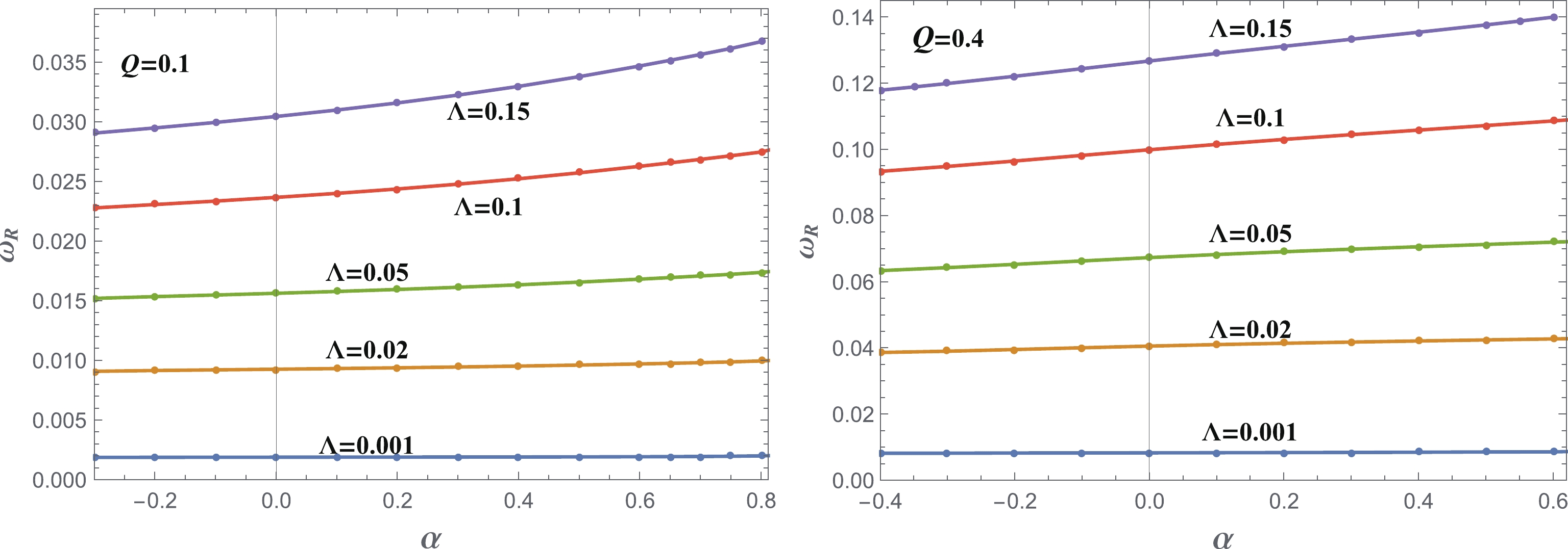

Figure 3

Figure 3.  (color online) The real part of the fundamental modes of the QNMs, for $l = 0$. The left panel is for $Q = 0.1$, while the right panel is for $Q = 0.4$.

DownLoad: Full-Size Img PowerPoint

The behavior of the imaginary part of the fundamental modes $\omega_{\rm I}$ is more interesting. In Fig. 4, we show the cases for $Q = 0.1$ and $Q = 0.4$. From the left and right panels, we see that $\omega_{\rm I}$ increases with small $\Lambda$ and decreases with larger $\Lambda$. The effect of $\alpha$ on $\omega_{\rm I}$ is subtle and relevant to $\Lambda$ and Q. When both Q and $\Lambda$ are small (left upper panel), $\omega_{\rm I}$ increases with $\alpha$. For small Q and larger $\Lambda$ (right upper panel), $\omega_{\rm I}$ increases with $\alpha$ first and then decreases with $\alpha$. For larger Q (lower panels), $\omega_{\rm I}$ decreases with $\alpha$. This phenomenon is very different from the case of the asymptotic flat spacetime [34], where $\alpha$ roughly increases $\omega_{\rm I}$. This implies that the positive GB coupling constant $\alpha$ can suppress the black hole instability. As $\alpha$ increases, it can even change the qualitative behavior of a black hole under a perturbation and can render an unstable black hole stable.

Figure 4

Figure 4.  (color online) The imaginary part of the fundamental modes of the QNMs, for $l = 0$. The upper panel is for $Q = 0.1$, while the lower panel is for $Q = 0.4$. The left panel shows the results for small $\Lambda$, while the right panel shows the results for larger $\Lambda$.

DownLoad: Full-Size Img PowerPoint

The instability we found here is reminiscent of superradiance. However, the present case is quite subtle. Using a method similar to that in [34, 70], one can show that the superradiance occurs only when

Although the unstable modes encountered in our study indeed satisfy (25), it is observed that some oscillation frequencies corresponding to stable modes also are in the range determined by (25) (see Table 1 for evidence). In fact, as shown in [34, 70], the superradiant condition is the necessary but not sufficient condition for instability. The precise mechanism of the instability found here should be studied better and will be addressed in Sec. V.

Table 1

Table 1.  The fundamental modes for $Q = 0.1,\;\Lambda = 0.12$, and $l = 0$, corresponding to the orange line in the upper right panel of Fig. 4. The last column is the imaginary part of the frequency extracted from the time evolution.

$\alpha$	$\dfrac{qQ}{r_{+} }$	$\dfrac{qQ}{r_{c} }$	$\omega$ (AIM)	$\omega_{\rm I}$ (time domain)
0.5	0.1	0.0244042	0.0290311+0.0001514i	0.0001515
0.6	0.1	0.0248557	0.0297114+0.0000779i	0.0000780
0.65	0.1	0.0250987	0.0300692+0.0000191i	0.0000192
0.7	0.1	0.0253547	0.0304355-0.0000541i	-0.0000547
0.75	0.1	0.0256252	0.0308094-0.0001400i	-0.0001390

DownLoad: CSV

Show Table

C Evolution of the perturbation field

• I. INTRODUCTION
• II. THE 4D CHARGED EGB-DS BLACK HOLE
• III. THE CHARGED SCALAR PERTURBATION
• IV. THE INSTABILITY OF THE 4D CHARGED EGB-DS BLACK HOLE
•      A The asymptotic iteration method (AIM)
•      B The eigenfrequencies of the charged scalar perturbation
•      C Evolution of the perturbation field
•      D Effective potential
• V. SUMMARY AND DISCUSSION
• ACKNOWLEDGMENTS

We also directly compute the time-evolution of the perturbation field $\psi$ to further reveal the instability of the 4D charged EGB-dS black hole. For the time evolution, the Schrödinger-like equation becomes

In order to compute the time evolution of $\psi$, we adopt the discretization approach introduced in [69]. The reliability of this numerical method can be verified by the convergence of computations when increasing the sampling density. We impose the following initial profile:

Eq. (26) is discretized in the $(r_*,t)$ plane. In addition, we set $\Delta t/\Delta r_* = 0.5$, to satisfy the von Neumann stability conditions. Unlike some other analytical models where $r_*$ can be solved analytically, here, $r_*(r)$ can only be obtained numerically; $r_*(r)$ diverges as $\lim_{r\to r_+} \to -\infty$ and $\lim_{r\to r_c} \to \infty$; hence, the error of numerical $r_*(r)$ can be very large in the near horizon region. Therefore, we introduce a cutoff $\epsilon$ for solving the $r_*(r)$ relation by solving the following system expression:

Usually, the cutoff $\epsilon$ should not be too small; otherwise, it will lead to a significant error in the resultant $r_*(r)$.

To obtain the late time evolution of the perturbation, we need to solve a large range or $r_*$. Since $1/f$ tends to diverge when $r\to r_h$ and $r\to r_c$, in the near horizon region, $r_*(r)$ can be extracted analytically. A direct solution is to expand $1/f(r)$ with respect to $r_h$, because the horizon requires that $1/f(r) \sim 1/(r-r_h)$. However, this direct expansion can lead to very large numerical errors. A better solution is to expand $f(r)$ with respect to $r_h$ and then obtain the expansion of $1/f$ in terms of the expansion coefficients of $f(r)$. After solving the analytical expansion coefficients, one may glue the analytical expansion in the near horizon region and the numerical solution of $r_*(r)$ in $r\in [r_h + \epsilon,r_c - \epsilon]$. In this way, one may obtain a very large range of $r_*$, and long-time evolution can be realized.

We show two examples of $|\psi(t)|$ in the log plot in Fig. 5, from which we can see that $\ln |\psi|$ linearly depends on t at later times. From the left panel of Fig. 5, when Q is small, the system is unstable ($\ln |\psi|$ linearly decreases with t), while for large values of Q, the system becomes stable ($\ln |\psi|$ linearly grows with t). This is in accordance with previous results of the frequency analysis (see the right panel of Fig. 2). From the right panel of Fig. 5, we see that when $\Lambda$ is small, the system is unstable ($\ln |\psi|$ linearly increases with t), while for large values of $\Lambda$, the system becomes stable ($\ln |\psi|$ linearly decreases with t). This is in accordance with previous results of the frequency analysis (see the bottom right panel of Fig. 4).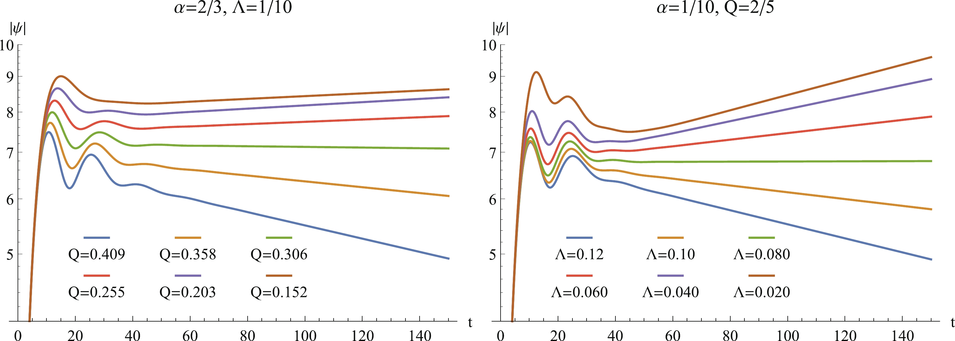

Figure 5

Figure 5.  (color online) Left panel: the time evolution of $|\psi(r_* = 88.4216,t)|$ at $\alpha = 2/3,\,\Lambda = 1/10$, where the different curves correspond to the different values of Q. Right panel: the time evolution of $|\psi(r_* = 88.4216,t)|$ at $\alpha = 1/10,\,Q = 2/5$, where the different curves correspond to the different values of $\Lambda$. For both plots we set $a = 88.4216,\,b = 1/10$.

DownLoad: Full-Size Img PowerPoint

It is also important to verify the validity of the AIM with respect to the time evolution. There are comprehensive methods for extracting frequencies from the perturbations' time-domain profiles, such as the Prony method used in [69]. Here, we extract $\omega_{\rm I}$ by computing $\partial_t\ln(|\psi|)$ for later times and compare the results with those obtained using the AIM. This simple process only allows to extract the imaginary part of the dominant mode and may not be sufficiently accurate when QNMs are close to each other. However, it is sufficiently good for the purposes of our current analysis. We provide the comparison in Table 1 (see the last two columns), from which we can see that all of the time evolution results perfectly agree with those of the AIM.

Finally, we show the unstable region of the charged EGB-dS black hole under charged scalar perturbation in Fig. 6. The black hole is unstable only when $\Lambda$ and Q are not too large. As $\Lambda$ or Q increases, the black hole becomes less unstable. For positive $\alpha$, the unstable region shrinks. For negative $\alpha$, the unstable region widens. Although we do not show the results for $\Lambda\to0$ owing to the limitation of our numerical method, we can expect that there should be sudden drops, since we have found that there is no instability for the asymptotic flat charged EGB black holes under charged scalar perturbations [34]. This phenomenon was also disclosed for RN-dS black holes in [70].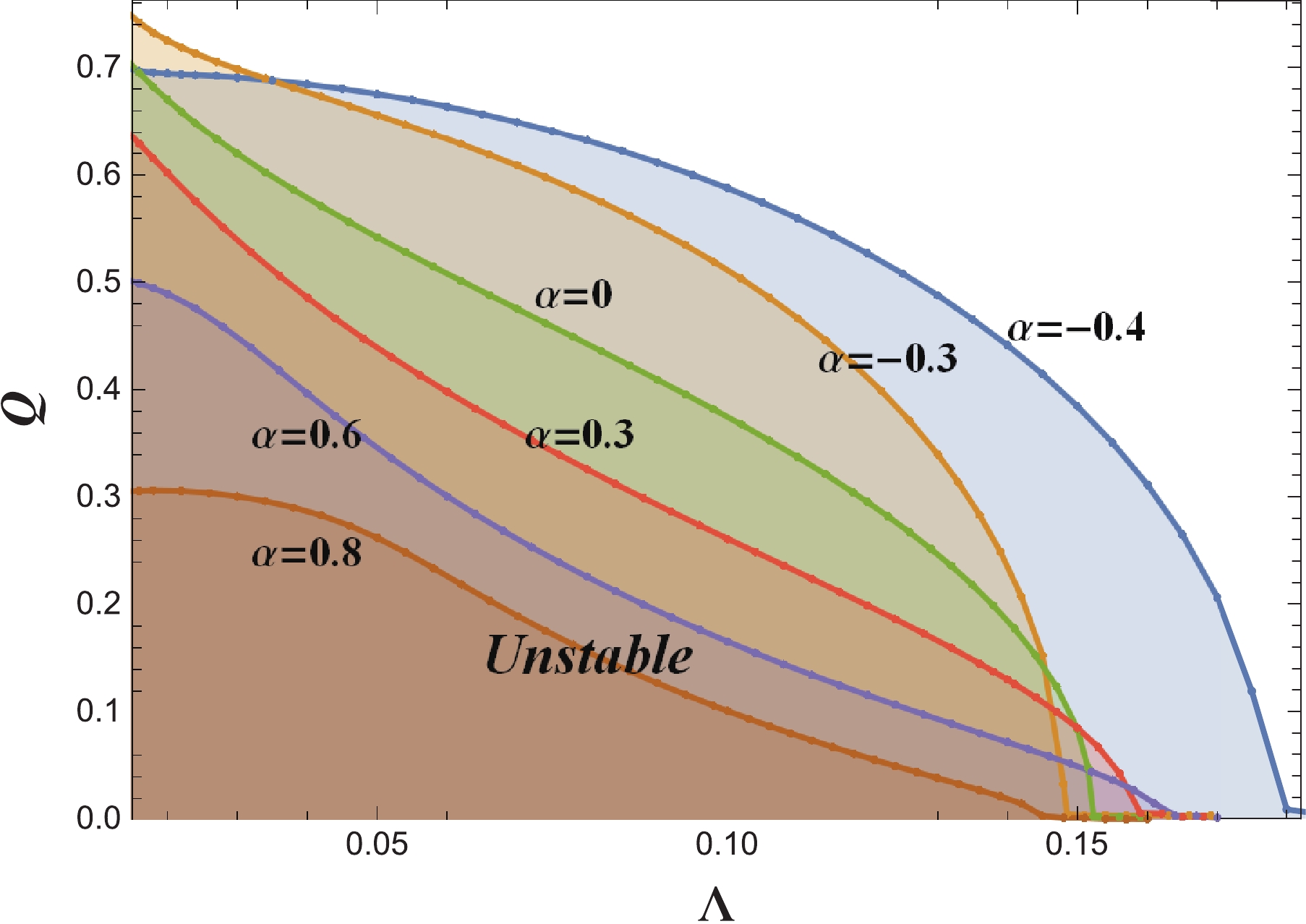

Figure 6

Figure 6.  (color online) The unstable region of the charged EGB-dS black hole under a charged scalar perturbation. The shadows under the constant $\alpha$ lines are the corresponding unstable regions. Here, $q = 1$.

DownLoad: Full-Size Img PowerPoint

D Effective potential

• I. INTRODUCTION
• II. THE 4D CHARGED EGB-DS BLACK HOLE
• III. THE CHARGED SCALAR PERTURBATION
• IV. THE INSTABILITY OF THE 4D CHARGED EGB-DS BLACK HOLE
•      A The asymptotic iteration method (AIM)
•      B The eigenfrequencies of the charged scalar perturbation
•      C Evolution of the perturbation field
•      D Effective potential
• V. SUMMARY AND DISCUSSION
• ACKNOWLEDGMENTS

Now let us take a look at the effective potential when $l = 0$. In the left panel of Fig. 7, we see that there is a negative potential well between $r_{+}$ and $r_{c}$. This potential well is the key point for the occurrence of instability. However, the negative effective potential does not guarantee $\omega_{\rm I}>0$. For example, the case $\alpha = 0.8$ has a negative potential well, but $\omega_{\rm I}<0$. Thus, the existence of a negative potential well can be viewed as the necessary but not sufficient condition for instability [78]. In the right panel of Fig. 7, the potential well disappears for larger $\alpha$. The perturbation wave can be easily absorbed by the black hole, and the corresponding background becomes stable with respect to charged scalar perturbations. Note that the positive cosmological constant is crucial here for creating the necessary potential well.

Figure 7

Figure 7.  (color online) The effective potential when $l = 0$. The left and right plots correspond to the orange lines in the upper right and lower right panels of Fig. 4, respectively.

DownLoad: Full-Size Img PowerPoint

Now, let us consider the eigenfrequencies of the charged scalar perturbation when $l = 1$. The fundamental modes are shown in Fig. 8. The left panel shows that the realtion $\omega_{\rm R}\propto Q$ still exists for higher l. However, $\alpha$ very weakly affects $\omega_{\rm R}$. All of the fundamental modes have $\omega_{\rm R} < \dfrac{qQ}{r_{c}}$ beyond the superradiant condition. The results in the left panel are different from those in Fig. 2. Here, $\omega_{\rm I}$ increases with Q and $\alpha$ monotonically. Note that all of the modes are stable now.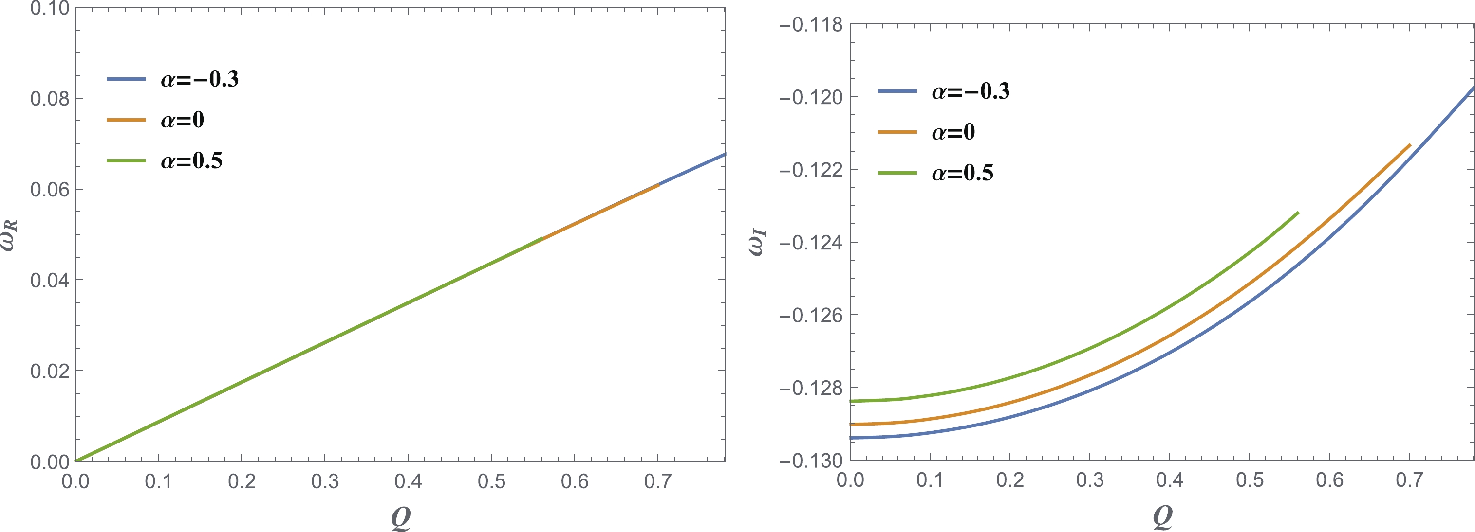

Figure 8

Figure 8.  (color online) The real part (left) and imaginary part (right) of the fundamental modes when $l = 1$. Here, $\Lambda = 0.05$. The results for other $\Lambda$ values are similar.

DownLoad: Full-Size Img PowerPoint

The stability for the higher l values can be explained using the effective potential, as shown in Fig. 9. There is only one potential barrier and there are no potential wells to accumulate the energy for triggering instability.

Figure 9

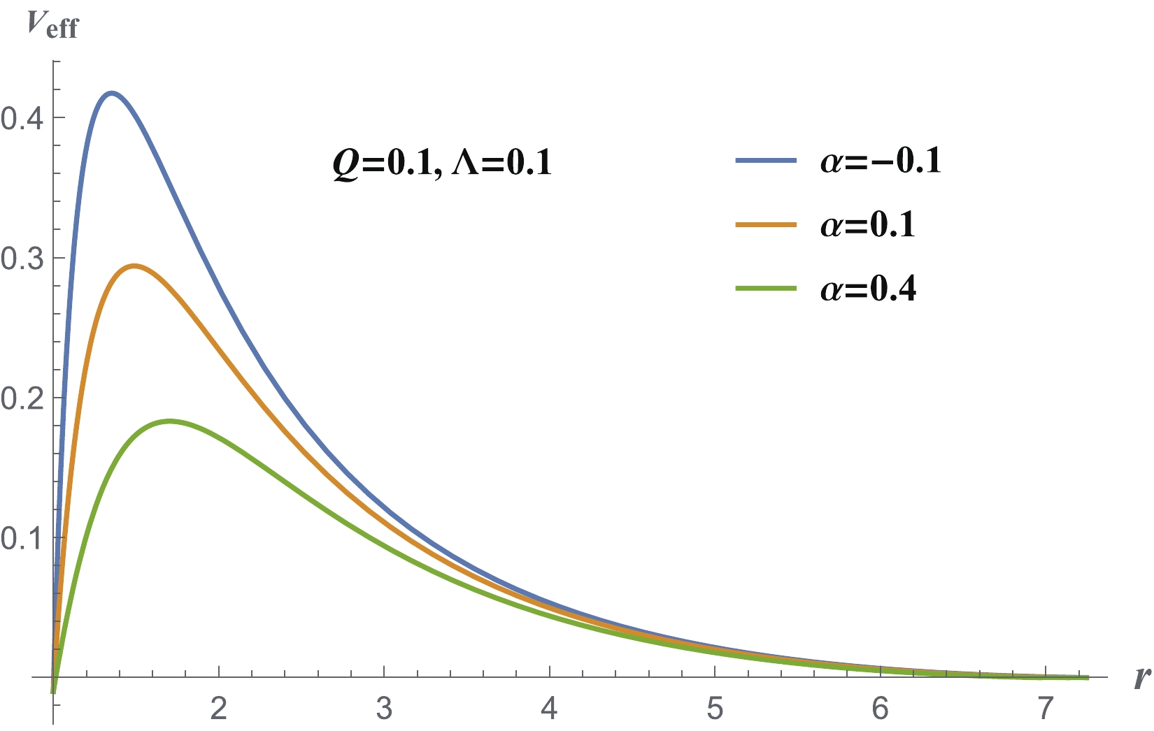
Figure 9.  (color online) The effective potential when $l = 1$. The results for other $Q,\;\Lambda$ values are similar.

DownLoad: Full-Size Img PowerPoint

A detailed time evolution for $l \neq 0$ is shown in Fig. 10. From these two panels, we see that the perturbations indeed decay in the long term, and larger l values yield a more significant decay of $\psi$; hence, no instability occurs for higher values of l.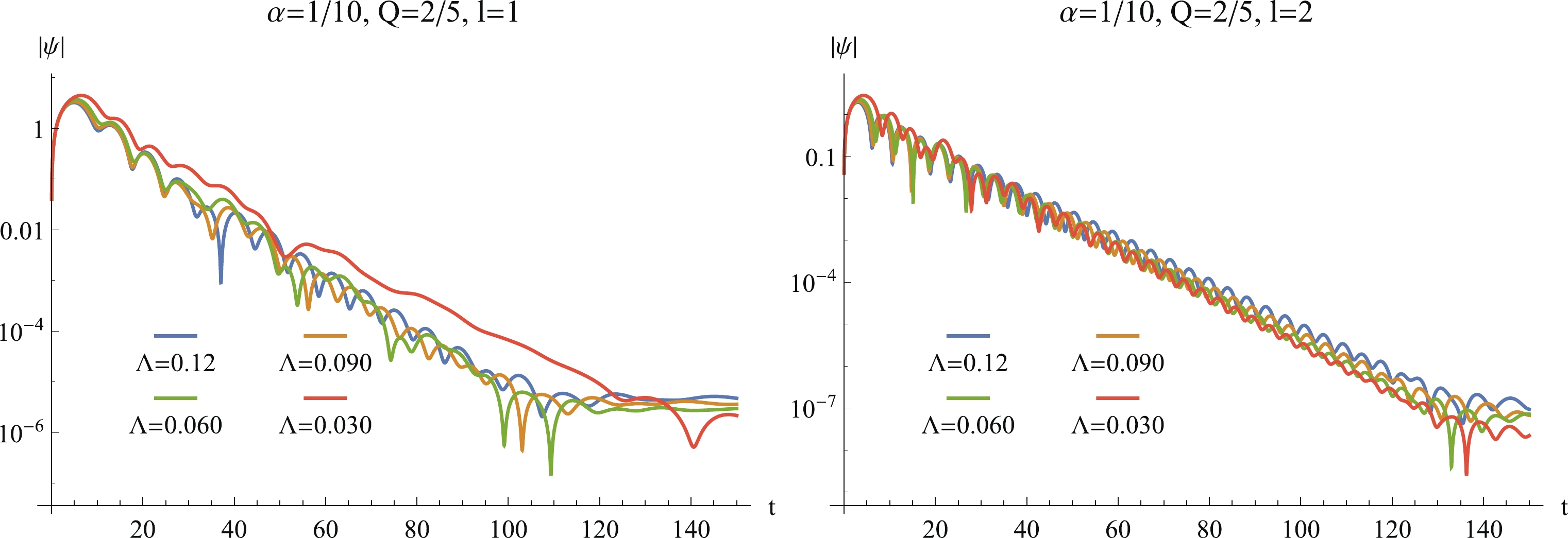

Figure 10

Figure 10.  (color online) The time evolution of $|\psi(r_* = 88.4216,t)|$ in the log plot at $\alpha = 1/10, \, Q = 2/5 ,\, a = 88.4216, \, b = 1/10$, and $q = 1$, where the different curves in both panels correspond to the different values of $\Lambda$. The left and the right panels show the results for $l = 1$ and $l = 2$, respectively.

DownLoad: Full-Size Img PowerPoint

V. SUMMARY AND DISCUSSION

• I. INTRODUCTION
• II. THE 4D CHARGED EGB-DS BLACK HOLE
• III. THE CHARGED SCALAR PERTURBATION
• IV. THE INSTABILITY OF THE 4D CHARGED EGB-DS BLACK HOLE
•      A The asymptotic iteration method (AIM)
•      B The eigenfrequencies of the charged scalar perturbation
•      C Evolution of the perturbation field
•      D Effective potential
• V. SUMMARY AND DISCUSSION
• ACKNOWLEDGMENTS

We studied the instability of charged 4D EGB-dS black holes with respect to charged massless scalar perturbations. This instability satisfies the superradiant condition. However, not all of the modes satisfying the superradiant condition are unstable. The precise mechanism of this instability is not well understood. Nevertheless, the positive cosmological constant $\Lambda$ should play a crucial role. The instability occurs when the cosmological constant is small. This is reminiscent of the Gregory-Laflamme instability [79] since there exists a hierarchy between the black hole event horizon and the cosmological horizon. The instability here is different from the "$\Lambda$ instability" found in [35, 64-68], which occurs when the black hole charge and the cosmological constant are large.

We analyzed this instability from the viewpoint of the effective potential. Higher l has only one potential barrier beyond the event horizon. The perturbation dissipates and does not lead to instability. The monopole $l = 0$ has a negative potential well between the event horizon and cosmological horizon, which can accumulate the energy necessary fortriggering the instability. But the negative potential well is just the necessary but not sufficient condition for the instability.

Unlike the case of the asymptotic flat spacetime, the effect of the GB coupling constant $\alpha$ on the perturbation is relevant to the black hole charge and cosmological constant. It makes an unstable black hole more unstable when both the black hole charge and cosmological constant are small and makes a stable black hole more stable when the black hole charge is large. Weakly charged black holes in the dS spacetime are always unstable. The existence of $\alpha$ does not change this phenomenon qualitatively. However, $\alpha$ can change the qualitative behavior when the black hole charge is large and make unstable black holes stable. We show that the unstable region of ($\Lambda,Q$) shrinks for positive $\alpha$ and enlarges for negative $\alpha$. Unfortunately, our results are not sufficiently accurate for $\Lambda \to 0$, owing to the limitation of our numerical method. The case in which a black hole becomes extremal is also beyond the scope of this method. Stability of extremal black holes may be very different from that of non-extremal black holes. There is a universal "horizon instability" [80-82]. We leave these issues to further studies.

We point out several topics worthy of further investigations. Stability with respect to massive perturbations should be explored in detail to reveal how the mass term affects stability with respect to charged perturbations. The stability of the 4D charged Einstein-Gauss-Bonnet anti de-Sitter black hole would be a very interesting issue to address as well. We plan to explore these questions in the near future.

ACKNOWLEDGMENTS

• I. INTRODUCTION
• II. THE 4D CHARGED EGB-DS BLACK HOLE
• III. THE CHARGED SCALAR PERTURBATION
• IV. THE INSTABILITY OF THE 4D CHARGED EGB-DS BLACK HOLE
•      A The asymptotic iteration method (AIM)
•      B The eigenfrequencies of the charged scalar perturbation
•      C Evolution of the perturbation field
•      D Effective potential
• V. SUMMARY AND DISCUSSION
• ACKNOWLEDGMENTS

We thank Peng-Cheng Li, Minyong Guo, and Shao-Jun Zhang for helpful discussions. Peng Liu would like to thank Yun-Ha Zha for her kind encouragement during this work.

References