


 Abstract
 HTML
HTML Reference
 Related
 PDF
PDF


-
Lorentz invariance (LI) is the most fundamental principle of general relativity (GR) and the standard model (SM) in particle physics. It is, therefore, not surprising that most theories of gravity encompass this symmetry, and little attention has been paid to understanding the implications of the breaking of LI. However, LI should not be an exact principle for all energy scales [1]. For example, when one considers the unification of quantum mechanics and GR, it should not be applicable. Both GR and the SM are based on LI and the spacetime background, but they address problems in profoundly different ways. GR is a classical field theory in curved spacetime that ignores all the quantum features of particles, whereas the SM is a quantum field theory in flat spacetime that disregards the gravitational effects of particles. For collisions of particles with energies on the order of
$ 10^{30} $ eV (above the Planck scale), the gravitational interactions estimated by GR are very powerful, and gravity should not be ignored [2]. Thus, on this scale of very high energies, one has to reconsider combining the SM with GR in a unified theory, i.e., "quantum gravity". Therefore, studying the Lorentz violation (LV) is a useful approach toward investigating the foundations of modern physics. This involves studying the LV in the neutrino range [3], the standard-model extension (SME) [4], the LV in the non-gravity range [5], and the LV effects on the creation of atmospheric showers [6].Experimental confirmation of this idea of quantum gravity is challenging because direct experiments on the Planck scale are impractical. However, suppressed effects, emerging from the underlying unified quantum gravity theory, might be observable on our low energy scale. Thus, the search for reminiscent quantum gravity effects in the low energy regime has attracted significant attention over the last decades. The combination of GR and the SM provides a remarkably successful description of nature. The SME is an effective field theory that studies gravity and the SM on low energy scales. It couples the SM to GR, enabling dynamical curvature modes, and involves extra items embracing information about the LV happening on the Planck scale [7]. The LV items in the SME have the form of Lorentz-violating operators coupled to coefficients with Lorentz indices. The appearance of the LV in a local Lorentz frame is manifested by a nonzero vacuum value for one or more quantities taking along local Lorentz indices. A specific theory is the "bumblebee" pattern, where the LV arises owing to the dynamics of a single vector or axial-vector field
$ B_\mu $ , known as the bumblebee field. This model is a simple effective theory of gravity with the LV in the SME and a subset of the Einstein-aether theory [8-10]. It is controlled by a potential revealing a minimum scrolls to its vacuum expectation value, showing that the vacuum of the theory obtains a preferential direction in the spacetime. The bumblebee gravitational model was first studied by Kostelecky and Samuel in 1989 [11, 12] as a specific pattern for an unprompted LV.Deriving black hole solutions is a very requisite task in any theory of gravity, because these solutions yield a large amount of information about quantum gravity. In 2018, R. Casana et al. gave an exact Schwarzschild-like solution in this bumblebee gravity model and considered some classical tests for it [13]. Then, Rong-Jia Yang et al. considered the accretion onto this black hole [14] and discovered that LV parameter
$ \ell $ decreases the mass accretion rate. The rotating black hole solutions are the most relational subsets for astrophysics. In 2020, C. Ding et al. found an exact Kerr-like solution by solving Einstein-bumblebee gravitational field equations and studied its black hole shadow [15]. However, this solution does not seem to meet the bumblebee field motion equation requirements. Thus, in the present paper, we seek a slowly rotating black hole solution for both of the following cases:$ b_\mu = (0,b(r), 0,0) $ and$ b_\mu = (0,b(r),\mathfrak{b}(\theta),0) $ .Then, we study the black hole greybody factor and obtain some deviations from GR and some LV gravity theories. The remainder of the paper is organized as follows. In Sec. II, we provide the necessary background on the Einstein-bumblebee theory. In Sec. III, we derive the slowly rotating black hole solution by solving the gravitational field equations. In Sec. IV, we study the black hole greybody factor and report some effects of Lorentz breaking constant
$ \ell $ . Sec. V contains the summary of our work. -
In the bumblebee gravity theory, bumblebee vector field
$ B_{\mu} $ attains a nonzero vacuum expectation value via a given potential, leading to a spontaneous Lorentz symmetry breaking in the gravitational sector. Its action [16] is$ \begin{aligned}[b] {\cal{S}} =& \int {\rm d}^4x\sqrt{-g}\Biggr[\frac{1}{16\pi G_N}({\cal{R}}-2\Lambda+\varrho B^{\mu}B^{\nu}{\cal{R}}_{\mu\nu}\\ &+\sigma B_\mu B^\mu {\cal{R}})-\frac{\tau_1}{4}B^{\mu\nu}B_{\mu\nu}+\frac{\tau_2}{2}D_\mu B_\nu D^\mu B^\nu \\ &+\frac{\tau_3}{2}D_\mu B^\mu D_\nu B^\nu-V(B_\mu B^{\mu}\mp b^2)+{\cal{L}}_M\Biggr], \end{aligned} $

(1) where
$ b^2 $ is a real positive constant. The Lorentz and/or$ {\rm CPT} $ (charge conjugation, parity, and time reversal) violation is opened by potential$ V(B_\mu B^{\,\mu}\mp b^2) $ . It yields a nonzero vacuum expectation value (VEV) for bumblebee field$ B_{\,\mu} $ , implying that the vacuum in this theory gets a preferential direction in the spacetime. This potential is assumed to have a minimum at$ B^{\,\mu}B_{\mu}\pm b^2 = 0 $ and$ V'(b_{\mu}b^{\mu}) = 0 $ to assure the breaking of the$ U(1) $ symmetry, where field$ B_{\mu} $ obtains a nonzero VEV,$ \langle B^{\,\mu}\rangle = b^{\mu} $ . Vector$ b^{\mu} $ is a function of the spacetime coordinates and has a constant value of$ b_{\mu}b^{\mu} = \mp b^2 $ , where the$ \pm $ signs imply that$ b^{\mu} $ is timelike or spacelike, respectively. The bumblebee field strength is$ B_{\mu\nu} = \partial_{\mu}B_{\nu}-\partial_{\nu}B_{\mu}. $

(2) Real constants
$ \varrho,\;\sigma,\;\tau_1,\;\tau_2,\;\tau_3 $ determine the form of the kinetic terms for the bumblebee field. Term$ {\cal{L}}_M $ represents possible interactions with matter or external currents. Note that if$ \varrho = \sigma = 0 $ and with a linear Lagrange-multiplier potential$ V = \lambda (B_\mu B^{\mu}\mp b^2), $

(3) this bumblebee model becomes a special case of the Einstein-aether theory [16]. In the Einstein-aether theory [9, 10], the Lorentz symmetry is broken by an introduced tensor field,
$ u^a $ , with the constraint$ u_au^a = -1 $ , termed aether, which is timelike everywhere and at all times. Then, a preferred time direction exists at every point of the spacetime, i.e., a preferred frame of reference. The introduction of the aether vector allows for some novel effects, e.g., matter fields can travel faster than the speed of light, which has been dubbed superluminal particles. In Ref. [9], we derived a series of charged Einstein-aether black hole solutions in 4 dimensional spacetime and studied their Smarr formula. In Ref. [10], we obtained a series of neutral and charged black hole solutions in 3 dimensional spacetime.In this study, constant
$ \tau_1 = 1 $ ,$ \Lambda = \sigma = \tau_2 = \tau_3 = 0 $ , and there is no$ {\cal{L}}_M $ ; hence,$ \begin{aligned}[b] {\cal{S}} =& \int {\rm d}^4x\sqrt{-g}\Biggr[\frac{1}{16\pi G_N}({\cal{R}}+\varrho B^{\mu}B^{\nu}{\cal{R}}_{\mu\nu})\\ &-\frac{1}{4}B^{\mu\nu}B_{\mu\nu} -V(B_\mu B^{\mu}\mp b^2)\Biggr], \end{aligned}$

(4) where
$ \varrho $ dominates the non-minimal gravity interaction with bumblebee field$ B_\mu $ . Action (4) yields the gravitational field equation in vacuum,$ {\cal{R}}_{\mu\nu}-\frac{1}{2}g_{\mu\nu}{\cal{R}} = \kappa T_{\mu\nu}^B, $

(5) where
$ \kappa = 8\pi G_N $ , and the bumblebee energy momentum tensor,$ T_{\mu\nu}^B $ , is$ \begin{aligned}[b] T_{\mu\nu}^B =& B_{\mu\alpha}B^{\alpha}_{\;\nu}-\frac{1}{4}g_{\mu\nu} B^{\alpha\beta}B_{\alpha\beta}- g_{\mu\nu}V+ 2B_{\mu}B_{\nu}V'\\ &+\frac{\varrho}{\kappa}\Biggr[\frac{1}{2}g_{\mu\nu}B^{\alpha}B^{\beta}R_{\alpha\beta} -B_{\mu}B^{\alpha}R_{\alpha\nu}-B_{\nu}B^{\alpha}R_{\alpha\mu}\\ &+\frac{1}{2}\nabla_{\alpha}\nabla_{\mu}(B^{\alpha}B_{\nu}) +\frac{1}{2}\nabla_{\alpha}\nabla_{\nu}(B^{\alpha}B_{\mu}) \\ &-\frac{1}{2}\nabla^2(B^{\mu}B_{\nu})-\frac{1}{2} g_{\mu\nu}\nabla_{\alpha}\nabla_{\beta}(B^{\alpha}B^{\beta})\Biggr]. \end{aligned} $

(6) The prime denotes differentiation with respect to the argument,
$ V' = \frac{\partial V(x)}{\partial x}\Big|_{x = B^{\mu}B_{\mu}\pm b^2}. $

(7) Using the trace of Eq. (5), we obtain the trace-reversed version
$ \begin{aligned}[b] {\cal{R}}_{\mu\nu} =& \kappa T_{\mu\nu}^B+2\kappa g_{\mu\nu}V -\kappa g_{\mu\nu} B^{\alpha}B_{\alpha}V'+\frac{\varrho}{4}g_{\mu\nu}\nabla^2(B^{\alpha}B_{\alpha}) \\ &+\frac{\varrho}{2}g_{\mu\nu}\nabla_{\alpha}\nabla_{\beta}(B^{\alpha}B^{\beta}). \end{aligned} $

(8) The equation of motion for the bumblebee field is
$ \nabla ^{\mu}B_{\mu\nu} = 2V'B_\nu-\frac{\varrho}{\kappa}B^{\mu}R_{\mu\nu}. $

(9) In the following, we suppose that the bumblebee field is frosted at its VEV, i.e., it is
$ B_\mu = b_\mu, $

(10) then, the specific form of the potential controlling its dynamics is irrelevant. As a result, we have
$ V = 0,\; V' = 0 $ . Then, the first two terms in Eq. (6) are like those of the electromagnetic field; the only distinctions are the coupling terms to the Ricci tensor. Under this condition, Eq. (8) leads to the following gravitational field equations:$ \bar R_{\mu\nu} = 0, $

(11) with
$ \begin{aligned}[b] \bar R_{\mu\nu} =& {\cal{R}}_{\mu\nu}-\kappa b_{\mu\alpha}b^{\alpha}_{\;\nu}+\frac{\kappa}{4}g_{\mu\nu} b^{\alpha\beta}b_{\alpha\beta}+\varrho b_{\mu}b^{\alpha}{\cal{R}}_{\alpha\nu} \\ &+\varrho b_{\nu}b^{\alpha}{\cal{R}}_{\alpha\mu} -\frac{\varrho}{2}g_{\mu\nu}b^{\alpha}b^{\beta}{\cal{R}}_{\alpha\beta}+\bar B_{\mu\nu},\\ \bar B_{\mu\nu} =& -\frac{\varrho}{2}\Big[ \nabla_{\alpha}\nabla_{\mu}(b^{\alpha}b_{\nu}) +\nabla_{\alpha}\nabla_{\nu}(b^{\alpha}b_{\mu}) -\nabla^2(b_{\mu}b_{\nu})\Big]. \end{aligned}$

(12) In the next section, we derive the slowly rotating black hole solution by solving the gravitational equations in this Einstein-bumblebee model.
-
In this section, we derive the slowly rotating black hole solution by solving the Einstein-bumblebee gravitational equations. Rotating black hole solutions are of extreme importance in astrophysics. However, deriving an exact rotating solution is very troublesome. For example, the Schwarzschild black hole solution was obtained in 1916, soon after GR was presented [17]. However,only 47 years later, in 1963, its rotating counterpart was obtained [18]. Many scholars have used the Newman-Janis algorithm [19] to obtain a full① rotating black hole solution, but they have not checked the gravitational field equations with this obtained solution. Some authors have demonstrated that this method does not work for nonlinear sources [20].
In Ref. [15], we have found an exact Kerr-like solution for bumblebee field
$ b_\mu = (0,b(r,\theta),0,0) $ by solving the gravitational field equations. However, this full rotating solution does not seem to meet the requirements of the bumblebee field equation. Considering only the case of$ b_\mu = (0,b(r),\mathfrak{b}(\theta),0) $ is very difficult, and it seems impractical to use the same method. Thus, here, we derive the slowly rotating black hole solution. The slowly rotating stationary axially symmetric black hole metric has the general form$ \begin{aligned}[b] {\rm d}s^2 =& -U(r){\rm d}t^2+\frac{1+\ell}{U(r)}{\rm d}r^2+2F(r)H(\theta)a{\rm d}t{\rm d}\phi\\ &+r^2{\rm d}\theta^2 +r^2\sin^2\theta {\rm d}\phi^2+{\cal{O}}(a^2), \end{aligned} $

(13) where a is a small constant denoting the rotating angular momentum, and
$ {\cal{O}}(a^2) $ denotes a small quantity, as small as or smaller than the second order of a, which can be ignored here. We will use this metric ansatz to set up the gravitational field equations.In this study, we assume that the bumblebee field acquires a radial vacuum energy expectation, since the spacetime curvature has a strong radial variation compared with very slow temporal changes. Thus, the bumblebee field is spacelike (
$ b_\mu b^\mu = $ positive constant) and is assumed to be$ \begin{aligned}[b] {\rm{Case \;A:}}\;b_\mu =& \big(0,b(r),0,0\big);\\ {\rm{Case \;B:}}\;b_\mu =& \big(0,b(r),\mathfrak{b}(\theta),0\big). \end{aligned} $

(14) Case A was considered by Casana and Ding et al. in Ref. [13, 15] for the bumblebee field coupled to the gravitational field. Case B was considered by Chen et al. in Ref. [21] for the bumblebee field coupled to the electromagnetic field. Then, the bumblebee field strength is
$ b_{\mu\nu} = \partial_{\mu}b_{\nu}-\partial_{\nu}b_{\mu}, $

(15) whose components are all zero for cases A and B. Their divergences are all zero as well, i.e.,
$ \nabla^{\mu}b_{\mu\nu} = 0. $

(16) From the equation of motion (9), we have
$ b^{\mu}{\cal{R}}_{\mu\nu} = 0 . $

(17) Gravitational field equation (11) becomes
$ {\cal{R}}_{\mu\nu}+\bar B_{\mu\nu} = 0. $

(18) The explicit form of
$ b_\mu $ is$ \begin{aligned}[b] {\rm{Case \;A:}}\;b_\mu =& \left(0,b_0\sqrt{\frac{1+\ell}{U(r)}},0,0\right);\\ {\rm{Case \;B:}}\;b_\mu =& \left(0,b_0\sqrt{\frac{1+\ell}{U(r)}}\;,ab_0\cos\theta,0\right), \end{aligned}$

(19) where
$ b_0 $ is a real constant. The amplitude of this bumblebee field is$ b_\mu b^{\mu} = g^{\mu\nu}b_\mu b_{\nu} = b_0^2, $

(20) for case A; for case B, it is
$ b_\mu b^{\mu} = g^{\mu\nu}b_\mu b_{\nu} = b_0^2+{\cal{O}}(a^2), $

(21) which are both consistent with the condition of
$ b_\mu b^\mu = $ positive constant.For metric (13), the nonzero components of the Ricci tensor are
$ {\cal{R}}_{tt},\;{\cal{R}}_{t\phi},\;{\cal{R}}_{rr}, \;{\cal{R}}_{r\theta},\;{\cal{R}}_{\theta\theta},\;{\cal{R}}_{\phi\phi} $ , shown in the appendix. We consider the following gravitational field equations (for both cases A and B):$ {\cal{R}}_{rr}+\bar B_{rr} = -\frac{1}{2rU}(rU''+2U')+{\cal{O}}(a^2) = 0, $

(22) $ \begin{aligned}[b] {\cal{R}}_{t\phi}+\bar B_{t\phi} =& -\frac{a}{2}\Biggr(HUF''+2FH\frac{U'}{r}\\ &+\frac{F}{r^2}H'' -\frac{F\cos\theta}{r^2\sin\theta}H'\Biggr)+{\cal{O}}(a^2) = 0, \end{aligned} $

(23) where the prime
$ ' $ is the derivative with respect to the corresponding argument. From Eq. (22), we obtain function$ U(r) $ ; then,$ U = -\frac{C_1}{r}+C_2, $

(24) where
$ C_1,\;C_2 $ are constants. Using the asymptotic flatness condition, we set$ C_2 = 1 $ and$ C_1 = 2M $ , where M is the mass of the black hole; then,$ U = 1-\frac{2M}{r}. $

(25) From Eq. (23), we obtain functions
$ F(r) $ and$ H(\theta) $ ; then,$ F = \frac{2M}{r}, \;\;\;\;H = \sin^2\theta. $

(26) Lastly, substituting these quantities into Eqns. (13) and (19), we obtain bumblebee field
$b_\mu = (0, \;b_0 $ $ \sqrt{(1+\ell)r/(r-2M)},\;0,\;0) $ for case A and$ b_\mu = (0,\;b_0 $ $\sqrt{(1+\ell)r/(r-2M)},\;ab_0\cos\theta,\;0)$ for case B. The slowly rotating metric in the bumblebee gravity in both cases is$ \begin{aligned}[b] {\rm d}s^2 =& - \left(1-\frac{2M}{r}\right){\rm d}t^2-\frac{4Ma\sin^2\theta}{r} {\rm d}t{\rm d}\varphi\\ &+\frac{(1+\ell)r}{r-2M}{\rm d}r^2+r^2{\rm d}\theta^2 +r^2\sin^2\theta {\rm d}\phi^2. \end{aligned}$

(27) If
$ \ell\rightarrow0 $ , it recovers the usual slowly rotating Kerr metric. When$ a\rightarrow0 $ , it becomes$ {\rm d}s^2 = - \left(1-\frac{2M}{r}\right){\rm d}t^2+\frac{1+\ell}{1-2M/r}{\rm d}r^2+r^2{\rm d}\theta^2 +r^2\sin^2\theta {\rm d}\varphi^2, $

(28) which is the same as that in Ref. [13]. Metric (27) represents a Lorentz-violating black hole solution with slowly rotating angular momentum a. It is easy to see that the horizon is located at
$ r_+ = 2M $ .Next, we consider the bumblebee motion equation and check for other gravitational equations. From bumblebee field motion equation (17), we obtain the following equation:
$ b^r{\cal{R}}_{rr}+b^\theta{\cal{R}}_{\theta r} = 0,\;\;\;\; b^r{\cal{R}}_{r\theta}+b^\theta{\cal{R}}_{\theta \theta} = 0. $

(29) From the appendix, we have
${\cal{R}}_{rr} = -(rU''+2U')/2rU+ $ ${\cal{O}}(a^2) = 0+{\cal{O}}(a^2)$ ,$ {\cal{R}}_{r\theta} = 0+{\cal{O}}(a^2) $ , and${\cal{R}}_{\theta \theta} = -(rU'+U)/ (1+\ell)+1+{\cal{O}}(a^2) = \ell/(1+\ell)+{\cal{O}}(a^2)$ . We can observe that the first equation is fulfilled for both cases; the second one can be fulfilled for case A (because$ b^\theta = 0 $ ). However, the second equation for case B is$ b^\theta{\cal{R}}_{\theta \theta} = \frac{b_0\cos\theta}{1+\ell}\cdot\frac{a\ell}{r^2}+{\cal{O}}(a^2). $

(30) If and only if coupling constant
$ \ell $ is also sufficiently smaller than angular momentum a, the second motion equation can be fulfilled for case B. As for the other gravitational equations, for case A, they are,$ {\cal{R}}_{tt}+\bar B_{tt} = 0 +{\cal{O}}(a^2), $

(31) $ {\cal{R}}_{r\theta}+\bar B_{r\theta} = 0+{\cal{O}}(a^2), $

(32) $ {\cal{R}}_{\theta\theta}+\bar B_{\theta\theta} = 0+{\cal{O}}(a^2), $

(33) $ {\cal{R}}_{\phi\phi}+\bar B_{\phi\phi} = 0+{\cal{O}}(a^2), $

(34) which are all fulfilled. However, for case B, there are similar limits for these equations to be fulfilled, i.e.,
$ {\cal{R}}_{tt}+\bar B_{tt} = \frac{\cos2\theta}{2\sqrt{1+\ell}\sin\theta}\cdot\frac{a\ell\sqrt{U}}{r^2} +{\cal{O}}(a^2), $

(35) $ {\cal{R}}_{r\theta}+\bar B_{r\theta} = \frac{\cos\theta}{\sqrt{1+\ell}}\cdot\frac{a\ell}{r^2\sqrt{U}}+{\cal{O}}(a^2), $

(36) $ \begin{aligned}[b]{\cal{R}}_{\theta\theta}+\bar B_{\theta\theta} = &\frac{1}{\sqrt{1+\ell}\sin\theta}\cdot\frac{a\ell}{r\sqrt{U}} (r\sin^2\theta U'\\ &-\cos2\theta U)+{\cal{O}}(a^2), \end{aligned} $

(37) $ \begin{aligned}[b]{\cal{R}}_{\phi\phi}+\bar B_{\phi\phi} =& \frac{\sin\theta}{2\sqrt{1+\ell}}\cdot\frac{a\ell}{r\sqrt{U}} (r\cos^2\theta U'\\ &+2\cos2\theta U)+{\cal{O}}(a^2).\end{aligned} $

(38) In conclusion, there exists a slowly rotating black hole solution for case A, for an arbitrary coupling constant
$ \ell $ ; however, for case B, there exists a slowly rotating black hole solution if and only if the coupling constant is sufficiently smaller than rotating angular momentum a. It is interesting that in both cases, the forms of the solutions are the same. Up to date, a full rotating black hole solution has not been derived. Thus, for case A, when the slow rotation restrictions on a are relaxed, we have$ b_\mu = (0,b(r,\theta),0,0) $ , and the obtained full rotating solution [15] does not seem to meet the bumblebee field equation requirements; for case B, it remains an open issue whether there exists a full rotating solution when coupling constant$ \ell $ is sufficiently small. Therefore, one cannot use the Newman-Janis algorithm to obtain a full rotating black hole solution. This is similar to the Einstein-aether theory, where only a slowly rotating black hole solution exists [22], with a spherically symmetric (hypersurface-orthogonal) aether field configuration for$ c_{14} = 0, c_{123}\neq0 $ [23]. -
The above slowly rotating solution contains the effects of the bumblebee field and can be used to study the effects of the bumblebee field on the black hole greybody factor. In this section, we study some observational signatures on the Lorentz-violating parameter,
$ \ell $ , by analyzing the black hole greybody factor (Hawking radiation) with metric (27) and try to find some deviations from GR and some similarities to other LV black holes.In Ref. [24], we obtained analytical expressions for the greybody factor and dynamic evolution for the scalar field in the Ho
$ \mathop {\rm{r}} \limits^ \smallsmile$ ava-Lifshitz black hole. In Ref. [25], we studied the greybody factor of the slowly rotating Kerr-Newman black hole in the non-minimal derivative coupling theory. In this model, the kinetic term of scalar field$ \psi $ is only coupled with the Einstein tensor,$ G^{\mu\nu}\partial_\mu\psi\partial_\nu\psi $ . The coupling was confirmed to be breaking the Lorentz symmetry [26].The Klein-Gordon equation in the Einstein-bumblebee black hole spacetime (the scalar field coupling to the bumblebee field is ignored here) is
$ \dfrac{1}{\sqrt{-g}}\partial_{\mu}\left(\sqrt{-g}g^{\mu\nu}\partial_{\nu}\psi\right) = 0. $

(39) Using spherical harmonics
$ \psi(t,r,\theta,\varphi) = {\rm e}^{-{\rm i}\omega t}\,{\rm e}^{{\rm i} m \varphi}\,R_{\omega lm}(r) \,T^{m}_{l}(\theta, a \omega)\,, $

(40) and substituting metric (27) into Eq. (39), we obtain the following radial equation:
$ \frac{\rm d}{{\rm d}r}\Bigg[(r^2-2Mr)\, \frac{{\rm d} R_{\omega l m}}{{\rm d}r}\Bigg]+ (1+\ell)\Bigg[\frac{r^2\omega(r^2\omega-2am)}{r^2-2Mr} -l(l+1)+2am\omega \Bigg]R_{\omega l m} = 0\,. $

(41) Before attempting to solve it analytically, we first analyze the profile of the effective potential that characterizes the emission process. Defining a new radial function,
$ R_{\omega l m}(r) = \frac{\tilde{R}_{\omega l m}(r)}{r}, $

(42) and using tortoise coordinate x as follows:
$ \frac{\rm d}{{\rm d}x} = \left(1-\frac{2M}{r}\right)\frac{\rm d}{{\rm d}r}, $

(43) Eq. (41) can be rewritten in the standard Schrödinger equation form as
$ \left(\frac{{\rm d}^2}{{\rm d}x^2}-V_{\rm eff}\right)\tilde{R}_{\omega l m}(x) = 0, $

(44) where the effective potential is
$\begin{aligned}[b] V_{\rm eff} =& (1+\ell)\left(-\omega^2+\frac{4M}{r^3}ma\omega\right)\\ &+\left(1-\frac{2M}{r}\right) \left[\frac{4M}{r^3}+(1+\ell)\frac{l(l+1)}{r^2}\right]. \end{aligned} $

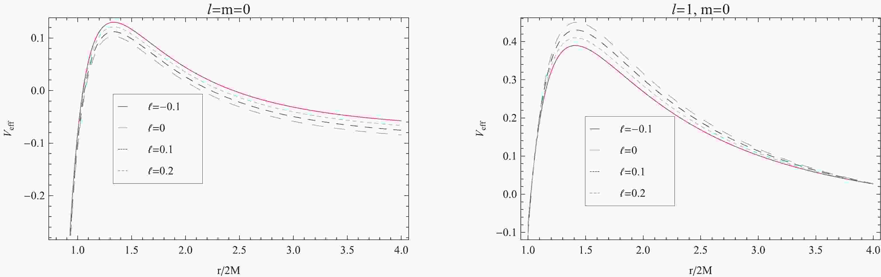
(45) For graphical analysis, we display the dependence of the effective potential on different parameters in Fig. 1. It is found that the gravitational barrier decreases gradually with the increase in LV coupling constant
$ \ell $ when$ l = 0 $ (left plot of Fig. 1), similar to the Einstein-aether theory [23] and non-minimal coupling theory [25]. However, the barrier increases with$ \ell $ when$ l = 1 $ (right plot of Fig. 1). Increasing the effective potential means reducing the emission of scalar fields; hence, LV coupling constant$ \ell $ affects the black hole greybody factor.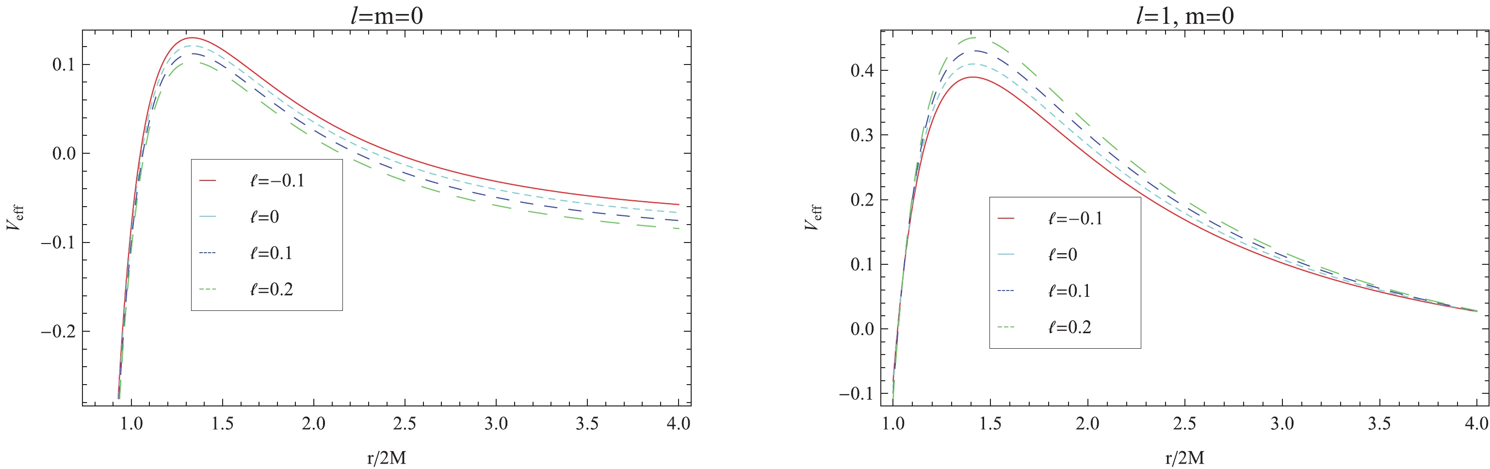
Figure 1. (color online) Variation of the potential,
$V_{\rm eff}$ , for different values of coupling constant$ \ell $ of a scalar field in the slowly rotating Einstein-bumblebee black hole, for fixed quantity$ \omega = 0.3 $ .Now, we derive the analytical solution of Eq. (41). We change radial variable r [24, 25] to function
$ f(r) $ as follows:$ r \rightarrow f(r) = 1-\frac{2M}{r} \,\,\Longrightarrow\, \frac{\rm d }{{\rm d}r} = \frac{1-f}{r}\frac{\rm d}{{\rm d}f}\,, $

(46) following which Eq. (41) becomes
$ f(1-f)\frac{{\rm d}^2R(f)}{{\rm d} f^2}+(1-f)\frac{{\rm d} R(f)}{{\rm d} f} +\bigg[\frac{K^2_*}{(1-f)f} -\frac{\Lambda^m_l}{(1-f)}\bigg]R(f) = 0, $

(47) where②
$\begin{aligned}[b] K_* =& \left(\omega r_+-a_*m\right)\sqrt{1+\ell},\;\\ a_* =& a/r_+,\; \Lambda^m_l = \sqrt{1+\ell}\big[l(l+1)-2ma\omega\big]. \end{aligned} $

(48) After using the redefinition,
$ R(f) = f^{\alpha}(1-f)^{\beta}F(f) $ , and constraints$ \alpha^2+K^2_* = 0,\;\;\;\;\beta^2-\beta+\big[K^2_* -\Lambda^m_l\big] = 0, $

(49) we observe that Eq. (47) is a hypergeometric equation,
$ f(1-f)\frac{{\rm d}^2F(f)}{{\rm d} f^2}+[c-(1+\tilde{a}+\tilde{b})f]\frac{{\rm {\rm d}} F(f)}{{\rm d} f}-\tilde{a}\tilde{b} F(f) = 0, $

(50) with
$ \tilde{a} = \alpha+\beta,\quad \tilde{b} = \alpha+\beta,\quad c = 1+2\alpha. $

(51) The above two constrains (49) show that parameters
$ \alpha $ and$ \beta $ are$ \alpha_{\pm} = \pm {\rm i}K_*, $

(52) $ \beta_{\pm} = \frac{1}{2}\bigg[1\pm\sqrt{1-4\big(K^2_* -\Lambda^m_l\big)} \;\bigg]. $

(53) Then, the exact analytical solution of Eq. (50) is
$\begin{aligned}[b] R(f) =& A_-f^{\alpha}(1-f)^{\beta}F(\tilde{a}, \tilde{b}, c; f)\\ &+A_+ f^{-\alpha}(1-f)^{\beta}F(\tilde{a}-c+1, \tilde{b}-c+1, 2-c; f), \end{aligned} $

(54) where
$ A_+,\; A_- $ are arbitrary constants.Near the horizon,
$ r\rightarrow r_+ $ and$ f\rightarrow0 $ ; the solution is$ R_{\rm NH}(f) = A_-f^{\alpha_\mp}+A_+f^{\alpha_\pm}. $

(55) The boundary condition near the horizon is that no outgoing mode exists; hence, we consider either
$ A_- = 0 $ or$ A_+ = 0 $ , corresponding to the choice for$ \alpha_\pm $ . Here, we set$ \alpha = \alpha_- $ and$ A_+ = 0 $ . The convergence of the hypergeometric function$ F(\tilde{a}, \tilde{b}, c; f) $ will determine the sign of$ \beta $ , i.e., here, Re$ (c-\tilde{a}-\tilde{b})>0 $ ; then, we set$ \beta = \beta_- $ [24, 25]. Therefore, the asymptotic solution near the horizon$ (r\sim r_+) $ is$ R_{\rm NH}(f) = A_-f^{\alpha}(1-f)^{\beta}F(\tilde{a}, b, c; f). $

(56) Now, we can smoothly extend the near horizon solution (56) to the intermediate zone. We consider the property of the hypergeometric function [27] and alter its argument in the near horizon solution, from f to
$ 1-f $ $ \begin{aligned}[b] R_{\rm NH}(f) =& A_-f^{\alpha}(1-f)^{\beta}\Biggr[\frac{\Gamma(c)\Gamma(c-\tilde{a}-\tilde{b})} {\Gamma(c-\tilde{a})\Gamma(c-\tilde{b})} F(\tilde{a}, \tilde{b}, \tilde{a}+\tilde{b}-c+1; 1-f)+(1-f)^{c-\tilde{a}-\tilde{b}}\frac{\Gamma(c)\Gamma(\tilde{a}+\tilde{b}-c)}{\Gamma(\tilde{a})\Gamma(\tilde{b})}\\&\times F(c-\tilde{a}, c-\tilde{b}, c-\tilde{a}-\tilde{b}+1; 1-f)\Biggr]. \end{aligned} $

(57) When
$ r\gg r_+ $ , function$ (1-f) $ is$ 1-f = \frac{2M}{r}, $

(58) and then, the near horizon solution (57) can be reduced to
$ R_{\rm NH}(r)\simeq C_1r^{-\beta}+C_2r^{\beta-1} , $

(59) with
$ C_1 = A_-(2M)^{\beta} \frac{\Gamma(c)\Gamma(c-\tilde{a}-\tilde{b})}{\Gamma(c-\tilde{a})\Gamma(c-\tilde{b})}, $

(60) $ C_2 = A_-(2M)^{1-\beta}\frac{\Gamma(c)\Gamma(\tilde{a}+\tilde{b}-c)}{\Gamma(\tilde{a})\Gamma(\tilde{b})}. $

(61) In the far field region, we expand the wave equation (41) as a power series in
$ 1/r $ and maintain only the leading terms$ \frac{{\rm d}^2R_{\rm FF}(r)}{{\rm d}r^2}+\frac{2}{r}\frac{{\rm d}R_{\rm FF}(r)}{{\rm d} r}+(1+\ell)\bigg[\omega^2-\frac{l(l+1)}{r^2}\bigg]R_{\rm FF}(r) = 0. $

(62) It is easy to see that this is the usual Bessel equation. Therefore, the solution of the radial master equation (41) in the far-field limit is
$ R_{\rm FF}(r) = \frac{1}{\sqrt{r}}\bigg[B_1J_{\nu}(\sqrt{1+\ell}\omega r)+B_2Y_{\nu} (\sqrt{1+\ell}\omega r)\bigg], $

(63) where
$ J_{\nu}(\omega\;r) $ and$ Y_{\nu}(\omega\;r) $ are the first and second kind Bessel functions, respectively;$ \nu = \sqrt{(1+\ell)l(1+l)+1/4} $ .$ B_1 $ and$ B_2 $ are the integration constants. Now, we take limit$ r\rightarrow 0 $ and extend the far-field solution (63) to the small values of the radial coordinate. Then, Eq. (63) becomes$ R_{\rm FF}(r)\simeq\frac{B_1\left(\dfrac{\sqrt{1+\ell}\omega r}{2}\right)^{\nu}}{\sqrt{r}\;\Gamma(\nu+1)} -\frac{B_2\Gamma(\nu)}{\pi \sqrt{r}\;\left(\dfrac{\sqrt{1+\ell}\omega r}{2}\right)^{\nu}}. $

(64) After applying the conditions of low-energy and low-angular momentum limits
$ (\omega r_+)^2\ll1 $ and$ (a/r_+)^2\ll1 $ , both power coefficients in Eq. (59) become, approximately,$ -\beta \simeq -\frac{1}{2}+\nu + {\cal O}(\omega^2,a^2,a\omega), $

(65) $ (\beta-1)\simeq -\frac{1}{2}-\nu+ {\cal O}(\omega^2,a^2,a\omega). $

(66) Up to this point, it is easy to see that both extensions (59) and (64) of the near horizon and the far field solutions can be simplified to power-law representations with the same power coefficients,
$ r^{-1/2+\nu} $ and$ r^{-1/2-\nu} $ . By comparing the corresponding coefficients between Eqns. (59) and (64), we obtain two connections between$ C_1,\;C_2 $ and$ B_1,\;B_2 $ . Eliminating$ A_- $ , we gain the ratio between coefficients$ B_1,\; B_2 $ $ \begin{aligned}[b] B\equiv\frac{B_1}{B_2} = &-\frac{1}{\pi}\bigg[\frac{1}{\sqrt{1+\ell}\omega M}\bigg]^{2\nu} \nu\Gamma^2(\nu) \\ &\times\;\frac{ \Gamma(c-\tilde{a}-\tilde{b})\Gamma(\tilde{a})\Gamma(\tilde{b})}{\Gamma(\tilde{a}+\tilde{b}-c)\Gamma(c-\tilde{a})\Gamma(c-\tilde{b})}. \end{aligned} $

(67) In asymptotic regime
$ r\rightarrow \infty $ , the far-field solution can be rewritten as$ \begin{aligned}[b] R_{\rm FF}(r)\simeq & \frac{B_1+{\rm i}B_2}{\sqrt{2\pi\;\sqrt{1+\ell}\;\omega} r}{\rm e}^{-{\rm i}\sqrt{1+\ell}\;\omega r}\\ &+ \frac{B_1-{\rm i}B_2}{\sqrt{2\pi\;\sqrt{1+\ell}\;\omega} r}{\rm e}^{{\rm i}\sqrt{1+\ell}\;\omega r} \end{aligned}$

(68) $ \;\;\;\qquad = A^{(\infty)}_{\rm in}\dfrac{{\rm e}^{-{\rm i}\sqrt{1+\ell}\;\omega r}}{r} +A^{(\infty)}_{\rm out}\dfrac{{\rm e}^{{\rm i}\sqrt{1+\ell}\;\omega r}}{r}. $

(69) The absorption probability can be obtained from
$ |{\cal{A}}_{l m}|^2 = 1-\left|\frac{A^{(\infty)}_{\rm out}}{A^{(\infty)}_{\rm in}}\right|^2 = 1-\left|\frac{B-i}{B+i}\right|^2 = \frac{2{\rm i}(B^*-B)}{BB^*+{\rm i} (B^*-B)+1}. $

(70) Substituting the expression for B from Eq. (67) into Eq. (70), we acquire some features of the absorption probability for the bumblebee field coupled with the Ricci tensor in the slowly rotating black hole spacetime in the low-energy limit.
In Fig. 2, we set the angular momentum to
$ a = 0.1 $ , and plot the absorption probability of a scalar particle for the first ($ l = 0 $ ) and second ($ l = 1 $ ) partial waves in the slowly rotating Einstein-bumblebee black hole spacetime. Evidently, the absorption probability,$ A_{l = 0} $ , rises with the increase in LV coupling constant$ \ell $ , which is analogous to the situation in the non-minimal coupling theory [25]. However,$ A_{l = 1} $ decreases with the increase in LV coupling constant$ \ell $ .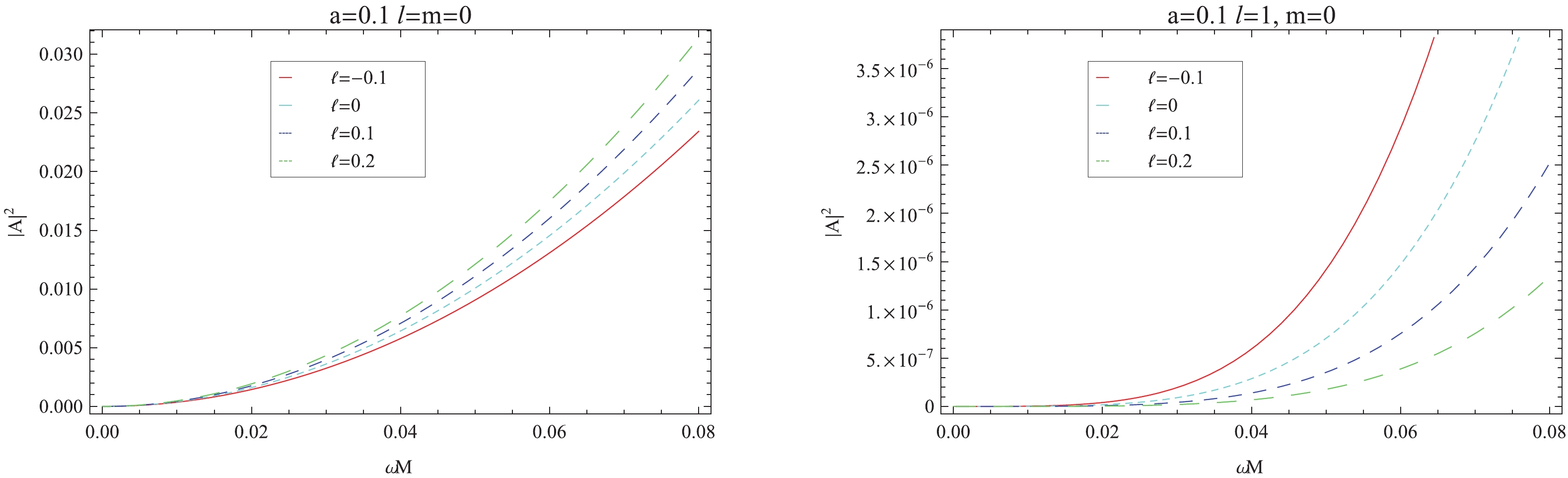
Figure 2. (color online) Variation of the absorption probability,
$ |A_{l m}|^2 $ , of a scalar field in the slowly rotating Einstein-bumblebee black hole, for a fixed angular momentum with$ a = 0.1 $ and$ m = 0 $ .In the case of
$ l\geqslant 1 $ , there is a superradiation region, where$ m = 1, 2, \cdots, l $ , which is analogous to [25]. In Fig. 3, we show the dependence of the absorption probability on angular indices l and m, for different$ \ell $ and a. From the above two graphics in Fig. 3, for the super-radiation case, angular momentum a improves the usual radiation ($ m = -1 $ ) and the super-radiation ($ m = 1 $ ) for weak coupling. We note the attenuation of$ |A_{\ell m}|^2 $ for$ l\geqslant 1 $ . This means that the first partial wave,$ l = 0 $ , leads the other ones with respect to the absorption probability. This is similar to the situation for a scalar field without any couplings.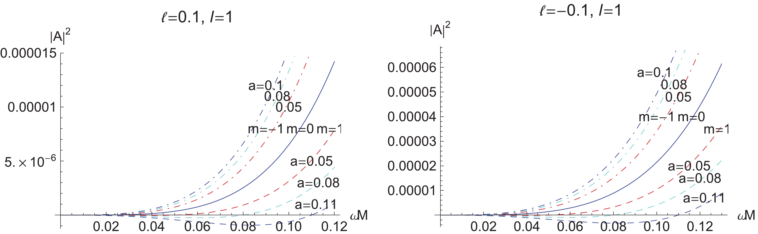
Figure 3. (color online) Dependence of absorption probability
$ |A_{l m}|^2 $ of a scalar field on angular momentum a in the slowly rotating Einstein-bumblebee black hole, for fixed$ \ell = 0.1,-0.1;l = 1 $ ; and$ m = 1,0,-1 $ . -
In this paper, we have studied the slowly rotating, asymptotically flat black hole solutions of the Einstein-bumblebee theory, for both cases of the bumblebee field:
$ b_\mu = (0,b(r),0,0) $ and$ b_\mu = (0,b(r),\mathfrak{b}(\theta),0) $ . In the case of the radial Lorentz symmetry breaking, we have obtained an exact slowly rotating black hole solution for the$ rr $ and$ t\phi $ components of the gravitational field equations. In the$ a\rightarrow0 $ limit of the angular momentum, the solution reduces to a Schwarzschild like solution [13]; in the$ \ell\rightarrow0 $ limit of the LV constant, we obtain a slowly rotating Kerr black hole solution. We also reported the horizon positions.With this solution, we then check the other gravitational equations and the bumblebee motion equations. In the case of bumblebee field
$ b_\mu = (0,b(r),0,0) $ , all of these equations can be fulfilled for an arbitrary coupling constant$ \ell $ . In the case of bumblebee field$ b_\mu = (0,b(r),\mathfrak{b}(\theta),0) $ , all of these equations can be fulfilled if and only if coupling constant$ \ell $ is as small as or smaller than slowly rotating angular momentum a. If LV coupling constant$ \ell $ is not small, the slowly rotating solution cannot exist. Thus far, no full rotating black hole solutions have been published; hence, the Newman-Janis algorithm cannot be used to obtain a rotating solution, because it may not satisfy the entire set of field equations. This is similar to the Einstein-aether theory, where there can only exist a slowly rotating black hole solution. The existence of a full rotating black hole solution for case B for very small values of the coupling constant remains an open issue.With this obtained black hole solution, we studied some LV effects on future astronomical events. In particular, we studied the black hole greybody factor for some observational effects of LV constant
$ \ell $ . We reported the deviation effects of the LV from GR (a slowly rotating Kerr black hole); for the angular momentum index of$ l = 0 $ , the effective potential,$ V_{\rm eff} $ , decreased with the increase in LV coupling constant$ \ell $ . These decreases were similar to those for the Einstein-aether black hole [23] and non-minimal derivative coupling theory [25], which are also LV black holes. The LV affected the greybody factor by increasing the absorption probability, similar to the non-minimal derivative coupling theory [25]. These differences can be detected by new generation gravitational antennas. -
The authors would like to thank Prof. Songbai Chen for useful suggestions.
-
In this appendix, we show the nonzero components of the Ricci tensor for metric (13). They are as follows:
$\tag{A1} {\cal{R}}_{tt} = \dfrac{U}{1+\ell}\left[\dfrac{U''}{2}+\dfrac{r\sin^2\theta UU'}{\Sigma}\right]+\dfrac{a^2}{2\Sigma}\left[\frac{F^2U}{r^2}H'^2 +\dfrac{H^2U^2}{1+\ell}U'^2+\dfrac{F^2H^2U}{(1+\ell)r}U'-\dfrac{FH^2U}{1+\ell}F'U'\right] , $

$ \tag{A2} {\cal{R}}_{t\phi} = -\frac{a}{2}\left[\frac{HUF''}{1+\ell}+\frac{FH''}{r^2} +\frac{rFHU\sin^2\theta}{(1+\ell)\Sigma}U'-\frac{FU\cos\theta\sin\theta}{\Sigma}H' \right]-\frac{a^3F^2H^3}{2\Sigma(1+\ell)}\left(\frac{1}{2}F'U' +\frac{U}{r}F'\right), $

$\tag{A3}\begin{aligned}[b] {\cal{R}}_{rr} =& -\frac{r^2\sin^2\theta}{\Sigma}\left(\frac{U''}{2} +\frac{r\sin^2\theta}{\Sigma}UU'\right)-\frac{a^2F^2H^2}{\Sigma}F''+\frac{a^2H^2}{\Sigma^2}\left[-\frac{1}{2}\bar\Sigma F'^2-\frac{F^2r^2\sin\theta}{4U}U'^2\right.\\ &\left.+\frac{F\bar\Sigma}{2U}F'U'+2rU\sin^2\theta FF'-\frac{F^2(5r^2U\sin^2\theta+a^2F^2H^2)}{2rU}U'-F^2U\sin^2\theta \right], \end{aligned}$

$ \tag{A4}\begin{aligned}[b] {\cal{R}}_{r\theta} =& \frac{a^2FH}{\Sigma^2} \Biggr[-\frac{1}{2}(a^2F^2H^2+3r^2U\sin^2\theta)F'H'+\frac{1}{2}Fr^2\sin\theta U'H'\\ &+\frac{F}{r}(a^2F^2H^2+2r^2U\sin^2\theta)H'+\frac{1}{2}HUr^2\sin2\theta F'-FHr\sin\theta\cos\theta (\frac{1}{2}rU'+U) \Biggr], \end{aligned} $

$\tag{A5}\begin{aligned}[b] {\cal{R}}_{\theta\theta} =& -\frac{r}{1+\ell}\left(U' +\frac{r^3U^3\sin^4\theta}{\Sigma^2}\right)+\frac{r^4U^2\sin^4\theta}{\Sigma^2}- \frac{a^2FH}{\Sigma}\Biggr[FH''-\frac{rFHU'}{2(1+\ell)} +\frac{HrU}{1+\ell}F'\Biggr]\\ &-\frac{a^2F^2}{\Sigma^2}\Biggr[\frac{1}{2}\bar\Sigma H'^2-HrU\sin2\theta H'+r^2H^2U\cos2\theta+\frac{r^2\sin^2\theta}{1+\ell}H^2U^2\Biggr], \end{aligned} $

$\tag{A6}\begin{aligned}[b] {\cal{R}}_{\phi\phi} =& -\frac{r^2U\sin^4\theta}{\Sigma}\left( \frac{rU'+U}{1+\ell}-1\right)+ \frac{a^2}{\Sigma}\Biggr[-\frac{1}{2}F^2\sin^2\theta H'^2+\frac{1}{2}F^2H\sin2\theta H'\\ &+ \frac{H^2\sin^2\theta}{1+\ell}\Biggr(-\frac{1}{2}Ur^2F'^2 +\frac{1}{2}F^2rU'+FUrF'-2F^2U\Biggr)-F^2H^2\cos2\theta\Biggr], \end{aligned} $

where
$ \Sigma $ and$ \bar\Sigma $ are$ \begin{aligned}[b] & \Sigma = r^2U\sin^2\theta+a^2F^2H^2,\\& \bar\Sigma = r^2U\sin^2\theta-a^2F^2H^2. \end{aligned}$

The nonzero components of quantity
$ \bar B_{\mu\nu} $ are$\tag{A7} \bar B_{tt} = \frac{\ell U}{1+\ell}\left(\frac{U''}{2} +\frac{U'}{r}\right)+{\cal{O}}(a^2), $

$\tag{A8} \bar B_{t\phi} = -\frac{a\ell HUF''}{2(1+\ell)}- \frac{a\ell FHU'}{r(1+\ell)}+{\cal{O}}(a^3), $

$ \tag{A9} \bar B_{rr} = 0, $

$ \tag{A10} \bar B_{r\theta} = 0, $

$ \tag{A11} \bar B_{\theta\theta} = -\frac{\ell}{1+\ell}\left(rU'+U\right) +{\cal{O}}(a^2), $

$\tag{A12}\begin{aligned}[b]\bar B_{\phi\phi} = -\frac{\ell \sin^2\theta }{1+\ell}\left( rU'+U\right)+{\cal{O}}(a^2), \end{aligned} $

for case A; and
$\tag{A13} \bar B_{tt} = \frac{\ell U}{1+\ell}\left(\frac{U''}{2} +\frac{U'}{r}\right)+\frac{a\ell \cos2\theta\sqrt{U}}{2\sqrt{1+\ell}r^2\sin\theta}+{\cal{O}}(a^2), $

$\tag{A14} \bar B_{t\phi} = -\frac{a\ell HUF''}{2(1+\ell)}- \frac{a\ell FHU'}{r(1+\ell)}+{\cal{O}}(a^2), $

$ \tag{A15} \bar B_{rr} = 0+{\cal{O}}(a^2), $

$ \tag{A16} \bar B_{r\theta} = \frac{a\ell\cos\theta}{r^2\sqrt{(1+\ell)U}} (rU'+U)+{\cal{O}}(a^2), $

$ \tag{A17}\begin{aligned}[b] \bar B_{\theta\theta} =& -\frac{\ell}{1+\ell}\left(rU'+U\right) +\frac{a\ell}{r\sin\theta\sqrt{(1+\ell)U}}(r\sin^2\theta U'\\ &-\cos2\theta U)+{\cal{O}}(a^2), \end{aligned} $

$\tag{A18} \begin{aligned}[b] \bar B_{\phi\phi} =& -\frac{\ell \sin^2\theta }{1+\ell}\left( rU'+U\right)\\ &+ \frac{a\ell\sin\theta}{r\sqrt{(1+\ell)U}}\Biggr(\frac{1}{2}rU'\cos^2\theta+\cos2\theta U\Biggr)+{\cal{O}}(a^2), \end{aligned}$

for case B.
Slowly rotating Einstein-bumblebee black hole solution and its greybody factor in a Lorentz violation model
- Received Date: 2020-09-22
- Available Online: 2021-02-15
Abstract: We obtain an exact slowly rotating Einstein-bumblebee black hole solution by solving the corresponding


 DownLoad: