


 Abstract
 HTML
HTML Reference
 Related
 PDF
PDF


-
It is remarkable that relativistic hydrodynamics provides an accurate description of bulk evolution of matter produced in heavy ion collisions comprising approximately a thousand particles [1, 2]. With the assumption of local equilibrium, the problem of complicated dynamics involving many particles is reduced to the conservation of energy, momentum, and baryon number as equations of motion for relativistic hydrodynamics. Over the past decade, the framework of relativistic hydrodynamics has been furnished in many aspects for phenomenological application in heavy ion collisions: the inclusion of viscous correction led to a more accurate description of the bulk evolution [3-5]; the inclusion of noise allowed for systematic treatment of fluctuations [6-8]; the inclusion of particle momentum anisotropy extended the regime of applicability to earlier time [9, 10]; etc.
A notable feature of quantum chromodynamics (QCD) is chiral phase transition. It is believed that this transition is a crossover at low baryon density based on lattice simulation and becomes first order at high baryon density based on high density perturbation theory. It is also conjectured that the first order phase transition ends as a second order phase transition point, which is commonly referred to as critical end point (CEP). Recently, the beam energy scan (BES) program in relativistic heavy ion collider (RHIC) became devoted to elucidating the possible existence of CEP in the QCD phase diagram [11]. To describe the evolution of QCD matter across a phase transition, it is phenomenologically motivated to couple the dynamics of hydrodynamic degrees of freedom to the order parameter; this is known as chiral fluid dynamics model. Efforts along this research line were undertaken in studies of first order phase transition [12-15] and extended to crossover [16, 17]. Close to the CEP, the inclusion of the order parameter becomes indispensable owing to the appearance of a new slow mode, which is a mixture of order parameter and baryon density [18-20]. The coupling of the critical mode and the hydrodynamic mode is found to alter the bulk evolution near the CEP [21-23]. Please also refer to [24] for a recent review.
In this study, we used the chiral fluid dynamics model discussed above to study the effect of the order parameter. In particular, we focused on the effect of a nontrivial longitudinal flow on the coupled dynamics of hydrodynamic fields and the order parameter. The paper is organized as follows. In Section II, we describe the hydrodynamics including the order parameter based on the linear sigma model. In Section III, we present numerical solutions with nontrivial longitudinal expansion and discuss the physical interpretation of the results. We conclude and provide an outlook in Section IV.
-
We start with the Lagrangian of the linear sigma model [25]:
$ {\cal L} = {\bar q}({\rm i}{\not\partial}-g({\sigma}+{\rm i}{\gamma}_5{\vec {\tau}}{\vec {\pi}}))q+\frac{1}{2}((\partial{\sigma})^2+(\partial{\vec {\pi}})^2)-U({\sigma},{\vec {\pi}}),$

(1) with q,
$ {\sigma} $ , and$ {\vec {\pi}} $ being the quark, sigma, and pion fields, respectively. The condensation of$ {\sigma} $ gives mass to quarks$ M_q = g\left\langle {\sigma} \right\rangle $ , breaking the chiral symmetry, which is broken through the potential U given by$ U({\sigma},{\vec{\pi}}) = \frac{{\lambda}}{4}\left({\sigma}^2+{\vec{\pi}}^2-v^2\right)^2-c{\sigma}. $

(2) Throughout this study, we use the mean-field approximation for
$ {\sigma} $ and$ {\vec{\pi}} $ . In the absence of isospin chemical potential, pions do not condense; thus,$ \left\langle {\vec{\pi}} \right\rangle = 0 $ . Note that$ \left\langle {\sigma} \right\rangle $ is the only order parameter in the model to be included in hydrodynamics. The parameters in Eqs. (1) and (2) are fixed as$ \begin{aligned}[b]&g = M_q/f_{\pi},\quad c = M_{\pi}^2f_{\pi},\quad \\ &{\lambda} = \frac{1}{2f_{\pi}^2}(M_{\sigma}^2-M_{\pi}^2),\quad v^2 = f_{\pi}^2-M_{\pi}^2/{\lambda}, \end{aligned} $

(3) with the following experimental input:
$ M_{\pi} = 138 \;{\rm{MeV}} $ ,$ M_{\sigma} = 600 \;{\rm{MeV}} $ , and$ f_{\pi} = 93 \;{\rm{MeV}} $ . The condensate$ \left\langle {\sigma} \right\rangle $ is determined dynamically by minimizing the thermodynamic potential$ {\Omega} = U+{\Omega}_{q{\bar q}} $ , with the quark contribution$ {\Omega}_{q{\bar q}} $ given by$\begin{aligned}[b] {\Omega}_{q{\bar q}}({\sigma},T,{\mu}) =& {\nu}_qT\int\frac{{\rm d}^3k}{(2{\pi})^3}\big[\ln(1-n_q(T,{\mu},k))\\ &+\ln(1-n_{\bar q}(T,{\mu},k))\big]. \end{aligned} $

(4) Here,
$ {\nu}_q = 2N_cN_f = 12 $ counts the spins, colors, and flavors of the quark field, and$ n_q $ and$ n_{\bar q} $ are the Fermi-Dirac distributions for quark and anti-quark, respectively.$n_q(T,{\mu},k) = \dfrac{1}{{\rm e}^{(\sqrt{k^2+M_q^2}-{\mu})/T}+1},\quad n_{\bar q}(T,{\mu},k) = n_{q}(T,-{\mu},k).$

(5) According to the chiral fluid dynamics model [14], the quark fields are treated as hydrodynamic degrees of freedom coupled to the sigma mean field. The equations of motion (EOM) for
$ {\sigma} $ and the hydrodynamic fields are given by the following expressions:$ D_{\mu} D^{\mu}{\sigma}+\frac{{\delta}{\Omega}}{{\delta}{\sigma}} = 0, $

(6) $D_{\mu}\left(T_q^{{\mu}{\nu}}+T_{\sigma}^{{\mu}{\nu}}\right) = 0,$

(7) $D_{\mu} J^{\mu} = 0. $

(8) Note that we chose to write the EOM in curved spacetime with
$ D_{\mu} $ denoting the covariant derivative. This is useful for adapting to Milner coordinates in the next section. The stress tensor component for the quark and sigma fields and the quark current are respectively expressed as$ \begin{aligned}[b] &T_q^{{\mu}{\nu}} = ({\epsilon}+p)u^{\mu} u^{\nu}-pg^{{\mu}{\nu}}, \\ &T_{\sigma}^{{\mu}{\nu}} = \partial^{\mu}{\sigma}\partial^{\nu}{\sigma}-g^{{\mu}{\nu}}\left(\frac{1}{2}(\partial{\sigma})^2-U({\sigma})\right), \\ &J^{\mu} = nu^{\mu}, \end{aligned} $

(9) with
$ p = -{\Omega}_{q\bar{q}} $ ,$ n = \dfrac{\partial p}{\partial {\mu}} $ and$ {\epsilon} = T\dfrac{\partial p}{\partial T}+{\mu} n-p $ . Using Eq. (6), we can express the divergence of the$ T_{\sigma}^{{\mu}{\nu}} $ field as$ D_{\mu} T_{\sigma}^{{\mu}{\nu}} = -\frac{{\delta} {\Omega}_{q{\bar q}}}{{\delta}{\sigma}}\partial^{\nu}{\sigma}. $

(10) We can thus rewrite the conservation of stress energy tensor as
$ D_{\mu} T_q^{{\mu}{\nu}} = \frac{{\delta} {\Omega}_{q{\bar q}}}{{\delta}{\sigma}}\partial^{\nu}{\sigma}. $

(11) This has a clear interpretation: the stress tensor from the quark field is conserved in terms of work and force by the sigma field. We further introduce a phenomenological dissipation term for the sigma field in Eq. (6):
$ D_{\mu} D^{\mu}{\sigma}+\frac{u^{\mu} D_{\mu}{\sigma}}{{\tau}_{\rm rel}}+\frac{{\delta}{\Omega}}{{\delta}{\sigma}} = 0. $

(12) The limit
${\tau}_{\rm rel} = \infty$ corresponds to the case without dissipation. A finite${\tau}_{\rm rel}$ characterizes the time scale in which the sigma field approaches the equilibrium value. By varying the value of${\tau}_{\rm rel}$ , we can study the effect of the order parameter on the hydrodynamic degrees of freedom. We do not introduce a fluctuation for the sigma field for simplicity. -
In this section, we solve Eqs. (12) and (11) numerically. The linear sigma model involves possible first order phase transitions. The state of matter is uniquely determined by
$ {\sigma} $ , T, and$ {\mu} $ . We will use them, together with the fluid velocity$ u^{\mu}(x) $ , as our dynamical fields. We consider$ 1+1D $ longitudinal hydrodynamics. This corresponds to a longitudinally expanding fluid only. While this ignores transverse expansion, which becomes important at a late stage of matter evolution in heavy ion collisions, it can nevertheless provide some insights in the longitudinal dynamics of the fluid and the order parameter.It is convenient to express the EOM in terms of proper time
$ {\tau} = \sqrt{t^2-z^2} $ and spacetime rapidity$ {\eta} = \tanh^{-1}\dfrac{z}{t} $ as$\partial_{\tau}^2{\sigma}+\frac{1}{{\tau}}\partial_{\tau}{\sigma}-\frac{1}{{\tau}^2}\partial_{\eta}^2{\sigma}+\frac{{\delta}{\Omega}}{{\delta}{\sigma}}+\frac{u^{\tau}\partial_{\tau}{\sigma}+u^{\eta}\partial_{\eta}{\sigma}}{{\tau}_{\rm rel}}=0, $

(13) $ \partial_{\tau} T_q^{{\tau}{\tau}}+\frac{1}{{\tau}}T_q^{{\tau}{\tau}}+\partial_{\eta} T_q^{{\tau}{\eta}}+{\tau} T_q^{{\eta}{\eta}}-\frac{{\delta}{\Omega}_{q{\bar q}}}{{\delta}{\sigma}}\partial_{\tau}{\sigma} = 0,$

(14) $ \partial_{\tau} T_q^{{\tau}{\eta}}+\frac{1}{{\tau}}\partial_{\eta} T_q^{{\tau}{\eta}}+\partial_{\eta} T_q^{{\eta}{\eta}}+\frac{2}{{\tau}}T_q^{{\tau}{\eta}}+\frac{1}{{\tau}^2}\frac{{\delta}{\Omega}_{q{\bar q}}}{{\delta}{\sigma}}\partial_{\eta}{\sigma}=0,$

(15) $\partial_{\tau} J^{\tau}+\frac{J^{\tau}}{{\tau}}+\partial_{\eta} J^{\eta} = 0. $

(16) Eq. (13) will be solved with the following initial conditions at
$ {\tau} = {\tau}_0 = 1 $ fm:$ \begin{aligned}[b] T({\tau} = {\tau}_0,{\eta})& = \frac{T_{\max}-T_{\min}}{2}\tanh\frac{{\eta}_E-{\eta}}{{\Delta}}+\frac{T_{\max}+T_{\min}}{2}, \\ {\mu}({\tau} = {\tau}_0,{\eta})& = {\mu}_{\max}{\rm e}^{-({\eta}-{\eta}_E)^2/(2{\Delta}^2)}, \\ u^{\tau}({\tau} = {\tau}_0,{\eta})& = \frac{u_{\min}-u_{\max}}{2}\left[\tanh\frac{{\eta}_E-{\eta}}{{\Delta}}-\tanh\frac{{\eta}_E}{{\Delta}}\right]+u_{\min}, \\ {\sigma}({\tau} = {\tau}_0,{\eta})& = {\sigma}_{\rm{eq}}(T({\tau} = {\tau}_0,{\eta}),{\mu}({\tau} = {\tau}_0,{\eta})), \\ \partial_{\tau}{\sigma}({\tau} = {\tau}_0,{\eta})& = 0. \\[-15pt]\end{aligned} $

(17) and the following boundary conditions:
$ \begin{aligned}[b] \partial_{\eta}{\sigma}({\tau},{\eta} = 0) =& \partial_{\eta} T({\tau},{\eta} = 0) = \partial_{\eta}{\mu}({\tau},{\eta} = 0) \\ =& \partial_{\eta} u^{\tau}({\tau},{\eta} = 0) = 0, \\ \partial_{\eta}{\sigma}({\tau},{\eta} = {\eta}_m) = &0. \end{aligned} $

(18) The initial conditions expressed in Eq. (17) are motivated by heavy ion collisions. We use a Gaussian-type initial condition for
$ {\mu} $ and a tanh-type initial condition for T. Likewise, we use$ T_{\min} $ as a temperature cutoff at$ {\eta} = {\eta}_m = 10 $ . This captures the main features of the fireball, which is hot in the nearly boost invariant mid-rapidity region and cold in the forward rapidity region. The baryons are localized on the edge of the boost invariant region [26, 27]. The initial condition of$ {\sigma} $ is assumed to be the equilibrium value at given T and$ {\mu} $ in the initial profile. We also use a tanh-type profile for$ u^{\tau} $ . We assume that the parity$ {\eta}\to-{\eta} $ is a symmetry of the system that dictates$ u^{\tau}({\eta} = 0) = u_{\min} = 1 $ . In addition,$ u_{\max} $ is a tunable parameter for the initial longitudinal flow, with$ u_{\max} = 1 $ corresponding to a common choice of boost invariant flow. The inequality$ u_ {\max}>1 $ corresponds to a larger longitudinal flow in the forward rapidity region. While this is not the case for heavy ion collisions, keeping a tunable initial flow allows us to study its effect on the evolution of the fireball. The boundary conditions expressed in Eq. (18) are chosen for the following reasons: the first line is dictated by the parity symmetry$ {\eta}\to-{\eta} $ ; the second line is imposed at the spatial boundary$ {\eta} = {\eta}_m $ . Note that$ u^{\eta} $ is determined by$ u^{\tau} $ as$u^{\tau}{}^2-u^{\eta}{}^2{\tau}^2 = 1. $

(19) However, at
$ {\eta} = 0 $ ,$ \partial_{\eta} u^{\tau} = 0 $ and$ u^{\tau} = 1 $ lead to an undetermined$ \partial_{\eta} u^{\eta} $ . A nonvanishing$ \partial_{\eta} u^{\eta} $ would mean non-boost invariant flow around$ {\eta} = 0 $ . While this is in principle possible, we do not consider this possibility. Motivated by boost invariance at mid-rapidity, we impose$ \partial_{\eta} u^{\eta} = 0 $ at$ {\eta} = 0 $ . Equation (13) is solved by discretizing the rapidity space and integrating forward in proper time.Given that our solution is not boost invariant, fluid cells starting with different initial rapidity trace out different trajectories in the phase diagram. The chiral phase transition corresponding to each trajectory may be crossover, first order, and second order, with the last case occurring when the trajectory passes through the CEP. Schematically, we have two possible scenarios: at high energy heavy ion collisions, the initial temperature is high and quark chemical potential is low, and all the trajectories correspond to crossover transition; at low energy collisions, the initial temperature is low and quark chemical potential is high, and some or even all trajectories correspond to first order transitions. We expect the second scenario to be qualitatively different for the following reason: the first order transition is featured by potential barrier between two local minima of the sigma field. It follows that first order phase transition occurs through supercooling and bubble nucleation. At a finite temperature, the nucleation process can be efficiently realized through thermal excitation, which requires the fluctuation of the sigma field. This has been pursued in [14, 15, 17] by treating the sigma field as a stochastic variable. In this paper, we focus on the first scenario for simplicity with an emphasis on the role of longitudinal dynamics and sigma field.
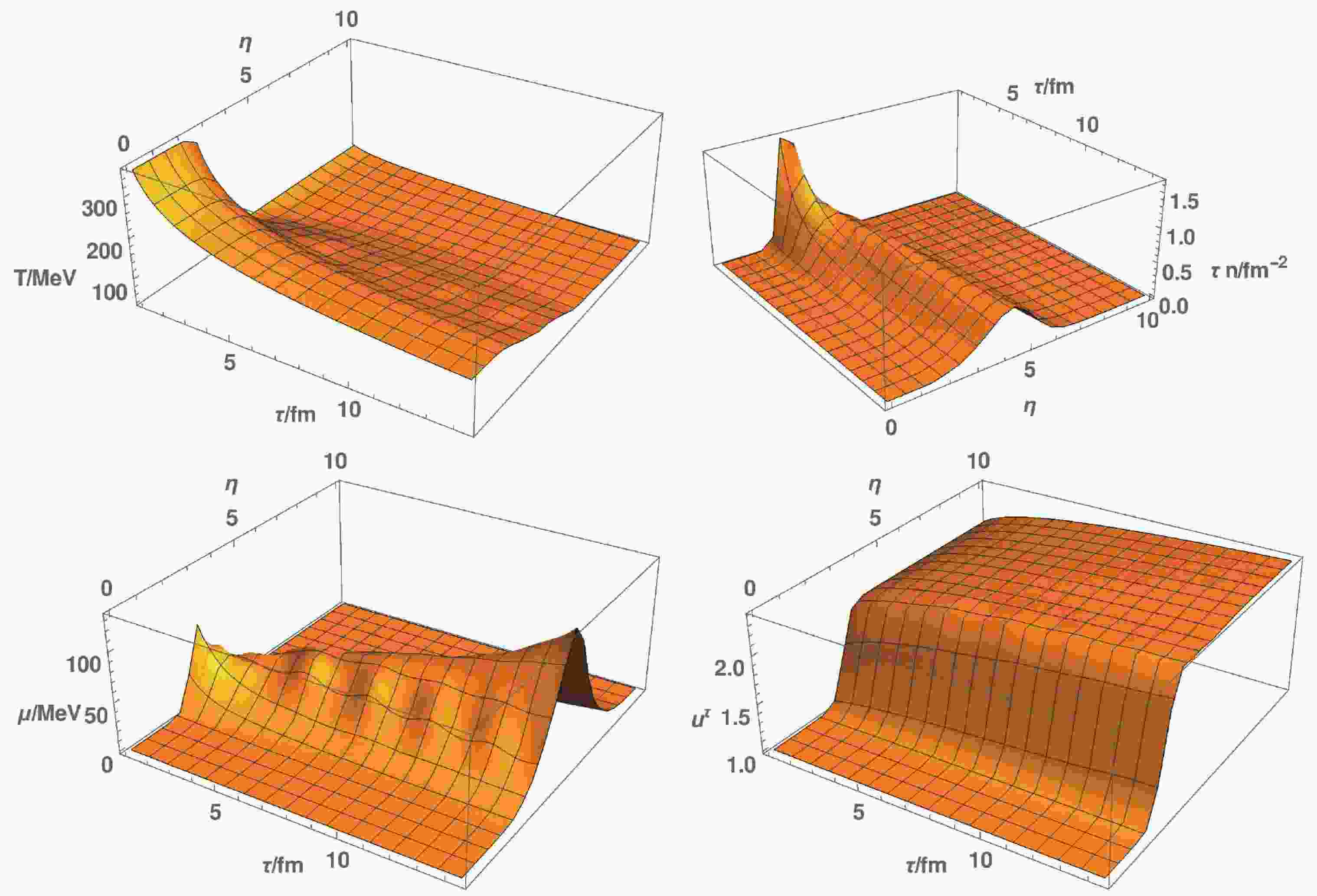
Let us first present numerical results without dissipation. In Fig. 1, we show the evolution of T,
$ n{\tau} $ , and$ {\mu} $ with$ T_{\max} = 360 \;{\rm{MeV}} $ ,$ T_ {\min} = 80 \;{\rm{MeV}} $ ,$ {\mu}_ {\max} = 80 \;{\rm{MeV}} $ , and$ u_{\max} = 2 $ . The value of$ T_ {\min} $ in our case was chosen to ensure stable numerical output. It is different from the case of actual heavy ion collisions with$ T_ {\min}\simeq0 $ . We will refer to$ n{\tau} $ as quark number density. The reason for using$ n{\tau} $ is that this is the total charge per rapidity with$ {\tau} $ from the volume factor. It is conserved in the boost invariant case. Note that both the temperature and quark number density decrease with increasing$ {\tau} $ due to longitudinal expansion. The peak of$ n{\tau} $ broadens and moves towards forward rapidity. The behavior of$ {\mu} $ follows a similar trend to n, except that it rises at late time with increasing$ {\tau} $ . The longitudinal flow builds up gradually with increasing$ {\tau} $ .
Figure 1. (color online) Top left: T as a function of
$ {\tau} $ and$ {\eta} $ . The temperature decreases with increasing$ {\tau} $ due to longitudinal expansion. Top right:$ n{\tau} $ as a function of$ {\tau} $ and$ {\eta} $ . The peak of$ n{\tau} $ broadens and moves towards forward rapidity. Bottom left:$ {\mu} $ as a function of$ {\tau} $ and$ {\eta} $ . The peak of chemical potential rises further, broadens, and moves towards forward rapidity, which can be understood from the combined effect of$ n{\tau} $ and T. Bottom right:$ u^{\tau} $ as a function of$ {\tau} $ and$ {\eta} $ . The longitudinal flow builds up gradually with increasing$ {\tau} $ . Parameters used:$ T_{\max} = 360 \;{\rm{MeV}} $ ,$ T_ {\min} = 80 \;{\rm{MeV}} $ ,$ {\mu}_ {\max} = 80 \;{\rm{MeV}} $ , and$ u_{\max} = 2 $ .The behavior of the peaks in
$ n{\tau} $ and$ {\mu} $ can be understood as a combined effect of T and n: at low$ {\mu} $ , we have$ {\mu} = \dfrac{n}{{\chi}} $ with$ {\chi}\sim T^2 $ . The decrease in the denominator is faster than the numerator, leading to the increase of$ {\mu} $ . The moving of the peak follows from the longitudinal flow that we impose on the initial condition. To illustrate this, in Fig. 2, we show$ n{\tau} $ at three different times for$ u_ {\max} = 1.5 $ and$ u_ {\max} = 2.5 $ , respectively. The peak corresponding to larger$ u_ {\max} $ moves faster towards forward rapidity. The broadening of the peak is correlated with the behavior in temperature. At$ {\tau} = 1{\rm{fm}} $ , the widths of the variation in temperature and chemical potential are set by$ {\Delta} $ . As the system cools down during longitudinal expansion, the width of the variation of temperature increases, which causes a similar increase in the width of peak of the chemical potential through their coupling in the hydrodynamic equations.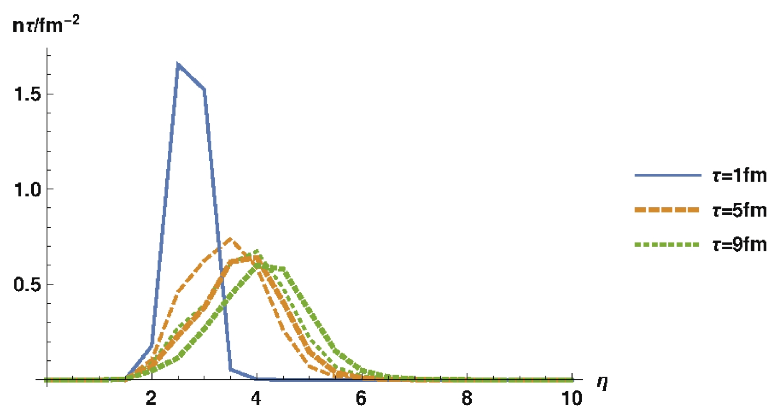
Figure 2. (color online)
$ n{\tau} $ as a function of$ {\eta} $ at three different values of$ {\tau} $ for$ u_ {\max} = 1.5 $ (thin lines) and$ u_ {\max} = 2.5 $ (thick lines). The initial profiles at$ {\tau} = 1{\rm{fm}} $ are the same. At later$ {\tau} $ , the case with larger longitudinal flow (larger$ u_ {\max} $ ) moves faster towards forward rapidity. Parameters used:$ T_{\max} = 360 \;{\rm{MeV}} $ ,$ T_ {\min} = 80 \;{\rm{MeV}} $ , and${\mu}_ {\max} = 80 \;{\rm{MeV}}$ .Next, we investigate the effect of dissipation. In Fig. 3, we show the evolution of
$ {\sigma} $ with and without dissipation. As the system cools down owing to longitudinal expansion, the chiral symmetry breaks through the growth of the sigma field. In the absence of dissipation, this occurs in an oscillatory fashion. Similar behavior is also observed in a boost invariant setting [28]. The effective relaxation can be understood as coming from longitudinal expansion. It would not exist in a static system, in which an off-equilibrium sigma field is expected to oscillate indefinitely. To analyze this further quantatively, we focused on the boost invariant case, in which the oscillatory behavior is known to exist [28]. We linearized the EOM of$ {\sigma} $ field in a background solution in which the$ {\sigma} $ field is set by the equilibrium value at local temperature and chemical potential. When the temperature drops significantly, the equilibrium value of sigma field corresponds to chiral symmetry breaking phase. The linearized EOM is given by
Figure 3. (color online)
$ {\sigma} $ as a function of$ {\tau} $ and$ {\eta} $ without dissipation (left) and with dissipative relaxation time$ {\tau}_{\rm rel} = 0.5{\rm{fm}} $ (right) starting from the same initial condition. In the absence of relaxation,$ {\sigma} $ rises in an oscillatory fashion. In the presence of sigma field dissipation, the oscillatory behavior is significantly reduced. Parameters used:$ T_{\max} = 360 \;{\rm{MeV}} $ ,$ T_ {\min} = 80 \;{\rm{MeV}} $ ,$ {\mu}_ {\max} = 80 \;{\rm{MeV}} $ , and$ u_{\max} = 2 $ .$ \partial_{\tau}^2{\delta}{\sigma}+\frac{1}{{\tau}}\partial_{\tau}{\delta}{\sigma}+\frac{{\delta}^2{\Omega}}{{\delta}{\sigma}^2}{\delta}{\sigma}+\frac{{\delta}^2{\Omega}}{{\delta}{\sigma}{\delta} T}{\delta} T+\frac{{\delta}^2{\Omega}}{{\delta}{\sigma}{\delta} {\mu}}{\delta} {\mu} = 0. $

(20) Given that
$ {\sigma} $ is at local minimum,$\dfrac{{\delta}^2{\Omega}}{{\delta}{\sigma}{\delta} T} = \dfrac{{\delta}^2{\Omega}}{{\delta}{\sigma}{\delta} {\mu}} = 0$ and$\dfrac{{\delta}^2{\Omega}}{{\delta}{\sigma}^2} > 0$ . The dynamics of$ {\delta}{\sigma} $ decouples from those of$ {\delta} T $ and$ {\delta}{\mu} $ :$ \partial_{\tau}^2{\delta}{\sigma}+\frac{1}{{\tau}}\partial_{\tau}{\delta}{\sigma}+\frac{{\delta}^2{\Omega}}{{\delta}{\sigma}^2}{\delta}{\sigma} = 0. $

(21) Clearly, by ignoring the middle term and considering
$ \dfrac{{\delta}^2{\Omega}}{{\delta}{\sigma}^2}\equiv k^2 $ as a slow-varying function of$ {\tau} $ , we obtain an approximate oscillatory solution${\delta}{\sigma}\sim {\rm e}^{{\rm i}k{\tau}}$ . The middle term is due to longitudinal expansion. It provides an effective friction term for$ {\delta}{\sigma} $ , with the effective relaxation time set by$ {\tau} $ . Physically, the dissipation arises from the loss of energy in fluid cells due to the longitudinal expansion.When dissipation is present, the oscillations of sigma field are significantly reduced. This is clearly visible in Fig. 4, which compares
$ {\sigma} $ , T, and$ {\mu} $ as a function of$ {\eta} $ at different times with and without dissipation. Interestingly, it is the non-dissipative case that corresponds to faster equilibration. Figure 4 suggests that the dissipation slows down the initial rise of sigma toward the chiral symmetry breaking minimum. The behavior of the sigma field is in agreement with the counterparts of temperature and chemical potential. The peak of the chemical potential is enhanced in the non-dissipative case. Analogous but milder enhancement also exists in temperature. These can be understood from conservation of charge and energy: in both cases, the charge and energy are conserved. The non-dissipative case converges more quickly to equilbrium, i.e., larger value of$ {\sigma} $ . Note that the thermodynamics of the quark sector is nothing but that of a free quark with constituent mass set by$ M_q = g{\sigma} $ . For the same values of T and$ {\mu} $ , the non-dissipative case (with larger$ M_q $ ) gives smaller charge density n and energy density$ {\epsilon} $ . To maintain the same n with the dissipative case,$ {\mu} $ has to rise further to compensate for the larger$ M_q $ . A similar rise in T is needed to maintain the same$ {\epsilon} $ with the non-dissipative case.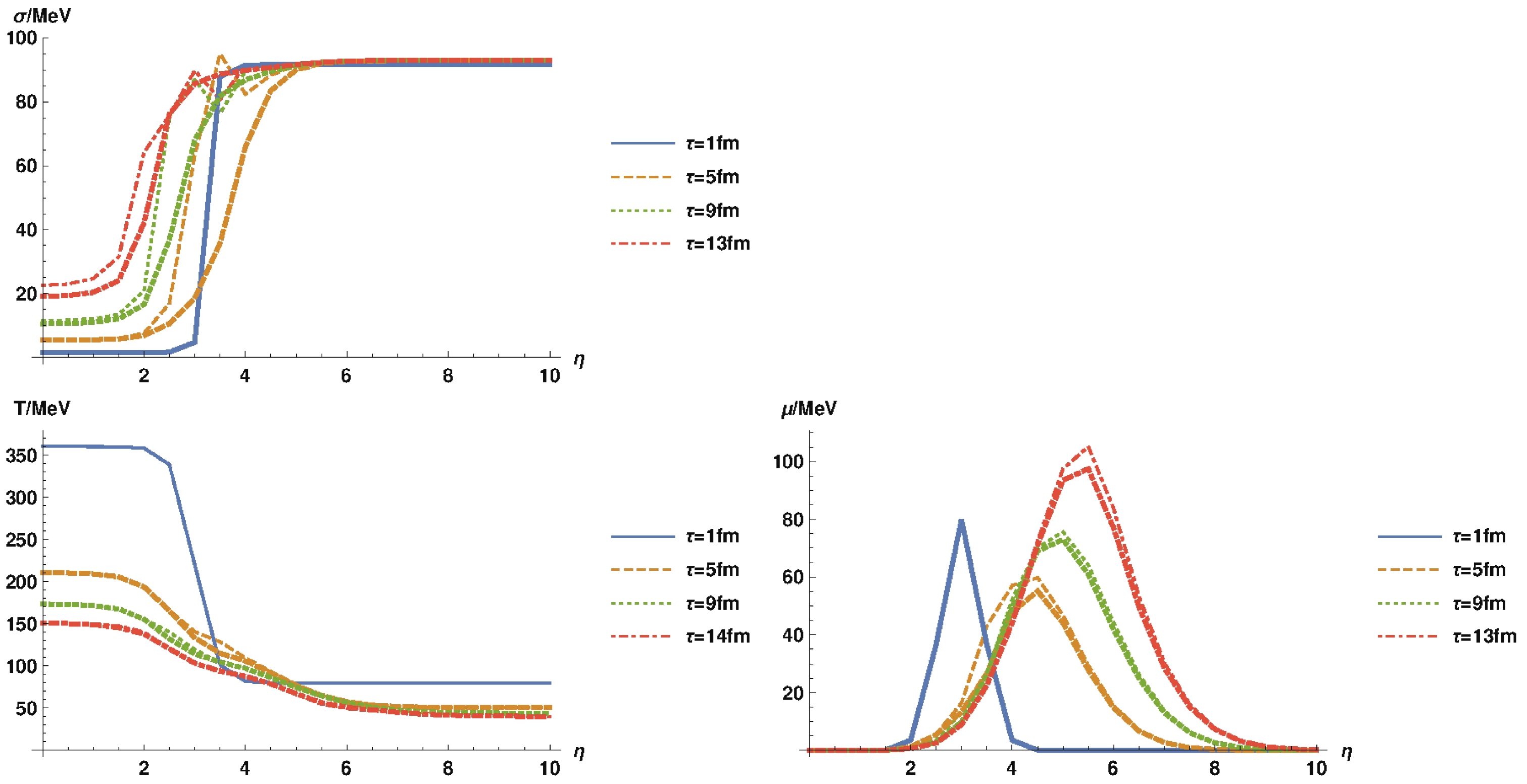
Figure 4. (color online)
$ {\sigma} $ (top), T (bottom left) , and$ {\mu} $ (bottom right) as a function of$ {\eta} $ at different values of$ {\tau} $ without (thin lines) dissipation and with dissipative relaxation time${\tau}_{\rm rel} = 0.5{\rm{fm}}$ (thick lines) starting with the same initial condition. The non-dissipative case corresponds to faster equilibration of$ {\sigma} $ and enhanced temperature and chemical potential. The behavior of T and$ {\mu} $ can be understood from the counterpart of$ {\sigma} $ and conservation of charge and energy (please, refer to the body text for further explanation). Parameters used:$ T_{\max} = 360 \;{\rm{MeV}} $ ,$ T_ {\min} = 80 \;{\rm{MeV}} $ ,$ {\mu}_ {\max} = 80 \;{\rm{MeV}} $ , and$ u_{\max} = 2 $ .It is also instructive to compare trajectories of fluid cells starting with the same initial rapidity for the cases with and without dissipation. We can trace the trajectories by solving the following equation:
$ u^{\tau}({\tau},{\eta}({\tau})) = \frac{{\rm d}{\tau}}{\sqrt{{\rm d}{\tau}^2-{\tau}^2{\rm d}{\eta}^2}} = \left(1-{\tau}^2\frac{{\rm d}{\eta}({\tau})}{{\rm d}{\tau}}\right)^{-1/2},$

(22) with the initial condition
$ {\eta}({\tau} = {\tau}_0) = {\eta}_0 $ for different$ {\eta}_0 $ . The LHS is known from the numerical solution of$ u^{\tau} $ . With the solution of Eq. (22), we can obtain different trajectories in the phase diagram. We show in Fig. 5 a comparison of trajectories with and without dissipation. The two cases are clearly distinguishable by the zig-zag shape present only in the case without dissipation. This is reminiscent of the oscillatory behavior in the sigma field in the absence of dissipation.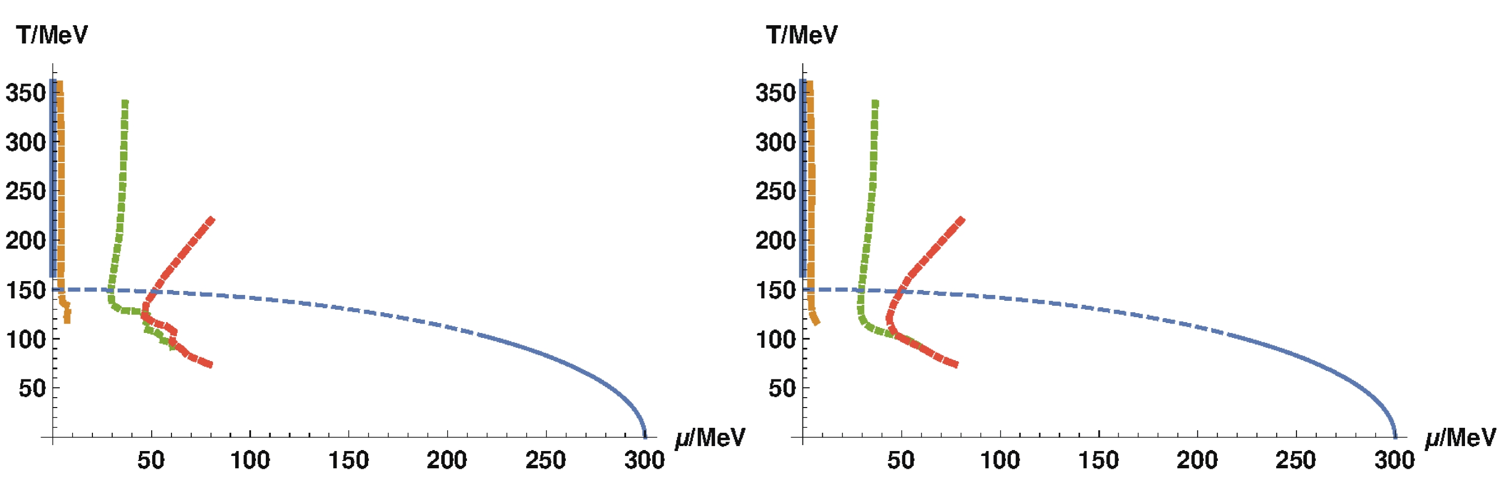
Figure 5. (color online) Trajectories of fluid cells starting with different initial rapidities for the case without dissipation (left) and with dissipative relaxation time
$ {\tau}_{\rm rel} = 0.5{\rm{fm}} $ (right). The initial rapidities for different trajectories are$ {\eta} = 1 $ ,$ {\eta} = 2 $ ,$ {\eta} = 2.5 $ , and$ {\eta} = 3 $ from left to right. The trajectories without dissipation are featured by zig-zag shape, which is reminiscent of the oscillatory behavior in the sigma field. The zig-zag shape is absent in the case with dissipation. The phase boundary is also shown in the plots with solid and dashed lines corresponding to first order and crossover transitions, respectively. Parameters used:$ T_{\max} = 360 \;{\rm{MeV}} $ ,$ T_ {\min} = 80 \;{\rm{MeV}} $ ,$ {\mu}_ {\max} = 80 \;{\rm{MeV}} $ , and$ u_{\max} = 2 $ .To have a closer look to the evolution of the sigma field, we show the sigma field in the fluid cell starting with
$ {\eta} = 3 $ for the case with and without dissipation in Fig. 6. We also use the equilibrium sigma field determined by local temperature and chemical potential as references for the corresponding cases. The cases with and without dissipation do not show significant difference for the equilibrium sigma field, but the difference in the actual sigma field is clearly visible in that the dissipative case shows reduced oscillation and delayed equilibration.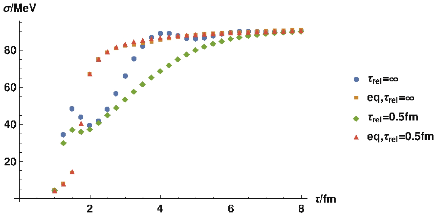
Figure 6. (color online)
$ {\sigma} $ as a function of$ {\tau} $ in the fluid cell starting with$ {\eta} = 3 $ for the cases with and without dissipation. Equilibrium$ {\sigma} $ determined by local temperature and chemical potential in the cell are also included for references. No significant effect of dissipation is seen in the equilibrium$ {\sigma} $ . The effect of dissipation is clearly visible from reduced oscillations and slow convergence to equilibrium in the actual$ {\sigma} $ . Parameters used:$ T_{\max} = 360 \;{\rm{MeV}} $ ,$ T_ {\min} = 80 \;{\rm{MeV}} $ ,$ {\mu}_ {\max} = 80 \;{\rm{MeV}} $ , and$ u_{\max} = 2 $ .To illustrate the role of the sigma field in the dynamics, we also compare the dynamics with and without the sigma field. For the former, we chose the non-dissipative case as a reference. For the latter, we used the standard hydrodynamic equations below:
$ \begin{aligned}[b] D_{\mu} T^{{\mu}{\nu}} = 0, \quad D_{\mu} J^{\mu} = 0. \end{aligned} $

(23) with
$ \begin{aligned}[b] &T^{{\mu}{\nu}} = ({\epsilon}+p)u^{\mu} u^{\nu}-pg^{{\mu}{\nu}}, \\ &J^{\mu} = nu^{\mu}. \end{aligned} $

(24) Here,
$ p = -{\Omega}_{\rm{eq}} $ and${\epsilon} = T\dfrac{\partial p}{\partial T}+{\mu} n-p$ . The equilibrium free energy$ {\Omega}_{\rm{eq}} = {\Omega}_{q\bar{q}} $ is evaluated at the minimum of$ {\Omega}_{q\bar{q}}+U $ for given temperature and chemical potential. While this is thermodynamically consistent, it is not consistent with the Lagrangian expressed in Eq. (1) because the vacuum potential U does not contribute to the stress tensor (24); it only plays a role in fixing the equilibrium value of$ {\sigma} $ . With this caveat in mind, we proceeded to solve Eq. (23) numerically with the following initial and boundary conditions:$ \begin{aligned}[b] T({\tau} = {\tau}_0,{\eta})& = \frac{T_{\max}-T_{\min}}{2}\tanh\frac{{\eta}_E-{\eta}}{{\Delta}}+\frac{T_{\max}+T_{\min}}{2}, \\ {\mu}({\tau} = {\tau}_0,{\eta})& = {\mu}_{\max}{\rm e}^{-({\eta}-{\eta}_E)^2/(2{\Delta}^2)}, \\ u^{\tau}({\tau} = {\tau}_0,{\eta})& = \frac{u_{\min}-u_{\max}}{2}\left[\tanh\frac{{\eta}_E-{\eta}}{{\Delta}}-\tanh\frac{{\eta}_E}{{\Delta}}\right]+u_{\min}, \\ \partial_{\eta} T({\tau},{\eta} = 0)& = \partial_{\eta}{\mu}({\tau},{\eta} = 0) = \partial_{\eta} u^{\tau}({\tau},{\eta} = 0) = 0.\\[-15pt] \end{aligned} $

(25) This choice ensures two cases having the same charge density initially. However, the total energy densities are different because the case without the sigma field does not include vacuum energy density. We solved Eq. (23) numerically and compared the hydrodynamic evolution with and without the sigma field.
In Fig. 7, we show the evolution of temperature and chemical potential for the two cases. The case without the sigma field shows an enhanced peak in
$ {\mu} $ and a moderate enhancement in T. The enhancement can be understood from the same mechanism discussed above. The case without the sigma field can be understood as instantaneous equilibration. In our case, it is equilibration toward chiral symmetry breaking minimum, giving rise to free quark with larger mass. Given that the evolution conserves n,$ {\mu} $ has to rise further to compensate for the larger mass to maintain the same charge density as in the case with the sigma field. A similar mechanism works for T, although there is a subtlety that the energy in the quark sector is not strictly conserved owing to the work by the sigma field. In Fig. 8, we compare the trajectories of fluid cells starting from different rapidities for the cases with and without the sigma field. The trajectories for the case without the sigma field bend toward region of larger$ {\mu} $ and T, which is consistent with the enhancement of$ {\mu} $ and T.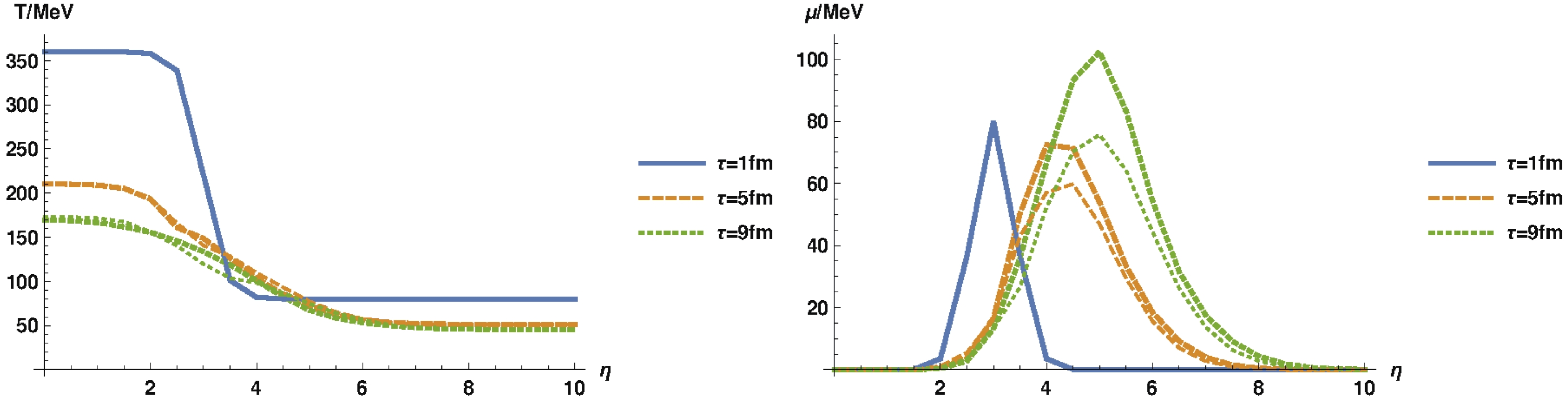
Figure 7. (color online) T (left) and
$ {\mu} $ (right) as a function of$ {\eta} $ at different values of t with (thin lines) and without (thick lines) sigma field. The case without sigma field shows an enhanced peak in$ {\mu} $ . A moderate enhancement in T is also present. This can be understood from conservation of charge and energy density (please, refer to the body text for further explanation). Parameters used:$ T_{\max} = 360 \;{\rm{MeV}} $ ,$ T_ {\min} = 80 \;{\rm{MeV}} $ ,$ {\mu}_ {\max} = 80 \;{\rm{MeV}} $ , and$ u_{\max} = 2 $ .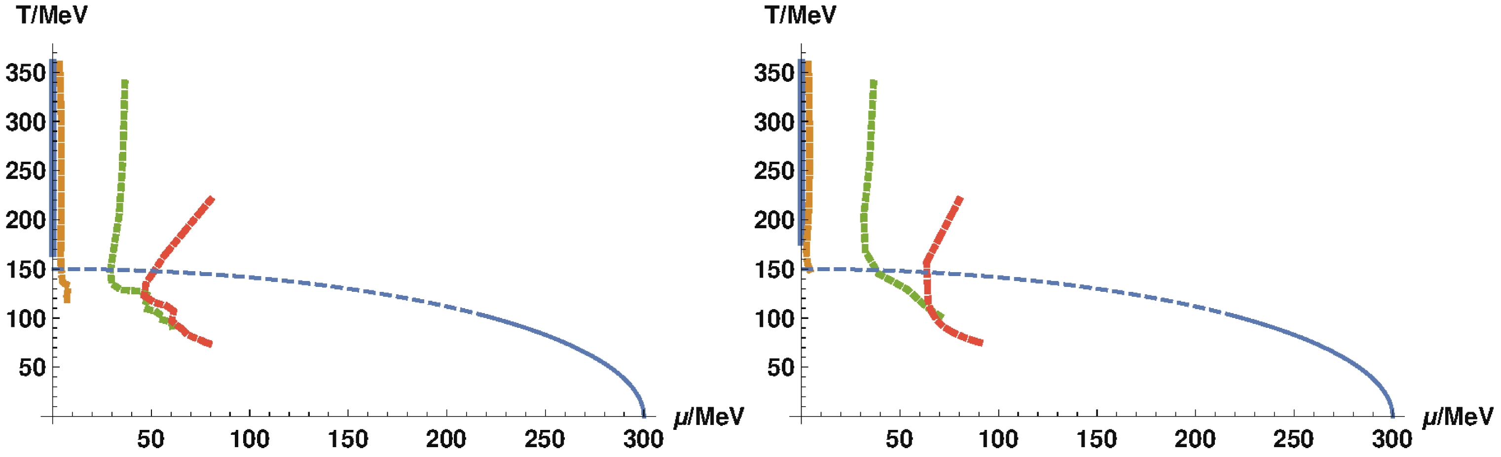
Figure 8. (color online) Trajectories of fluid cells starting with different initial rapidities for the case with (left) and without (right) non-dissipative sigma field. The initial rapidities for the different trajectories are
$ {\eta} = 1 $ ,$ {\eta} = 2 $ ,$ {\eta} = 2.5 $ , and$ {\eta} = 3 $ from left to right. The trajectories for the case without sigma field bend toward larger$ {\mu} $ and T. The phase boundary is also shown in the plots with solid and dashed lines corresponding to first order and crossover transitions, respectively. Parameters used:$ T_{\max} = 360 \;{\rm{MeV}} $ ,$ T_ {\min} = 80 \;{\rm{MeV}} $ ,$ {\mu}_ {\max} = 80 \;{\rm{MeV}} $ , and$ u_{\max} = 2 $ . -
We studied the coupled evolution of hydrodynamic fields and sigma field as the order parameter for chiral phase transition in the presence of nontrivial longitudinal flow using the chiral fluid dynamics model. We chose the initial condition with high temperature and low quark chemical potential, for which the phase transition in each fluid cell is a crossover. We found that the presence of longitudinal expansion provides an effective relaxation for the sigma field, resulting in equilibration in an oscillatory fashion. The oscillation is reduced when dissipation for the sigma field is present. However, the dissipation also seems to slow down the equilibration of the sigma field itself.
We also found that the quark density, which initially peaked at the boundary of the boost invariant region, moves toward forward rapidity, with the peak velocity correlated with the velocity of the longitudinal expansion. Meanwhile, the peak broadens during the evolution. As the system expands and cools down, the width of temperature variation also broadens, which causes a similar broadening in the quark chemical potential. The peak of the chemical potential rises as a result of simultaneous decrease of density and temperature. The peak is enhanced in the non-dissipative case compared to the dissipative case. A mild enhancement also occurs in terms of temperature. These follow from charge and energy conservation and different speeds of equilibration of the sigma field.
We also compared the coupled evolution of hydrodynamics and sigma fields with the standard hydrodynamics without the sigma field. It was found that the latter case leads to significant enhancement in the chemical potential and mild enhancement in the temperature. It can also be understood in terms of conservation of charge and energy and instantaneous equilibration of the sigma field in standard hydrodynamics.
While we restricted ourselves to the case of crossover, it is more interesting to generalize the current study to the case of first order phase transition, in which fluctuation is expected to play an essential role. It would be interesting to understand how longitudinal expansion and dissipation of the sigma field influence the first order phase transition. This will be addressed in future studies.
-
S.L. is grateful to Huichao Song for useful discussions.
Longitudinal dynamics from hydrodynamics with an order parameter
- Received Date: 2020-08-29
- Available Online: 2021-04-15
Abstract: We studied coupled dynamics of hydrodynamic fields and order parameter in the presence of nontrivial longitudinal flow using the chiral fluid dynamics model. We found that longitudinal expansion provides an effective relaxation for the order parameter, which equilibrates in an oscillatory fashion. Similar oscillations are also visible in hydrodynamic degrees of freedom through coupled dynamics. The oscillations are reduced when dissipation is present. We also found that the quark density, which initially peaked at the boundary of the boost invariant region, evolves toward forward rapidity with the peak velocity correlated with the velocity of longitudinal expansion. The peak broadens during this evolution. The corresponding chemical potential rises due to simultaneous decrease of density and temperature. We compared the cases with and without dissipation for the order parameter and also the standard hydrodynamics without order parameter. We found that the corresponding effects on temperature and chemical potential can be understood from the conservation laws and different speeds of equilibration of the order parameter in the three cases.


 DownLoad: