A comparison of condensate mass of QCD vacuum between Wilson line approach and Schwinger effect

I. INTRODUCTION

• I. INTRODUCTION
• II. MASS FROM CONDENSATION
• III. MASS FROM SCHWINGER EFFECT
• IV. CONCLUSIONS

Studying strong interactions in QCD shows the importance of vacuum condensate in both theory and phenomenology. Although the QCD sum rules constitute a basic tool in this issue, a strong alternative is needed for studying strongly coupled gauge theories in a non-perturbative formulation.

AdS/CFT is a holographic description in which a strongly coupled field theory on the boundary of the AdS space is mapped to the weakly coupled gravity theory in the bulk of AdS [1, 2]. In this approach, one starts from a five-dimensional effective field theory somehow motivated by string theory and tries to fit it to QCD as much as possible. The first conjecture is based on conformal field theories, but mass gap, confinement, and supersymmetry breaking could be included by considering some modifications in gravity duals [3-5].

A holographic model that represents the gluon condensation in a gravity background with Euclidean signature is expressed with the following action [6],

In the above action, $k$ denotes gravitational coupling in $5$-dimensions, $\mathcal{R}$ is the Ricci scalar, $L$ is the radius of the asymptotic ${\rm AdS}_5$ spacetime, and $\phi$ is a massless scalar that is coupled with the gluon operator on the boundary. To solve the Einstein equation and the dilaton equation of motion, one needs a suitable ansatz expressed as the following dilaton-wall solution in Euclidean spacetime [6],

where $\phi_0$ is a constant, $c = \dfrac{1}{z^4_c}$, and $z_{c}$ denotes the IR cutoff^①,

$x = x_1,x_2,x_3$ are orthogonal spatial boundary coordinates, and $z$ denotes the $5$-th dimension. The radial coordinate and $z = 0$ set the boundary. Expanding the dilaton profile near $z = 0$ will give,

where the parameter $c$ characterizes the QCD deconfinement transition; its value fulfills $0< c\leqslant 0.9\; {\rm GeV}^4$ [7-9]^②. The dilaton field is dual to a scalar operator and the metric is dual to the energy-momentum tensor of the dual field theory. Note that $\phi_0$ and c are the source and the parameter associated with the color confinement scale, respectively, according to the holographic dictionary [10] (refer to [11-13] for further discussion). The dilaton wall solution is related to the zero temperature case. Thus, it is appropriate to study the condensate of vacuum and its physics.

Another interesting phenomenon that could be studied in presence of the parameter $c$ is the Schwinger effect. By definition, the pair production in presence of an external electric field is known as Schwinger effect in non-perturbative QED [14]. Owing to this phenomenon, when the external field is strong enough, the virtual electron-positron pair becomes real particles. In other words, vacuum is destroyed in presence of such a field. Although this context had been first considered in QED, it is no longer restricted to it, and it was extended to QCD [15]. According to this mechanism, the vacuum decay can be considered in presence of a deformation parameter [16]. In addition, potential analysis of the Schwinger effect in presence of the condensation parameter was conducted in [17]. Therefore, we dismissed this part; the interested reader can refer to the mentioned references. However, the produced mass in such Schwinger effect mechanism was of our interest in this study.

This paper is organized as follows. In Section II, we follow the Wilson line calculation method based on [18] to discuss condensation. In Section III, by considering the standard form of brane embedding in the Schwinger effect holographic set up, we calculate $m$ as the produced mass; the effect of the condensation parameter is taken into account. Having results from both above approaches, we compare them. In Section IV, conclusions are presented.

II. MASS FROM CONDENSATION

• I. INTRODUCTION
• II. MASS FROM CONDENSATION
• III. MASS FROM SCHWINGER EFFECT
• IV. CONCLUSIONS

Before starting our calculations, we review the method reported in [18]. The reader can skip this part and continue from Eq. (11) in case they are familiar with this previous study. Condensation is associated with a five dimensional operator constructed from the quark ($q \bar{q}$) and gluon field ($G_{mn}$) as follows:

where $<\bar{q}q>$ denotes quark condensation, $\sigma^{mn}$ is an antisymmetric combination of matrices, and $g$ is a gauge coupling constant. Then, $m_0^2$ appears as a constant of proportionality in the parametrization. In fact, in analysis of condensation by QCD sum rules, $m_0^2$ appears between the zeroth moment of the quark-gluon distribution function and the first moment of the distribution function of quarks in the vacuum (see [19] for comprehensive discussion). Here, we avoid that calculation and follow holographic set up while we keep in our mind that $m_0^2$ is not mass of hadrons but is a coefficient (with $(mass)^2$ dimension) of quark condensate in the simplest quark-gluon mixed condensate. Let us consider a non-perturbative gauge invariant correlator as,

where $U_P (x_a,x_b)$ is a path-ordered Wilson line defined as,

where $\mu$ is running over the 4 dimensional indices and $l$ is a parameter of the path running from $0$ at $x = x_a$ to $1$ at $x = x_b$. The path is taken to be a straight line. If one sets [19]

then $m^2_0$ is given by the coefficient of $r^2$, with $r = |x_a-x_b|$, in the expansion of the function $Q$ as $r\longrightarrow 0$,

which holds in Euclidean space; in Minkowski space, it is modified by $r^2\longrightarrow -r^2$.

The author of the mentioned reference set an ansatz for computing the function $Q$ within gauge/string duality. The quark operators, the Wilson line on a four-manifold (which is the boundary of a 5-dimensional manifold), and the function $Q$ are given in terms of the area (in string units) of a surface in the 5-dimensional manifold by

Now let us go back to our case. As a conclusion from the above review, we can state that if we find $Q$ as a function of $r$, we can approximate the $m_0^2$ parameter.

Next, we will find the shape of the string describing the quark source. Let us consider the Nambu-Goto action:

where $\sigma^{\alpha}$ are the coordinates on the string worldsheet, $\mathcal{G}_{\mu\nu}$ is the space-time metric (Eq. (2)), $g_{\alpha\beta}$ is the induced metric, $\alpha'$ is the universal Regge slope, and the embedding of the string worldsheet in spacetime is

Then, from the background metric (Eq. (2)), dilaton field (Eq. (3)), and in static gauge $\sigma_{1} = t,0<t<\tau$, $\sigma_{2} = X_1 = x, -\dfrac{r}{2} < x< \dfrac{r}{2}$ one may obtain (In this calculation we wrote $\exp \dfrac{\phi(z)}{2} = \exp \log \left(\dfrac{1+cz^4}{1-cz^4}\right)^{\sqrt{\frac{3}{8}}} = \left(\dfrac{1+cz^4}{1-cz^4}\right)^\frac{\sqrt{\frac{3}{8}}}{\ln10} = \left(\dfrac{1+cz^4}{1-cz^4}\right)^{0.266}$, (recall that $\log A = \dfrac{\ln A}{\ln 10}$ and $\exp \dfrac{\ln A}{\ln 10} = A^{\frac{1}{\ln 10}}$) for this reason our (13) seems different with that of [8] while they are same. Also in our calculation only the first digit after the decimal point is taken into account so $(1+cz^4)^ {0.516}\approx \sqrt{1+cz^4}$. In addition one can set $\phi_0 = 0$ in (3) according to [8, 9]):

where we set the radius of spacetime $L = 1$. Then, the following relation should be satisfied:

From the boundary condition^④,

the constant value in the right hand side of Eq. (14) can be found. Thus, the solution of (14) is

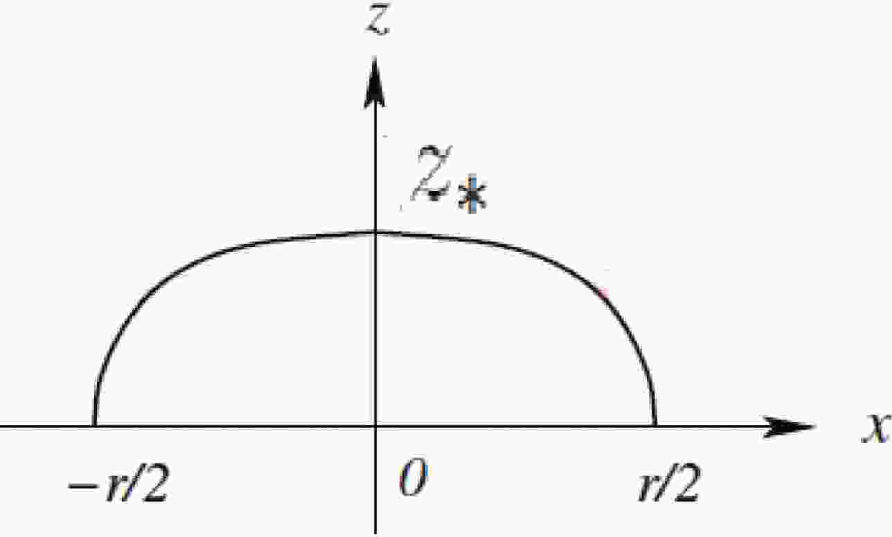
Applying a change of variable $u = \dfrac{z}{z_*}$, and using the boundary conditions shown in Fig. 1 as

Figure 1

Figure 1.  Surface of the 5- dimensional manifold with boundary at $z = 0$. The curved profile of the static string is stretched between quark sources from $-\dfrac{r}{2}$ and $\dfrac{r}{2}$. The surface is bounded between this and the straight Wilson line along x-axis; $z_\ast$ is the turning point of the string.

DownLoad: Full-Size Img PowerPoint

the shape of the string is expressed as

Therefore, at $z = 0$ and $-\dfrac{r}{2}<x<\dfrac{r}{2}$, Eq. (18) becomes

which is the length of the string. After describing the string shape, we need to calculate the renormalized area of the surface in Fig. 1.

To this end, we choose the gauge $\sigma_{1} = X_1 = x$ and $\sigma_{2} = z$, then from the action expressed by Eq. (11) and the string profile expressed by Eq. (18), we obtain^⑤

To regularize the above integral, one cut off the integral at $z = \epsilon$. Therefore, according to Eq. (20), the regularized solution to the integral is

$_{2}F_1$ is a hypergeometric function, and we subtract $\left(\dfrac{r}{2\pi \alpha' z_{*}}\left(\dfrac{1}{\epsilon}-a\right)\right)$ to address the power divergence, where $a$ is a constant that must be specified from renormalization conditions. The solution to the integral in Eq. (20) is given by the hypergeometric function:

Up to now, we found both $r$(Eq. (19)) and the action (Eq. (22)) describing the renormalized area. Relating them, we will obtain the behavior of the function $Q$ versus $r$. It is not clear how to carry out this. However, by considering two important limiting cases, long distances and short distances, we can analyze the behavior of the function.

We begin with Eq. (19). By considering $c_1 = cz_*^4$, one can check that $c_1\longrightarrow 0$ leads to long $r$, whereas $c_1\longrightarrow 1$ leads to short $r$. Expanding the right hand side of Eq. (19) around these two values of $c_1$ will show the behavior of $r$ at limiting cases. Thus, at short distances (we will denote this case by sd), the asymptotic behavior of Eq. (19) is given by the mathematical gamma function^⑥ as

and at long distances (we will denote this case by ld), the asymptotic behavior expressed by Eq. (19) is given by

Likewise, we expand Eq. (22) around $c_1\longrightarrow 0$ and $c_1\longrightarrow 1$ to find the behavior of the action at long distances and short distances, respectively. Then, at short distances, the action (22) behaves as,

and at long distances, the action in Eq. (22) behaves as

First, we should fix the value of $a$. According to the standard normalization of $Q$, we may impose the condition $Q(0) = 1$ [19], which gives $a = 0$.

Combining Eq. (25) with Eq. (23), we find the desired behavior of the function $Q$ at short distances as

where $R = r-\varepsilon$ and $\varepsilon$ is a small constant value. Finally, comparing Eq. (9) with Eq. (27), we may approximate mass at short distances as

Considering $\dfrac{1}{\alpha'} = 0.94$ and $c = 0.9 \;{\rm GeV}^4$ (from the fit to the slope of the Regge trajectories [4]), we can estimate $m_0^2$ as

According to the original phenomenological estimate based on the QCD sum rules [20], it is given by $m^2_0 = 0.8 \pm 0.2 \;{\rm GeV}^2$. Therefore, Eq. (29) shows an acceptable result. Notice that the condensation we are discussing in this study is a mixed condensate of quarks and gluons (Eq. (5)) but not exactly the gluon condensate $\alpha_s G^2$, whose values in different prior studies were extracted from phenomenology of QCD [21-27], mostly in the range of $0.024^4$- $0.07 \;{\rm GeV}^4$.

To address long distances we combine (26) with (24) and consider leading order of $r$; it shows that, at long distances, the function $Q$ decays exponentially, as it is expected in QCD:

where

In fact, in $4d$ QCD linear decay is expected, while Eq. (30) shows a faster decay according to the quadratic term $r^2$. It comes from the nature of the ${\rm GeV}^4$ modification of the background metric, which represents the condensation in gravity dual. Thus, such a dimension of $c$ leads to the exponential function of $Q$ as $-M^2 r^2$ rather than that of Ref. [18], which is $-Mr$ in presence of a modification parameter with $\;{\rm GeV}^2$ dimension. Notice that both dimensions of results are the same. To check the availability of this result, let us estimate the above $M$ with $\dfrac{1}{\alpha'} = 0.94$ and $c = 0.9 \;{\rm GeV}^4$, leading to

whose value is close to the pion mass. Similar to the result in [18], it is understood that, at long distances, the correlator is dominated by the lightest meson contribution. Having found an estimate for function $Q$ at short distances and its behavior at long distances, we close this section. Next, we study the produced mass by Schwinger effect in presence of condensation parameter.

III. MASS FROM SCHWINGER EFFECT

• I. INTRODUCTION
• II. MASS FROM CONDENSATION
• III. MASS FROM SCHWINGER EFFECT
• IV. CONCLUSIONS

Recall that the Schwinger effect is about vacuum decay in presence of an external electric field. In fact before vacuum decay, there is a potential barrier as $V_{\rm CP+SE}$, which is the sum of the Coulomb potential (CP) and static energy (SE). Once the external field is turned on, the total potential is $V_{\rm tot} = V_{\rm CP+SE}-Ex$ and includes the electrostatic potential between test particles (the virtual particles in vacuum that become real after decay of vacuum). In this relation $E$ is the external electric field and $x$ is the distance between particles. It is clear that increasing the field will suppress the potential barrier after a critical value; consequently, vacuum decays and virtual test particles become real [28-30].

As we mentioned before, the Schwinger effect potential analysis in presence of gluon condensation was studied in [17]. In this section, we followed mass production in the same mechanism. Consider a pair of virtual particles in vacuum that will become real particles in presence of a strong enough electric field. This procedure corresponds to a holographic potential barrier decay by gauge/gravity duality. If one considers the produced pair in the bulk, the mass value goes to infinity to avoid the divergent mass in a holographic way. A probe D3-brane attached to the test particles is located at an intermediate position $z_0$, as shown in Fig. 2 [31]. Thus, the mass formula is given by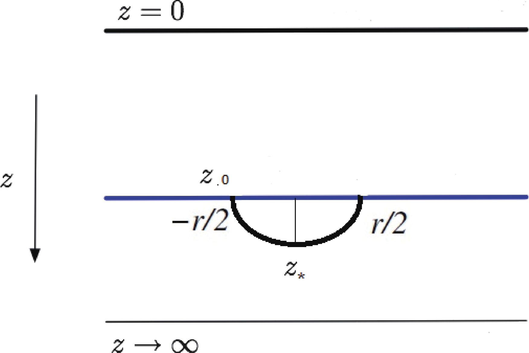

Figure 2

Figure 2.  Holographic set up to consider Schwinger effect test particles.

DownLoad: Full-Size Img PowerPoint

and with the induced metric on the string world-sheet and in static gauge, one may obtain

Combining this with Eq. (16), one may find

Applying a change of variable $y = \dfrac{z}{z_0}$ and $b = \dfrac{z_0}{z_*}$, Eq. (35) becomes

where we defined $c_1 = c z_*^4$. The integral in Eq. (36) is solvable analytically^⑦; however, given that $b<1$, we consider the leading term of $b$ in the solution and ignore others. Then, the solution is

We expand Eq. (37) near $c_1\longrightarrow 0$ and $c_1\longrightarrow 1$ to consider mass at long distances and short distances, respectively. At long distances, Eq. (37) becomes

and at short distances,

Combining Eq. (39) with Eq. (23), and Eq. (38) with Eq. (24), we may study mass at short distances and long distances, respectively. At long distances, the produced mass in Schwinger effect behaves as

which shows that with increasing $r$, the mass goes to zero. At short distances, the mass is given by

according to which any discussion on the produced mass in Schwinger effect significantly depends on the brane position $z_0$ in the bulk (in fact, given that $b = \dfrac{z_0}{z_*}$, having either $b$ or $z_0$ is enough). Although we have a phenomenological value for the parameter $c$ that can relate the distance of the produced pair and mass, $z_0 b^2$ always needs to be considered as a coefficient.

After deriving the mass formula in Schwinger effect in presence of condensation, it is interesting to compare the result with that of the previous section. Needless to say, what we found in the prior section is very different in its nature with respect to the Schwinger effect produced mass. Note that $m_0^2$, which appears in non-local and mixed condensates, is a constant of proportionality in the conventional parametrization. (Notice that even considering $m_0$ as exact value of quark mass could not be correct, as we mentioned in last section the value of this parameter has been estimated by original phenomenological estimate based on the QCD sum rules [20], it is given by $m^2_0 = 0.8 \pm 0.2 \;{\rm GeV}^2$.) So far, we have two different values by two different approaches; $m$from the Schwinger effect is exactly the mass of quark antiquark produced by vacuum decay. Although the responsible for vacuum decay and pair production is the external field $E$, parameter $c$ is in the background. On the one hand, if one accepts that in any mass production from vacuum some type of condensation appears, then the existence of the parameter $c$ in holographic Schwinger effect makes sense. On the other hand, we have $m_0^2$ from Wilson line calculation directly, meaning that the condensation is taking place based on $c$. Consequently, these two approaches are different in that what is responsible for mass production is also responsible in string and/or brane configuration, leading to different computations. However, they have the parameter $c$, which plays an important role in both approaches. The above explanations motivated us to compare $m$ and $m_0$. Considering both Eqs. (39) and (28), we can find the following approximate ratio:

As an example, let us consider the position of the probe brane in the bulk as $z_0 = \frac{z_*}{2}$. Knowing the mentioned position, we can find the fraction as

If we consider the intermediate position of the embedded brane in the bulk, it is interesting to study the behavior of $\dfrac{m_0}{m}$ schematically.

Figure 3 shows $\dfrac{m_0}{m}$ as a function of distance and $c$. The distance was considered $0< r< 1 \;{\rm fm}$ or $5\; {\rm GeV}^{-1}$; also, $c$ axis denotes a value $0< c\leqslant 0.9 \;{\rm GeV}^4$. Considering the parameter $c$ around our desired value, i.e., $0.9 \;{\rm GeV}^4$, with distance $r\simeq 0.14\; {\rm fm} = 0.7 \;{\rm GeV}^{-1}$, leads to $\dfrac{m_0}{m} = 1$. Increasing $r$ after this crucial value increases the ratio $\dfrac{m_0}{m}$ significantly. Notice that $r$ in string configuration corresponds to the diameter of a meson. As an example, let us consider the ratio $\dfrac{m_0}{m} = 1$ and $r\approx 2.6 \;{\rm GeV}^{-1} = 0.52\; {\rm fm}$ corresponding to the $J/\psi$ diameter. It leads to a very small value of the parameter $c\approx 0.005\; {\rm GeV}^4$. This value of $c$ gives us a near zero value of $m_0^2\approx 0.003 \;{\rm GeV}^2$ from Eq. (28). In comparison with Eq. (29), it is far from the acceptable value that fits QCD data. However, $J/\psi$ with $c\approx0.9 \;{\rm GeV}^4$ results in $\dfrac{m_0}{m}\approx 18$. Therefore, condensation of vacuum suppresses the Schwinger effect mass in an evident way. As a physics interpretation, one may relate that result. To the best of our knowledge, the Schwinger effect has not produced mass in experiments yet. Although the theory is clear and comprehensive enough (from QED to QCD and even higher dimensional objects), according to the nature of this phenomenon, it is not easy to reach the energy level that could destroy vacuum. By contrast, condensation (of gluons, quarks, etc.) does take place in hadrons structure, and the entire QCD structure is contained within hadrons. It seems universal in the QCD context. From this view, it makes sense that the Schwinger effect mass is suppressed by condensation of vacuum.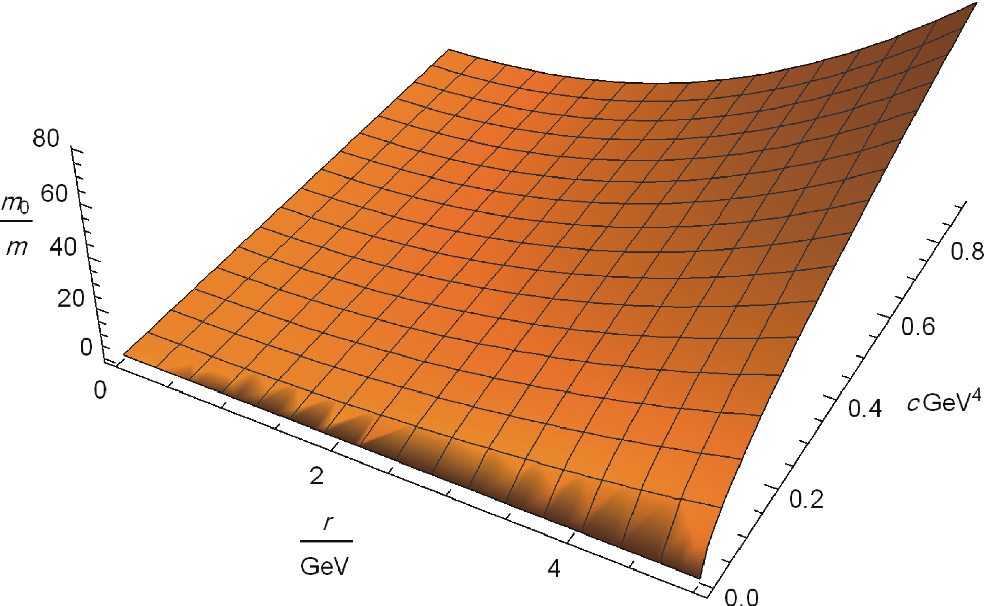

Figure 3

Figure 3.  (color online) Behavior of $\dfrac{m_0}{m}$ versus distance $({\rm GeV}^{-1})$ and parameter $c \;({\rm GeV}^4).$

DownLoad: Full-Size Img PowerPoint

IV. CONCLUSIONS

• I. INTRODUCTION
• II. MASS FROM CONDENSATION
• III. MASS FROM SCHWINGER EFFECT
• IV. CONCLUSIONS

Gluon condensation is an important issue given that it represents many phenomenological aspects of QCD. In this study, we considered dilaton wall background related to zero temperature to study vacuum condensation. First, we calculated $m^2_0$ by Wilson line calculation. Our results satisfy QCD data at both short distances and long distances. In the second step, we studied another mass production mechanism, the Schwinger effect, in the presence of gluon condensation, in which an external electric field is responsible for vacuum decay. These two mechanisms differ naturally in approaches and physics. However, since gluon condensation plays a role in both of them, it was in our interest to compare the results. We concluded by calculating the ratio $\dfrac{m_0}{m}$ as a function of $r$. We found that the produced mass via Schwinger effect is generally suppressed by condensation.

References