


 Abstract
 HTML
HTML Reference
 Related
 PDF
PDF


-
A measurement of the leptonic effective weak mixing angle,
$ \theta^\ell_{\rm{eff}} $ , is one of the most important topics in experimental particle physics. It is the key parameter in electroweak global fitting, and played a crucial role in predicting the mass of the Higgs boson with a precision of O(10) GeV. Going forward, it will continue to contribute in global fittings, and will aid in tests of the Standard Model and in searches for potential new physics beyond the Standard Model. At an energy scale of the Z boson mass ($ M_Z $ ),$ {\sin^2\theta_{{\rm{eff}}}^{\ell}} $ can be determined from measurements of parity violation in the neutral-current processes of fermion-antifermion scattering,$ f_i\bar{f_i}\rightarrow Z/\gamma^* \rightarrow f_j\bar{f_j} $ . One such measurement is the forward-backward asymmetry ($ A_{\rm FB} $ ), defined as$ A_{\rm FB} = \frac{N_{\rm F} - N_{\rm B}}{N_{\rm F} + N_{\rm B}}\,, $

(1) where
$ N_{\rm F} $ and$ N_{\rm B} $ are the number of forward and backward events, respectively. At lepton colliders, forward and backward events are defined according to the sign of$ \cos\theta $ , where$ \theta $ is the scattering angle between the outgoing fermion$ f_j $ and the incoming fermion$ f_i $ . The most precise determinations to date of$ {\sin^2\theta_{{\rm{eff}}}^{\ell}} $ at the Z pole are provided by the LEP and SLD collaborations [1], giving a combined result of$ 0.23153 \pm 0.00016 $ . The precisions of these measurements, achieved at the last generation of$ e^+e^- $ colliders, are limited by statistical uncertainties. Subsequent to the LEP/SLD era, measurements have been at hadron collider experiments, i.e., the Tevatron proton-antiproton collider, and the Large Hadron Collider (LHC) proton-proton collider, using$ A_{\rm FB} $ in the final states of Drell-Yan (DY)$ p\bar{p}/pp\rightarrow Z/\gamma^* \rightarrow \ell^+\ell^- $ processes, as a function of the di-lepton pair invariant mass. At hadron colliders, forward and backward events are defined in the Collins-Soper (CS) rest frame [2]. This is a special rest frame of the lepton pair, with the polar and azimuthal angles defined relative to the two hadron beam directions. The z axis is defined in the Z boson rest frame so that it bisects the angle formed by the momentum of either of the incoming hadrons and the negative of the momentum of the other hadron. The cosine of the polar angle$ \theta^{*} $ is defined by the direction of the outgoing lepton$ l^{-} $ relative to the$ \hat{z} $ axis in the CS frame and can be calculated directly from the laboratory frame lepton quantities by$ \cos\theta_{\rm CS}^{*} = c \, \frac{2(p^+_{1}p^-_{2} - p^-_{1}p^+_{2})} {m_{ll}\sqrt{m^2_{ll} + p^{2}_{{\rm T},ll}}} \,, $

(2) where the scalar factor c (either 1 or -1) is defined for the Tevatron and the LHC, respectively, as
$ c = \left\{ \begin{array}{l} \begin{array}{*{20}{l}} {1,}&{{\rm{for \;the \;Tevatron}}}\\ {{{\vec p}_{Z,ll}}/|{{\vec p}_{Z,ll}}|,}&{{\rm{for \;the \;LHC}} .} \end{array} \end{array} \right.$

(3) Thus, the sign of the z axis is defined as the proton beam direction for the Tevatron, and on an event-by-event basis as the sign of the lepton pair momentum with respect to the z axis in the laboratory frame for the LHC. The variables
$ p_{Z,ll} $ ,$ m_{ll} $ , and$ p_{{\rm T},ll} $ denote the longitudinal momentum, invariant mass and transverse momentum of the dilepton system, respectively, and,$ p^{\pm}_i = \frac{1}{\sqrt{2}}(E_i \pm p_{Z,i}) \,, $

(4) where the lepton (anti-lepton) energy and longitudinal momentum are
$ E_{1} $ and$ p_{Z,1} $ ($ E_{2} $ and$ p_{Z,2} $ ), respectively. The DY events are therefore defined as forward ($ \cos\theta_{\rm CS}^{*}>0 $ ) or backward ($ \cos\theta_{\rm CS}^{*}<0 $ ) according to the direction of the outgoing lepton in this frame of reference.Compared to lepton colliders, measurements at hadron colliders suffer from additional uncertainties on modeling the directions of the incoming fermions and antifermions in the initial state. Such uncertainties will dilute
$ A_{\rm FB} $ and reduce the sensitivity for the determination of$ {\sin^2\theta_{{\rm{eff}}}^{\ell}} $ . The degree of dilution at hadron colliders is modeled by the parton distribution functions (PDFs). At the Tevatron, fermions in the initial state of DY production are dominated by valence quarks. This allows us to make an assumption that the incoming quark of DY production is moving along the proton beam direction, as indicated in Eq. (3), while the direction of the incoming anti-quark is along the anti-proton beam. However, the contribution from sea-quark interactions is still as large as 10% at the Tevatron. The uncertainty of this dilution fraction, which is calculated using PDFs, will propagate into the uncertainty estimation of the$ {\sin^2\theta_{{\rm{eff}}}^{\ell}} $ measurement extracted from the$ A_{\rm FB} $ distribution. The combination of the D0 and CDF measurements at the Tevatron gives a result of$ 0.23179 \pm 0.00030({\rm{stat}})\pm 0.00017({\rm{PDF}}) \pm 0.00006 ({\rm{syst}}) $ [3], which shows a non-negligible PDF-induced uncertainty.The PDF dilution effect is even more significant at the LHC, since it is a proton-proton collider. Due to its completely symmetrical initial state, there is an equal probability of finding the incoming quark of DY production from either of the two proton beams. In order to distinguish forward from backward events in
$ pp $ collisions, the beam pointing to the same hemisphere as the Z boson reconstructed from final state leptons is assumed to be the one which provides the quark. This is motivated by the observation that the valence quarks inside the protons generally carry more energy than the antiquarks (or sea quarks) inside the protons. However, this assignment is only statistically correct, because it is possible for the sea quarks to have a larger fraction of momentum (x) of the incoming proton than the valence quarks. Furthermore, beyond leading order in the QCD interaction, quark-gluon and antiquark-gluon processes will contribute at next-to-leading order (NLO), and the gluon-gluon process will contribute at next-to-NLO (NNLO). These all affect the PDF dilution factor, whose magnitude depends on the precise modeling of the momentum spectra of all flavors of quarks and gluons involved in the Drell-Yan processes, which is more complicated than just modeling the total cross sections of valence quarks and sea quarks for the proton-antiproton case. Consequently, the PDF-induced uncertainty in the$ A_{\rm FB} $ measurement at the LHC is significantly larger than that at the Tevatron. The latest published measurement from the CMS collaboration gives a result of$ 0.23101\pm 0.00036({\rm{stat}}) \pm 0.00031 ({\rm{PDF}}) \pm $ $ 0.00024({\rm{syst}}) $ [4], in which the PDF uncertainty is about the same size as the statistical uncertainty. Measurements from LHCb and preliminary studies from the ATLAS collaboration using 8 TeV data have similar conclusions [5, 6].In the future high luminosity (HL) LHC era, the statistical uncertainty will be reduced as data accumulates. Thus, the PDF uncertainty will become the leading uncertainty that limits the precision in the determination of
$ {\sin^2\theta_{{\rm{eff}}}^{\ell}} $ . Studies have been done in the literature to discuss how to further reduce the PDF uncertainties relevant for precision electroweak measurements at the LHC [7]. Two experimental observables are essential to this task: one is the$ A_{\rm FB} $ of the DY pairs and the other is the lepton charge asymmetry$ A_\pm(\eta_{\ell}) $ in the$ W^\pm $ boson events. When$ A_{\rm FB} $ is used to simultaneously determine$ {\sin^2\theta_{{\rm{eff}}}^{\ell}} $ and to reduce PDF uncertainties, it will inevitably bring correlations. Such correlations have not been systematically considered in previous studies, as it is not expected to be important when the PDF-induced uncertainty does not dominate the overall uncertainty. In this article, we investigate the correlation between the two tasks of further reducing the PDF uncertainty and performing the precision determination of$ {\sin^2\theta_{{\rm{eff}}}^{\ell}} $ from measuring the same experimental observable$ A_{\rm FB} $ . We demonstrate the potential bias on the$ {\sin^2\theta_{{\rm{eff}}}^{\ell}} $ determination, and discuss possible solutions for the future LHC measurements. Note that the dilution effect at hadron colliders has a strong dependence on the Z boson rapidity. Therefore, if the weak mixing angle is extracted from the$ A_{\rm FB} $ spectrum observed as a function of Z boson rapidity, such as the measurement of the differential cross section of the Drell-Yan process from ATLAS [8], the bias might be different from that in the extraction using average$ A_{\rm FB} $ .The paper is organized as follows. In Section II, a brief review on using new data to update PDFs and to reduce the related uncertainties is presented. In Section III, we perform an exercise in updating the PDFs with
$ A_{\rm FB} $ at the LHC, and demonstrate its potential bias on the$ {\sin^2\theta_{{\rm{eff}}}^{\ell}} $ determination. In Section IV, we study how updating the PDFs with the lepton charge asymmetry$ A_\pm(\eta_{\ell}) $ measured at the LHC reduces the PDF uncertainties. In Section V, we study the implications of updating the PDFs with both$ A_{\rm FB} $ and$ A_\pm(\eta_{\ell}) $ data, and apply the error PDF Updating Method Package (ePump) optimization procedure to illustrate the complementary roles of the sideband$ A_{\rm FB} $ and$ A_\pm(\eta_{\ell}) $ observables in reducing the PDF uncertainty, and then to make the optimal choice of bin size of the experimental data used in the PDF-updating analysis. Finally, a summary is presented in Section VI. -
The two most commonly-used methods for extracting PDFs and their uncertainties from a global analysis of high-energy scattering data are the Monte Carlo method, used by NNPDF [9], and the Hessian method, as used in CT14HERA2 [10, 11]. In the Monte Carlo method, a statistical ensemble of PDF sets are provided, which are assumed to approximate the probability distribution of possible PDFs, as constrained from the global analysis of the data. In the Hessian method, a smaller number of error PDF sets are provided along with the central set which minimizes the
$ \chi^2 $ -function in a global analysis. These error PDF sets correspond to the positive and negative eigenvector directions in the space of PDF parameters. The most complete method for obtaining constraints from the new data on the PDFs would be to add the new data into the global analysis package and to do a full re-analysis. However, this is impractical for most users of the PDFs. A technique for estimating the impact of new data on the PDFs, without performing a full global analysis, is very useful. In the context of the Monte Carlo PDFs, the PDF reweighting method has become commonplace. This involves applying a weight factor to each of the PDFs in the ensemble [12-14] when performing ensemble averages. The PDF updating procedure will reduce the overall effective number of PDF replica in the ensemble. The impact of new data can also be estimated directly using Hessian PDFs [15-17], where it is called Hessian profiling, updating the eigenvectors within the Hessian approximation, which is faster and simpler. Note that both the Monte Carlo method and Hessian profiling are based on the original Monte Carlo PDFs or error sets, respectively. Therefore, the new data is assumed to be in general consistent with the PDF predictions before updating, so that the updated best-fit PDF set is not too different from the original best fit. If a large deviation is found between the new data and the original theory predictions, a full analysis of PDF global fitting is needed.The theoretical predictions in this work are computed using the ResBos [18] package at next-to-leading order (NLO) plus next-to-next-leading log (NNLL) in QCD, in which the canonical scales are used [19, 20]. The CT14HERA2 central and error PDFs [10, 11] are used in this analysis.
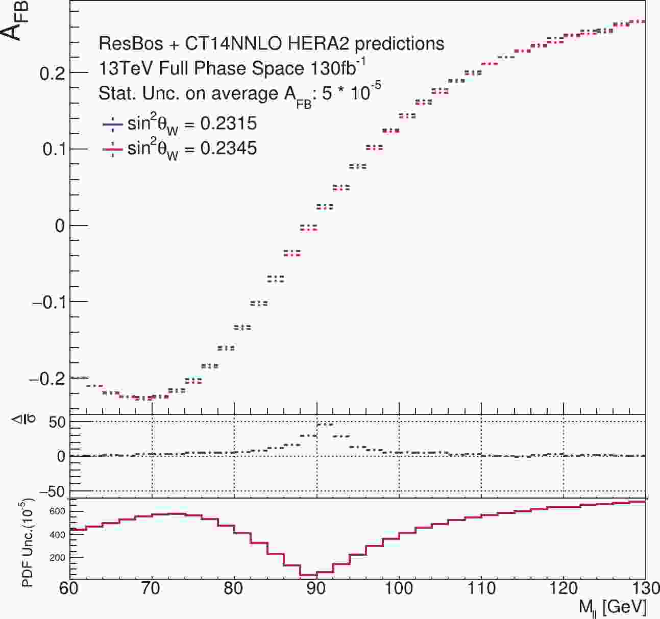
$ A_{\rm FB} $ as a function of dilepton mass ($ M_{\ell\ell} $ ) at LHC is sensitive both to$ {\sin^2\theta_{{\rm{eff}}}^{\ell}} $ and to PDF modeling. Fig. 1 shows the$ A_{\rm FB} $ distributions of two separated$ {\sin^2\theta_{{\rm{eff}}}^{\ell}} $ values of 0.2315 and 0.2345, their difference, and the PDF uncertainties as functions of the di-lepton invariant mass for$ \sqrt{s} = 13 $ TeV$ pp $ collisions at the LHC. The two values of$ {\sin^2\theta_{{\rm{eff}}}^{\ell}} $ are arbitrarily chosen to be far separated in order to clearly reveal their different predictions of$ A_{\rm FB} $ . When$ A_{\rm FB} $ from a new data set is used in the PDF updating procedure, it is assumed to be consistent with the current theory predictions. This means that$ {\sin^2\theta_{{\rm{eff}}}^{\ell}} $ , on which$ A_{\rm FB} $ depends, is considered to have the same value as determined from existing experimental measurements, even if a different value of$ {\sin^2\theta_{{\rm{eff}}}^{\ell}} $ is used in generating the pseudo-data. As a result, a simple PDF updating procedure will forcibly absorb the difference in$ {\sin^2\theta_{{\rm{eff}}}^{\ell}} $ into the PDFs, which will bias the determination of both the updated PDFs and the extracted$ {\sin^2\theta_{{\rm{eff}}}^{\ell}} $ . The size of the bias depends on how large the difference is between the current accepted value of$ {\sin^2\theta_{{\rm{eff}}}^{\ell}} $ (used in the theory prediction) and the value used in the generation of the pseudo-data, which will be quantitatively discussed in the following sections. An important thing to note is that$ A_{\rm FB} $ is more sensitive to$ {\sin^2\theta_{{\rm{eff}}}^{\ell}} $ in the Z-pole region, while the PDF-induced uncertainty becomes more significant when$ M_{\ell\ell} $ moves to higher or lower regions. The difference in sensitivities of the regions suggests a method to reduce the correlations. The work presented in Ref. [7] was done using the Monte Carlo reweighting method, with NNPDF PDFs, and was based on the hypothesis that the above-mentioned correlation is negligible. In this work, we instead use the software package$ {\texttt{ePump}}$ (error PDF Updating Method Package), which can update any given set of Hessian PDFs obtained from an earlier global analysis [21].
Figure 1. (color online)
$A_{\rm FB}$ theory prediction as a function of$M_{\ell\ell}$ at the 13 TeV LHC. The luminosity assumed in the samples is 130 fb$^{-1}$ . No fiducial acceptance selections are applied. The$\Delta/\sigma$ in the middle panel is defined as$(A_{\rm FB}[\sin^2 \theta _{{\rm{eff}}}^{\ell} = 0.2345] - A_{\rm FB}[\sin^2 \theta _{{\rm{eff}}}^{\ell} = 0.2315]) / \sigma$ , where$\sigma$ is the statistical uncertainty of the event samples in that mass bin. The bottom panel shows the magnitude of PDF-induced uncertainty of$A_{\rm FB}$ , predicted by the CT14HERA2 error PDFs, at the 68% CL. -
In this section, we quantitatively examine how the PDF-induced uncertainty in the determination of
$ {\sin^2\theta_{{\rm{eff}}}^{\ell}} $ can be reduced by applying the Hessian updating method, via$ {\texttt{ePump}}$ , and study the correlation mentioned above. First, we consider the case of using the$ A_{\rm FB} $ data spanning the full range of$ M_{\ell\ell} $ , from 60 to 130 GeV. Second, we consider the case of using only the$ A_{\rm FB} $ sideband spectrum, where events with$ M_{\ell\ell} $ from 80 to 100 GeV are excluded.In order to perform the PDF update,
$ {\texttt{ePump}}$ requires two sets of inputs: data templates and theory templates. The data templates provide$ A_{\rm FB} $ distributions with their uncertainties. The theory templates consist of the theory predictions for the$ A_{\rm FB} $ from the original PDF error sets. The output of$ {\texttt{ePump}}$ consists of an updated central and Hessian eigenvector PDFs, representing the result that would be obtained from a full global re-analysis that includes the new data. As an additional benefit,$ {\texttt{ePump}}$ can also output the updated predictions and uncertainties for any other observables of interest without having to recalculate using the updated PDFs. For more details about the use of$ {\texttt{ePump}}$ , see Ref. [15].For the DY samples, each lepton flavor channel-electron and muon - has 250 million events in the mass range of
$ 60 $ $ \leqslant M_{\ell\ell} \leqslant 130 $ GeV. This sample size corresponds to an integrated luminosity of roughly 130 fb$ ^{-1} $ , which is reasonably close to the total data collected by the ATLAS detector during the LHC Run 2. The pseudo-data is modeled using the$ {\texttt{CT14HERA2}}$ central PDFs. Nominal theory-template samples consist of the central and (56) error PDF predictions, generated using the$ {\texttt{CT14HERA2}}$ error PDFs sets. In the theory templates,$ {\sin^2\theta_{{\rm{eff}}}^{\ell}} $ is set to be 0.2315, which is the value determined by the LEP and SLD collaborations. In the pseudo-data,$ {\sin^2\theta_{{\rm{eff}}}^{\ell}} $ is set to be 0.2324 in order to examine the effects of an offset or pull in the new data. The difference is deliberately chosen to be three times the uncertainty of the$ {\sin^2\theta_{{\rm{eff}}}^{\ell}} $ measurement as determined at hadron colliders [3]. To mimic the experimental acceptance, a set of ATLAS detector-like event selections are further applied to the pseudo-data and the nominal theory samples:● Each lepton is required to have transverse momentum
$ p_T $ $ \geqslant $ 25 GeV.● Lepton pseudo-rapidity is limited by
$ |\eta_{\ell}| $ $ < $ 4.9.● Events are denoted as
$ {\rm CC} $ (central-central) if both leptons have$ |\eta_{\ell}| \leqslant 2.5 $ , and$ {\rm CF} $ (central-forward) if one lepton has$ |\eta_{\ell}| \leqslant 2.5 $ and the other has$ 2.5<|\eta_{\ell}|<4.9 $ . The$ {\rm CC} $ events correspond to doubling the integrated luminosity with respect to the$ {\rm CF} $ events, since both the dielectron and dimuon channels contribute to the$ {\rm CC} $ events, while only the dielectron channel has$ {\rm CF} $ events at the ATLAS detector.● The Z-pole region is defined as dilepton invariant mass satisfying
$ 80 \leqslant M_{\ell\ell} \leqslant 100 $ GeV. The sideband region is defined as$ 60 < M_{\ell\ell} < 80 $ GeV and$ 100< $ $ M_{\ell\ell}<130 $ GeV.● The forward-backward asymmetry
$ A_{\rm FB} $ is measured in a 2 GeV mass bin size.Note that the pseudo-data were treated as coming from just one “experiment”, but in practice both ATLAS and CMS would be sources of input data for fitting. For the CMS case, a CF channel measurement would be difficult due to a limited detector acceptance, while the CC events could be fully used as input.
-
First, we will update the PDFs using the full mass range
$ A_{\rm FB} $ . It is expected that the PDF-induced uncertainty on$ A_{\rm FB}(M_{\ell\ell}) $ will be reduced after updating the original PDFs with the inclusion of the pseudo-data. Note that the pseudo-data and theory prediction are generated by the same CT14HERA2 PDFs. If the correlation between$ {\sin^2\theta_{{\rm{eff}}}^{\ell}} $ and the PDF updating is negligible, we expect no changes in the central value of$ A_{\rm FB} $ as predicted by the PDFs after updating, compared to that given in the original theory prediction.The predicted
$ A_{\rm FB} $ distributions ($ {\sin^2\theta_{{\rm{eff}}}^{\ell}} = 0.2315 $ ) and the associated PDF-induced uncertainties, before and after the PDF updating by using the full mass range of the pseudo-data ($ {\sin^2\theta_{{\rm{eff}}}^{\ell}} = 0.2324 $ ), are depicted in Figs. 2 and 3 for the$ {\rm CC} $ and$ {\rm CF} $ event samples, respectively. As shown in the bottom panels of the figures, the PDF-induced uncertainties on the predicted$ A_{\rm FB} $ are significantly reduced after the updating procedure. This finding is consistent with the conclusion of Ref. [7]. However, as also shown in the middle panels of the figures, the central values of$ A_{\rm FB} $ differ before and after the updating, particularly in the Z-pole region. The difference is more significant in$ {\rm CF} $ events than for$ {\rm CC} $ . When the$ {\sin^2\theta_{{\rm{eff}}}^{\ell}} $ of the pseudo-data has a value different from its value in the theory predictions, the existing PDF model (i.e., CT14HERA2 PDFs, in this study) no longer describes the new data in a consistent way. As a result, the PDF updating procedure would forcibly convert this bias, which originated from a different value of$ {\sin^2\theta_{{\rm{eff}}}^{\ell}} $ , into an updated central PDF set. The averaged$ A_{\rm FB} $ values in the Z-pole region in the pseudo-data and theory predictions, before and after PDF updating, are numerically presented in Tables 1, 2 and 3, for the$ {\rm CC} $ ,$ {\rm CF} $ and$ {\rm CC+CF} $ events. The$ {\rm CF} $ events have higher sensitivity to the$ A_{\rm FB} $ . For example, as given in the third line of Table 2, the PDF uncertainty can be decreased from 0.00118 to 0.00055, a reduction of more than 50%. Meanwhile, the bias on$ A_{\rm FB} $ , originating from the PDF updating, can be as large as$ \Delta = -0.00108 $ , as shown in the same line of the table. As we pointed out, there should be no difference in the central value of$ A_{\rm FB} $ before and after an unbiased updating, because the pseudo-data and theory templates are generated with the same PDF sets. This bias, which is larger than the statistical uncertainty shown in the third column, indicates that much of the effect of the shift in$ {\sin^2\theta_{{\rm{eff}}}^{\ell}} $ has been absorbed into the updated PDFs.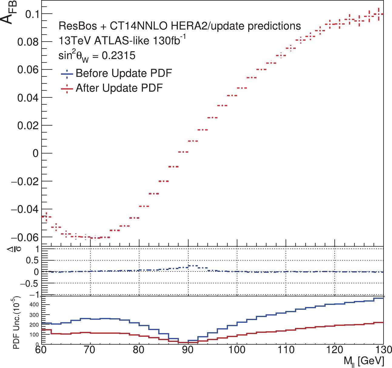
Figure 2. (color online) Predicted
$A_{\rm FB}$ distributions ($\sin^2 \theta _{{\rm{eff}}}^{\ell} =0.2315$ ) and associated PDF-induced uncertainties, before and after PDF updating using the full mass range of the pseudo-data ($\sin^2 \theta _{{\rm{eff}}}^{\ell} =0.2324$ ). Only${\rm CC}$ events are considered.$\Delta/\sigma$ in the middle panel is defined as ($A_{\rm FB}$ [before] -$A_{\rm FB}$ [after])/$\sigma$ , where$\sigma$ is the statistical uncertainty of the samples in that bin. The bottom panel shows the magnitude of the PDF-induced uncertainty of$A_{\rm FB}$ , predicted by the CT14HERA2 error PDFs, at 68% CL., before and after updating the PDFs.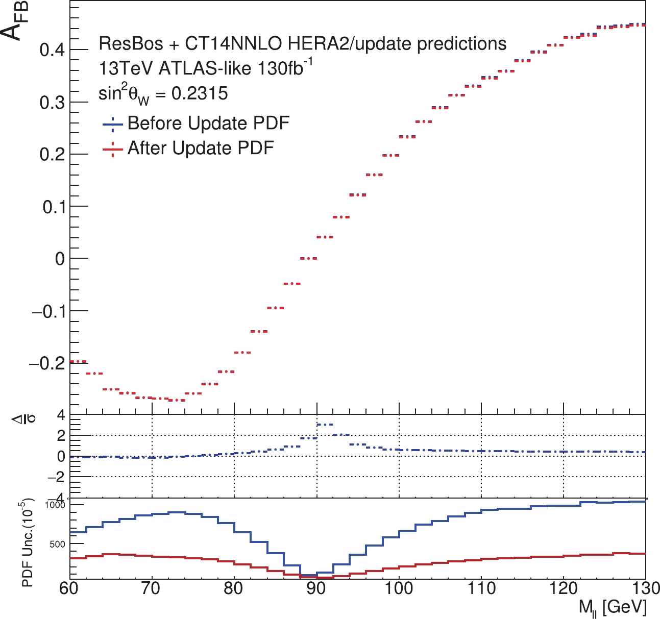
Figure 3. (color online) Similar to Fig. 2, but for
${\rm CF}$ events only.Update using ${\rm CC}$ with full

$A_{\rm FB}$ 

average $A_{\rm FB}$ at Z pole

PDF uncertainty Statistical uncertainty pseudo-data $\sin^2 \theta _{{\rm{eff}}}^{\ell} = 0.2324$ 

in ${\rm CC}$ events

0.00825 − 0.00008 in ${\rm CF}$ events

0.03983 − 0.00017 in ${\rm CC+CF}$ events

0.01368 − 0.00007 theory prediction in ${\rm CC}$ events,

$\sin^2 \theta _{{\rm{eff}}}^{\ell} = 0.2315$ 

before update 0.00873 0.00038 0.00008 after update 0.00867 0.00019 0.00008 $\Delta$ [after-before]

−0.00006 − − theory prediction in ${\rm CF}$ events,

$\sin^2 \theta _{{\rm{eff}}}^{\ell} = 0.2315$ 

before update 0.04220 0.00118 0.00017 after update 0.04201 0.00092 0.00017 $\Delta$ [after-before]

−0.00019 − − theory prediction in ${\rm CC+CF}$ events,

$\sin^2 \theta _{{\rm{eff}}}^{\ell} = 0.2315$ 

before update 0.01449 0.00053 0.00007 after update 0.01440 0.00031 0.00007 $\Delta$ [after-before]

−0.00009 − − Table 1. (color online) Average
$A_{\rm FB}$ in the Z-pole region in the pseudo-data and theory predictions. The PDF updating was done using the full mass range$A_{\rm FB}$ spectrum from the${\rm CC}$ events of pseudo-data ($\sin^2 \theta _{W}=0.2324$ ). The statistical uncertainty corresponds to the data sample with an integrated luminosity of 130 fb$^{-1}$ .Update using ${\rm CF}$ with full

$A_{\rm FB}$ 

average $A_{\rm FB}$ at Z pole

PDF uncertainty Statistical uncertainty pseudo-data $\sin^2 \theta _{{\rm{eff}}}^{\ell} = 0.2324$ 

in ${\rm CC}$ events

0.00825 − 0.00008 in ${\rm CF}$ events

0.03983 − 0.00017 in ${\rm CC+CF}$ events

0.01368 − 0.00007 theory prediction in ${\rm CC}$ events,

$\sin^2 \theta _{{\rm{eff}}}^{\ell} = 0.2315$ 

before update 0.00873 0.00038 0.00008 after update 0.00856 0.00026 0.00008 $\Delta$ [after-before]

−0.00017 − − theory prediction in ${\rm CF}$ events,

$\sin^2 \theta _{{\rm{eff}}}^{\ell} = 0.2315$ 

before update 0.04220 0.00118 0.00017 after update 0.04112 0.00055 0.00017 $\Delta$ [after-before]

−0.00108 − − theory prediction in ${\rm CC+CF}$ events,

$\sin^2 \theta _{{\rm{eff}}}^{\ell} = 0.2315$ 

before update 0.01449 0.00053 0.00007 after update 0.01416 0.00032 0.00007 $\Delta$ [after-before]

−0.00033 − − Table 2. Average
$A_{\rm FB}$ in the Z-pole region in the pseudo-data and theory predictions. The PDF updating is done using the full mass range$A_{\rm FB}$ spectrum from the${\rm CF}$ events of pseudo-data ($\sin^2 \theta _{{\rm{eff}}}^{\ell} =0.2324$ ). The statistical uncertainty corresponds to the data sample with an integrated luminosity of 130 fb$^{-1}$ .Update using ${\rm CC}$ +

${\rm CF}$ with full

$A_{\rm FB}$ 

average $A_{\rm FB}$ at Z pole

PDF uncertainty Statistical uncertainty pseudo-data $\sin^2 \theta _{{\rm{eff}}}^{\ell} = 0.2324$ 

in ${\rm CC}$ events

0.00825 − 0.00008 in ${\rm CF}$ events

0.03983 − 0.00017 in ${\rm CC+CF}$ events

0.01368 − 0.00007 theory prediction in ${\rm CC}$ events,

$\sin^2 \theta _{{\rm{eff}}}^{\ell} = 0.2315$ 

before update 0.00873 0.00038 0.00008 after update 0.00853 0.00018 0.00008 $\Delta$ [after-before]

−0.00020 − − theory prediction in ${\rm CF}$ events,

$\sin^2 \theta _{{\rm{eff}}}^{\ell} = 0.2315$ 

before update 0.04220 0.00118 0.00017 after update 0.04105 0.00054 0.00017 $\Delta$ [after-before]

−0.00115 − − theory prediction in ${\rm CC+CF}$ events,

$\sin^2 \theta _{{\rm{eff}}}^{\ell} = 0.2315$ 

before update 0.01449 0.00053 0.00007 after update 0.01411 0.00025 0.00007 $\Delta$ [after-before]

−0.00038 Table 3. Average
$A_{\rm FB}$ in the Z-pole region in the pseudo-data (with$\sin^2 \theta _{W}=0.2324$ ) and theory predictions (with$\sin^2 \theta _{W}=0.2315$ ). The PDF updating is done using the full mass range$A_{\rm FB},$ from the${\rm CC}$ ,${\rm CF}$ or${\rm CC+CF}$ events of pseudo-data. The statistical uncertainty corresponds to the data sample with an integrated luminosity of 130 fb$^{-1}$ .To estimate the impact on the determination of
$ {\sin^2\theta_{{\rm{eff}}}^{\ell}} $ in the Z-pole mass region, we express the average$ A_{\rm FB} $ approximately as a linear function of$ {\sin^2\theta_{{\rm{eff}}}^{\ell}} $ in this region, written as$ A_{\rm FB} \simeq k \cdot {\sin^2\theta_{{\rm{eff}}}^{\ell}} + b \, , $

(5) where the values of the parameters k and b are listed in Table 4, for
$ {\rm CC} $ ,$ {\rm CF} $ and$ {\rm CC+CF} $ event samples, respectively. The linear approximation and the values of the slope and offset are acquired using the ResBos [18] generator. The potential bias due to the non-linearity between$ A_{\rm FB} $ and$ {\sin^2\theta_{{\rm{eff}}}^{\ell}} $ , and those higher order corrections, lead to the shift in the central value of$ {\sin^2\theta_{{\rm{eff}}}^{\ell}} $ to be smaller than 0.00010, and have a negligible effect on the statistical uncertainty estimation [3].slope factor k offset factor b ${\rm CC}$ events

−0.531 0.132 ${\rm CF}$ events

−2.512 0.623 ${\rm CC+CF}$ events

−1.110 0.275 Table 4. Simple linear functions between
$\sin^2 \theta _{{\rm{eff}}}^{\ell} $ and the observed$A_{\rm FB}$ around the Z pole, predicted by ResBos with CT14NNLO PDFs, for the${\rm CC}$ ,${\rm CF}$ and${\rm CC+CF}$ event samples.One can roughly estimate the bias and the PDF-induced uncertainty on the determination of
$ {\sin^2\theta_{{\rm{eff}}}^{\ell}} $ , derived from the biased$ A_{\rm FB} $ measurement, using the following simplified relation:$ \Delta {\sin^2\theta_{{\rm{eff}}}^{\ell}} = \Delta A_{\rm FB}/k \,. $

(6) From the above equation and Table 3, we obtain the results listed in Table 5.
Update PDF by using full mass range $A_{\rm FB}$ 

Potential bias on $\sin^2 \theta _{{\rm{eff}}}^{\ell} $ 

PDF uncertainty on $\sin^2 \theta _{{\rm{eff}}}^{\ell} $ 

Statistical uncertainty on $\sin^2 \theta _{{\rm{eff}}}^{\ell} $ 

${\rm CC}$ events:

0.00038 0.00033 0.00015 ${\rm CF}$ events:

0.00046 0.00021 0.00007 ${\rm CC+CF}$ events:

0.00034 0.00023 0.00006 Table 5. Bias, PDF-induced uncertainty and statistical uncertainty on
$\sin^2 \theta _{{\rm{eff}}}^{\ell} $ , after updating the PDFs with the full mass range of the$A_{\rm FB}$ pseudo-data ($\sin^2 \theta _{{\rm{eff}}}^{\ell} =0.2324$ ), for the${\rm CC}$ and${\rm CF}$ event samples, respectively. PDF uncertainties are given at 68% C.L.It can be observed that the bias on
$ {\sin^2\theta_{{\rm{eff}}}^{\ell}} $ determined from the biased$ A_{\rm FB} $ after the PDF updating is much larger than the PDF-induced uncertainty itself, especially in the$ {\rm CF} $ event sample, which is more sensitive to$ {\sin^2\theta_{{\rm{eff}}}^{\ell}} $ than the$ {\rm CC} $ event sample. This bias depends on the difference between$ {\sin^2\theta_{{\rm{eff}}}^{\ell}} $ values in the pseudo-data and the original theory prediction. For this paper, it is intentionally set to an exaggeratedly large difference of 0.0009 for illustration, which is three times the uncertainty obtained from the best hadron collider measurements. A smaller difference between the$ {\sin^2\theta_{{\rm{eff}}}^{\ell}} $ value of the pseudo-data and the world average value would surely lead to a smaller bias in the$ A_{\rm FB} $ measurement after the PDF updating procedure. Nevertheless, this part of our study clearly demonstrates the fact that using the full mass spectrum of the$ A_{\rm FB} $ data to update the existing PDFs will introduce bias in the determination of$ {\sin^2\theta_{{\rm{eff}}}^{\ell}} $ in the Z-pole mass region. With more data collected at the future high luminosity LHC, the weak mixing angle can be determined more precisely, and the$ {\sin^2\theta_{{\rm{eff}}}^{\ell}} $ measurements with different lepton final states of DY processes at the ATLAS, CMS and LHCb experiments should be considered as separate measurements. Occasionally, one might expect some individual$ {\sin^2\theta_{{\rm{eff}}}^{\ell}} $ measurements to exhibit significant deviations from the nominal world average value. In that case, the potential bias on the$ {\sin^2\theta_{{\rm{eff}}}^{\ell}} $ extraction, induced by updating PDFs with the$ A_{\rm FB} $ measurement spanning the full mass range, from 60 to 130 GeV, should be accounted for.The bias incurred by updating the PDFs using the full mass spectrum can also be observed by looking directly at the PDFs of the quarks and gluons themselves. Figure 4 depicts the comparison of
$ u_v $ ,$ d_v $ ,$ {\bar u}/{u_v} $ and$ {\bar d}/{d_v} $ quark PDFs before and after the updating. In Fig. 4, the bias on the d quark PDF is much more significant than that on the u quark PDF. This is caused by the fact that the previous data samples used in the CT14 PDF global fitting provide more constraints on the u quark PDF than the d quark PDF. Therefore, when biased data is introduced, the bias is more easily absorbed into the d quark PDF than the "more fixed" u quark PDF. With an unbiased updating procedure, the central PDF values of the two PDF sets (before and after the PDF updating) should be unchanged, while the updated PDF uncertainties are expected to be reduced after the inclusion of the new pseudo-data. This feature, however, is not confirmed in Fig. 4. Again, this displays how the biased updated PDFs have been changed in order to compensate for the effects of the shifted$ {\sin^2\theta_{{\rm{eff}}}^{\ell}} $ in the pseudo-data.
Figure 4. (color online) Ratios of the central value and uncertainty to the CT14HERA2 central value of the
$u_v$ ,$d_v$ ,${\bar u}/{u_v}$ and${\bar d}/{d_v}$ PDFs, before and after the PDF updating. The blue band corresponds to the uncertainty before updating and the red band is after updating. The full mass range of the$A_{\rm FB}$ pseudo-data sample (with${\sin ^2}{\theta _W}=0.2324$ ) is used for the updating. -
As shown in Fig. 1, the
$ A_{\rm FB} $ asymmetry is more sensitive to$ {\sin^2\theta_{{\rm{eff}}}^{\ell}} $ when$ M_{\ell\ell} $ is around the Z-pole mass, while the PDF-induced uncertainty becomes more significant when$ M_{\ell\ell} $ is outside the Z-pole mass window. This is because in the Z-pole region the asymmetry is proportional to both the vector and axial-vector couplings of the Z boson to the fermions and is numerically close to 0. Since only the vector coupling of the Z boson depends on the weak mixing angle, the information on$ {\sin^2\theta_{{\rm{eff}}}^{\ell}} $ predominantly comes from$ A_{\rm FB} $ in the vicinity of the Z pole. When moving away from the Z boson mass pole, the asymmetry results from the interference of the axial vector Z coupling and vector photon coupling and depends upon the PDFs. On the other hand, the sensitivity of constraining the PDFs via a measurement of$ A_{\rm FB} $ depends on the value of the asymmetry (see Appendix A). Consequently, the$ A_{\rm FB} $ -to-PDF sensitivity is suppressed in the Z-pole region where the value of the asymmetry is close to zero, and is enhanced outside the Z-pole mass window with magnified$ A_{\rm FB} $ value. This observation suggests that we could separate the$ A_{\rm FB} $ distribution into Z-pole region and sideband region, and use them for$ {\sin^2\theta_{{\rm{eff}}}^{\ell}} $ determination and PDF updating procedure, respectively. This procedure could reduce the correlation, and keep most of the sensitivities.To confirm this, we generate and use a new pseudo-data sample with a different value of
$ {\sin^2\theta_{{\rm{eff}}}^{\ell}} $ (as = 0.2345) in this section, such that the difference between$ {\sin^2\theta_{{\rm{eff}}}^{\ell}} $ values in the pseudo-data and the original theory templates is ten times the best precision at hadron colliders. When this new pseudo-data sample was generated, Z-pole events with$ M_{\ell\ell} $ from 80 to 100 GeV were explicitly excluded. Following the same analysis procedures as discussed in the previous section, we obtain the numerical results listed in Tables 6, 7 and 8, which summarize the impact of$ {\rm CC} $ ,$ {\rm CF} $ and$ {\rm CC+CF} $ events, respectively.Update using ${\rm CC}$ with sideband

$A_{\rm FB}$ 

average $A_{\rm FB}$ at Z pole

PDF uncertainty Statistical uncertainty pseudo-data $\sin^2 \theta _{{\rm{eff}}}^{\ell} = 0.2345$ 

in ${\rm CC}$ events

0.00714 − 0.00008 in ${\rm CF}$ events

0.03490 − 0.00017 in ${\rm CC+CF}$ events

0.01192 − 0.00007 theory prediction in ${\rm CC}$ events,

$\sin^2 \theta _{{\rm{eff}}}^{\ell} = 0.2315$ 

before update 0.00873 0.00038 0.00008 after update 0.00872 0.00024 0.00008 $\Delta$ [after-before]

−0.00001 − − theory prediction in ${\rm CF}$ events,

$\sin^2 \theta _{{\rm{eff}}}^{\ell} = 0.2315$ 

before update 0.04220 0.00118 0.00017 after update 0.04218 0.00098 0.00017 $\Delta$ [after-before]

−0.00002 − − theory prediction in ${\rm CC+CF}$ events,

$\sin^2 \theta _{{\rm{eff}}}^{\ell} = 0.2315$ 

before update 0.01449 0.00053 0.00007 after update 0.01448 0.00036 0.00007 $\Delta$ [after-before]

−0.00001 − − Table 6. Average
$A_{\rm FB}$ in the Z-pole region in the pseudo-data and theory predictions. The PDF updating is done using the sideband$A_{\rm FB}$ spectrum from the${\rm CC}$ events of pseudo-data ($\sin^2 \theta _{{\rm{eff}}}^{\ell} =0.2345$ ). The statistical uncertainty corresponds to the data sample with an integrated luminosity of 130 fb$^{-1}$ .Update using ${\rm CF}$ with sideband

$A_{\rm FB}$ 

average $A_{\rm FB}$ at Z pole

PDF uncertainty Statistical uncertainty pseudo-data $\sin^2 \theta _{{\rm{eff}}}^{\ell} = 0.2345$ 

in ${\rm CC}$ events

0.00714 − 0.00008 in ${\rm CF}$ events

0.03490 − 0.00017 in ${\rm CC+CF}$ events

0.01192 − 0.00007 theory prediction in ${\rm CC}$ events,

$\sin^2 \theta _{{\rm{eff}}}^{\ell} = 0.2315$ 

before update 0.00873 0.00038 0.00008 after update 0.00868 0.00027 0.00008 $\Delta$ [after-before]

−0.00005 − − theory prediction in ${\rm CF}$ events,

$\sin^2 \theta _{{\rm{eff}}}^{\ell} = 0.2315$ 

before update 0.04220 0.00118 0.00017 after update 0.04172 0.00073 0.00017 $\Delta$ [after-before]

−0.00048 − − theory prediction in ${\rm CC+CF}$ events,

$\sin^2 \theta _{{\rm{eff}}}^{\ell} = 0.2315$ 

before update 0.01449 0.00053 0.00007 after update 0.01437 0.00036 0.00007 $\Delta$ [after-before]

−0.00012 − − Table 7. Average
$A_{\rm FB}$ in the Z-pole region in the pseudo-data and theory predictions. The PDF updating is done using the sideband$A_{\rm FB}$ spectrum from the${\rm CF}$ events of pseudo-data ($\sin^2 \theta _{{\rm{eff}}}^{\ell} =0.2345$ ). The statistical uncertainty corresponds to the data sample with an integrated luminosity of 130 fb$^{-1}$ .Update using ${\rm CC}$ +

${\rm CF}$ with sideband

$A_{\rm FB}$ 

average $A_{\rm FB}$ at Z pole

PDF uncertainty Statistical uncertainty pseudo-data $\sin^2 \theta _{{\rm{eff}}}^{\ell} = 0.2345$ 

in ${\rm CC}$ events

0.00714 − 0.00008 in ${\rm CF}$ events

0.03490 − 0.00017 in ${\rm CC+CF}$ events

0.01192 − 0.00007 theory prediction in ${\rm CC}$ events,

$\sin^2 \theta _{{\rm{eff}}}^{\ell} = 0.2315$ 

before update 0.00873 0.00038 0.00008 after update 0.00868 0.00022 0.00008 $\Delta$ [after-before]

−0.00005 − − theory prediction in ${\rm CF}$ events,

$\sin^2 \theta _{{\rm{eff}}}^{\ell} = 0.2315$ 

before update 0.04220 0.00118 0.00017 after update 0.04173 0.00072 0.00017 $\Delta$ [after-before]

−0.00047 − − theory prediction in ${\rm CC+CF}$ events,

$\sin^2 \theta _{{\rm{eff}}}^{\ell} = 0.2315$ 

before update 0.01449 0.00053 0.00007 after update 0.01437 0.00032 0.00007 $\Delta$ [after-before]

−0.00012 Table 8. Average
$A_{\rm FB}$ in the Z-pole region in the pseudo-data and theory predictions. The PDF updating is done using the sideband$A_{\rm FB}$ spectra from both the${\rm CC}$ and${\rm CF}$ events of pseudo-data ($\sin^2 \theta _{{\rm{eff}}}^{\ell} =0.2345$ ). The statistical uncertainty corresponds to the data sample with an integrated luminosity of 130 fb$^{-1}$ .Since the inclusive production rate of the Z boson is dominated by the contribution from the Z-pole mass window, the constraint on the PDF uncertainty obtained from using only the sideband
$ A_{\rm FB} $ data sample is not as statistically powerful as that using the full mass range$ A_{\rm FB} $ data sample. For example, comparing the sideband result (in Table 8) to the full mass range result (in Table 3), we find that the PDF uncertainty only reduces to 0.00072 for sideband updating, compared to 0.00054 for full mass range updating, in the case of using the most sensitive$ {\rm CF} $ event sample. However, the bias on the average$ A_{\rm FB} $ in the Z-pole mass window is much smaller in the sideband updating (with$ \Delta = -0.00047 $ and$ {\sin^2\theta_{{\rm{eff}}}^{\ell}} = 0.2345 $ ) than that in the full mass range updating (with$ \Delta = -0.00115 $ and$ {\sin^2\theta_{{\rm{eff}}}^{\ell}} = 0.2324 $ ), as listed in the same tables. Furthermore, in contrast to the strong variation observed in Fig. 4, we find much less bias on various parton flavor PDFs when using only the sideband$ A_{\rm FB} $ data to update the PDFs, as shown in Fig. 5. Note that the PDF value is close to zero in the extremely low and high x regions, and there is a lack of data constraints there. This is the dominant reason that the PDF error bands are dramatically larger.
Figure 5. (color online) Ratios of the central value and uncertainty to the CT14HERA2 central value of the
$u_v$ ,$d_v$ ,${\bar u}/{u_v}$ and${\bar d}/{d_v}$ PDFs, before and after the PDF updating. The blue band corresponds to the uncertainty before updating and the red band is after updating. The sideband mass range of the$A_{\rm FB}$ pseudo-data sample ($\sin^2 \theta _{{\rm{eff}}}^{\ell} =0.2345$ ) is used for the updating.Using the numbers from Table 8, the impact of updating the PDFs with the sideband
$ A_{\rm FB} $ data on the determination of$ {\sin^2\theta_{{\rm{eff}}}^{\ell}} $ is summarized in Table 9. In comparison to the result using the full mass range$ A_{\rm FB} $ data in the updating, cf. Table 5, the PDF-induced uncertainty from using only the sideband$ A_{\rm FB} $ data sample increases by about 20% ~ 30%, but the biases on$ {\sin^2\theta_{{\rm{eff}}}^{\ell}} $ diminish dramatically, despite using the much larger value of$ {\sin^2\theta_{{\rm{eff}}}^{\ell}} = $ $ 0.2345 $ in the present case. Since the bias introduced by using the full mass range$ A_{\rm FB} $ updating is apparently larger than the PDF-induced uncertainties, to reduce the bias on$ {\sin^2\theta_{{\rm{eff}}}^{\ell}} $ by using the sideband$ A_{\rm FB} $ updating should have higher priority than keeping the statistical uncertainty 20% ~ 30% smaller. One should optimize the mass window for a specific measurement to have better balance between bias and sensitivities.Update PDF using sideband $A_{\rm FB}$ 

Potential bias on $\sin^2 \theta _{{\rm{eff}}}^{\ell} $ 

PDF uncertainty on $\sin^2 \theta _{{\rm{eff}}}^{\ell} $ 

Statistical uncertainty on $\sin^2 \theta _{{\rm{eff}}}^{\ell} $ 

${\rm CC}$ events:

0.00009 0.00041 0.00015 ${\rm CF}$ events:

0.00019 0.00029 0.00007 ${\rm CC+CF}$ events:

0.00011 0.00029 0.00006 Table 9. Bias, PDF-induced uncertainty, and statistical uncertainty on
$\sin^2 \theta _{W}$ , after updating the PDFs with the sideband range of the$A_{\rm FB}$ pseudo-data (with$\sin^2 \theta _{W}=0.2345$ ), for the${\rm CC}$ and${\rm CF}$ event samples, respectively. The PDF uncertainties are given at 68% C.L.Considering the fact that the new data might not correspond to a value of
$ {\sin^2\theta_{{\rm{eff}}}^{\ell}} $ as large as 0.2345, we can conclude that by the end of the LHC Run 2, the potential bias of using the sideband$ A_{\rm FB} $ data in the PDF updating should be small. However, this does not mean it can be ignored. As we have seen, by using the sideband$ A_{\rm FB} $ in the PDF updating one can reduce the effects of any potential bias, while not significantly enlarging the total uncertainty of the$ {\sin^2\theta_{{\rm{eff}}}^{\ell}} $ determination. Furthermore, we strongly suggest keeping the PDF updating as a preliminary method to improve the$ {\sin^2\theta_{{\rm{eff}}}^{\ell}} $ measurement. A final determination of$ {\sin^2\theta_{{\rm{eff}}}^{\ell}} $ and its uncertainty estimation can only be reliably provided by a full global analysis, which includes new data sets and allows a thorough study on adding new degrees of freedom in the nonperturbative PDF parameters, etc. Experimental results should also be provided in a proper format, allowing theorists to replace the preliminary PDF updating method employed in the experimental measurement by a consistent global analysis. -
In this section, we investigate the advantage of using the asymmetry in the rapidity distribution of the charged leptons from
$ W\rightarrow l\nu $ boson decays, produced at the LHC, to update the PDFs. In$ pp $ collisions,$ W^+ $ and$ W^- $ have different cross sections, and accordingly an asymmetry can be defined as a function of the final state charged lepton rapidity$ \eta_{\ell} $ :$ A_\pm(\eta_{\ell}) = \frac{N_{W^+}(\eta_{\ell}) - N_{W^-}(\eta_{\ell})}{N_{W^+}(\eta_{\ell}) + N_{W^-}(\eta_{\ell})}. $

(7) A measurement of lepton charge assymmetry from the ATLAS collaboration, using 8 TeV data, is published in Ref. [22]. This asymmetry is caused by the difference between up and down type quarks and their anti-quark distributions in the proton, and thus provides complementary information to
$ A_{\rm FB} $ in constraining the PDFs. Although using$ A_\pm(\eta_{\ell}) $ as input is essential to many other PDF constraints, it has less impact on the$ {\sin^2\theta_{{\rm{eff}}}^{\ell}} $ measurements, compared to using$ A_{\rm FB} $ in the PDF updating. In general,$ A_\pm(\eta_{\ell}) $ is an initial state asymmetry, directly reflecting the difference between$ W^+ $ and$ W^- $ production rates at the LHC, and has little dependence on the weak interaction decays.To study the impact of
$ A_\pm(\eta_{\ell}) $ on reducing the PDF-induced uncertainty in the$ A_{\rm FB} $ measurement, we generate a set of W boson samples, in which the$ {\sin^2\theta_{{\rm{eff}}}^{\ell}} $ value is taken to be different from the original theory templates, as done in the previous DY case. To model the ATLAS acceptance, the charged leptons (electrons and muons) from the W boson decay are required to have$ |\eta_{\ell}|< 2.5 $ . Forward electrons are usually removed from the single W production measurement, due to difficulties in controlling the backgrounds in the high rapidity region. Both charged leptons and neutrinos are required to have$ p_T $ $ > $ 25 GeV. A bin size of 0.1 on$ |\eta_{\ell}| $ is used in the$ A_\pm(\eta_{\ell}) $ distributions. The$ A_\pm(\eta_{\ell}) $ distributions, together with the PDF-induced uncertainties, before and after the PDF updating, are shown in Fig. 6.
Figure 6. (color online)
$A_\pm(\eta_{\ell})$ theory prediction at the 13 TeV LHC with an integrated luminosity of 130 fb$^{-1}$ , as a function of the charged lepton rapidity$\eta_{\ell}$ .$\Delta/\sigma$ in the middle panel is defined as ($A_\pm(\eta_{\ell})$ [before] -$A_\pm(\eta_{\ell})$ [after])/$\sigma$ , where$\sigma$ is the statistical uncertainty of the samples in that bin. The bottom panel shows the magnitude of the PDF-induced uncertainty of$A_\pm(\eta_{\ell})$ , predicted by the CT14HERA2 error PDFs, at 68% CL., before and after updating the PDFs.The values of the average
$ A_{\rm FB} $ and their PDF-induced uncertainty after updating PDFs with the simulated lepton charge asymmetry pseudo-data are listed in Table 10. The PDF-induced uncertainty on the average$ A_{\rm FB} $ is reduced by 17% for${\rm CC}$ , and 13% for$ {\rm CF} $ events, after updating PDFs with the$ A_\pm(\eta_{\ell}) $ data. The central prediction for$ A_{\rm FB} $ does not change after updating PDFs with the$ A_\pm(\eta_{\ell}) $ data, since there is no direct correlation between the value of$ {\sin^2\theta_{{\rm{eff}}}^{\ell}} $ and$ A_\pm(\eta_{\ell}) $ .Update using $A_\pm(\eta_{\ell})$ in pseudo-data

average $A_{\rm FB}$ at Z pole

PDF uncertainty Statistical uncertainty theory prediction in ${\rm CC}$ events,

$\sin^2 \theta _{{\rm{eff}}}^{\ell} = 0.2315$ 

before update 0.00873 0.00038 0.00008 after update 0.00873 0.00031 0.00008 $\Delta$ [before-after]

$<$ 0.00001

theory prediction in ${\rm CF}$ events,

$\sin^2 \theta _{{\rm{eff}}}^{\ell} = 0.2315$ 

before update 0.04220 0.00118 0.00017 after update 0.04219 0.00103 0.00017 $\Delta$ [before-after]

0.00001 theory prediction in ${\rm CC+CF}$ events,

$\sin^2 \theta _{{\rm{eff}}}^{\ell} = 0.2315$ 

before update 0.01449 0.00053 0.00007 after update 0.01449 0.00044 0.00007 $\Delta$ [before-after]

$<$ 0.00001

Table 10. Average
$A_{\rm FB}$ in the Z-pole region before and after the PDF updating. The PDF updating is done using$A_\pm(\eta_{\ell})$ from W boson production. Statistical uncertainty corresponds to the data sample with an integrated luminosity of 130 fb$^{-1}$ .Figure 7 depicts the comparison of d,
$ {u_v}-{d_v} $ ,$ d/u $ and$ {(u{\bar d}-d{\bar u})/(u{\bar d}+d{\bar u})} $ PDFs, between the nominal CT14HERA2 and the updated PDFs with the inclusion of the$ A_\pm(\eta_{\ell}) $ data. It shows that the potential bias on the central values of the PDFs is negligible, while a noticeable reduction of the PDF uncertainty can be clearly observed in some relevant x ranges, depending on the parton flavor.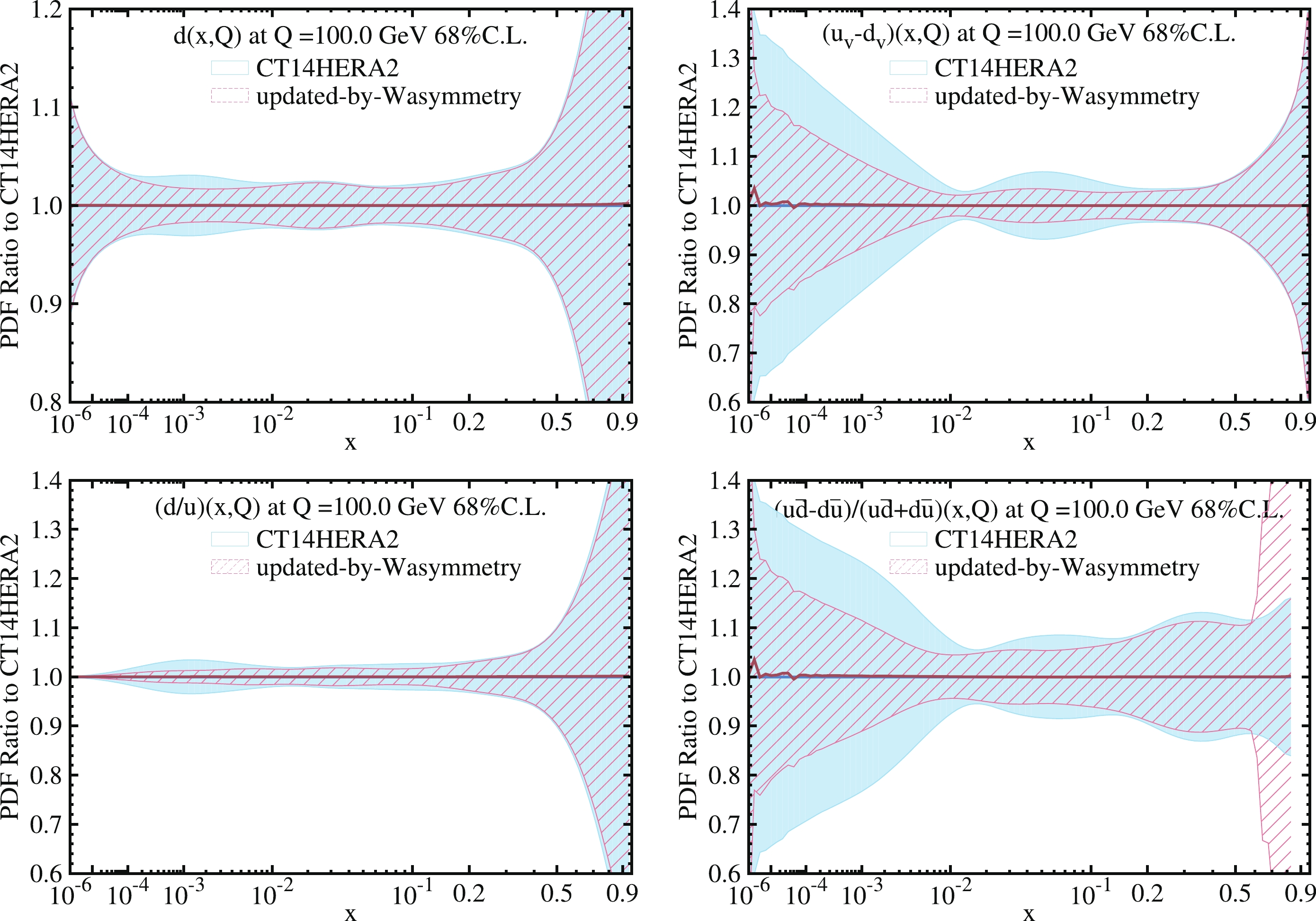
Figure 7. (color online) Ratios of the central value and uncertainty to the CT14HERA2 central value of the d,
$u_v-d_v$ ,$d/u$ and$(u{\bar d}-d{\bar u})/(u{\bar d}+d{\bar u})$ PDFs, before and after the PDF updating. The blue band corresponds to the uncertainty before updating and the red band is after updating. The lepton charge asymmetry$A_\pm(\eta_{\ell})$ data is used in the updating. -
Since the Drell-Yan
$ A_{\rm FB} $ and the lepton charge asymmetry$ A_\pm(\eta_{\ell}) $ provide complementary information, it is expected that the PDF-induced uncertainty in the determination of$ {\sin^2\theta_{{\rm{eff}}}^{\ell}} $ can be further reduced if we use both the sideband$ A_{\rm FB} $ and the$ A_\pm(\eta_{\ell}) $ data together to update the PDFs. The$ {\sin^2\theta_{{\rm{eff}}}^{\ell}} $ value in the W and Z pseudo-data samples generation is set to be 0.2345, although for the W samples, ResBos does not use$ {\sin^2\theta_{{\rm{eff}}}^{\ell}} $ as direct input, and it is thus independent. Applying the same analysis to those two pseudo-data sets, as detailed in the previous sections, we obtain the results listed in Table 11, which should be directly compared to Table 9 for using the sideband$ A_{\rm FB} $ data and Table 10 for using the$ A_\pm(\eta_{\ell}) $ data alone. We find that using both data sets to update the PDFs could further reduce the PDF-induced uncertainty on the$ {\sin^2\theta_{{\rm{eff}}}^{\ell}} $ measurement, which is determined using the$ A_{\rm FB} $ data in the Z-pole mass window, by about 28% as compared to that using only the sideband$ A_{\rm FB} $ data.Update PDF using sideband $A_{\rm FB}$ and

$A_\pm(\eta_{\ell})$ 

Potential bias on $\sin^2 \theta _{{\rm{eff}}}^{\ell} $ 

PDF uncertainty on $\sin^2 \theta _{{\rm{eff}}}^{\ell} $ 

Statistical uncertainty on $\sin^2 \theta _{{\rm{eff}}}^{\ell} $ 

${\rm CC}$ events:

0.00009 0.00032 0.00015 ${\rm CF}$ events:

0.00018 0.00021 0.00007 ${\rm CC+CF}$ events:

0.00010 0.00021 0.00006 Table 11. Bias, PDF-induced uncertainty and statistical uncertainty on
$\sin^2 \theta _{W}$ , after updating the PDFs with the sideband range of the$A_{\rm FB}$ pseudo-data (with$\sin^2 \theta _{W}=0.2345$ ) and the$A_\pm(\eta_{\ell})$ pseudo-data samples, for the${\rm CC}$ and${\rm CF}$ event samples, respectively. The PDF uncertainties are given at 68% C.L. -
To further discuss the improvement in PDF-induced uncertainties, we apply the ePump optimization method of the
$ {\texttt{ePump }}$ code in this section, in the combined analysis of the$ A_{\rm FB} $ and$ A_\pm(\eta_{\ell}) $ data, (1) to demonstrate their complementary roles in reducing the PDF uncertainty in the PDF-updating procedure; and (2) to investigate the optimal choice of bin size for studying the PDF-induced uncertainty in experimental observables related to those two individual data. -
The ePump optimization (or PDF-rediagonalization) method is based on ideas similar to that used in the data set diagonalization method developed by Pumplin [23].
For a set of new data points, the application constructs an equivalent set of eigenvectors, which are orthogonal to each other in the PDF fitting parameter space, by re-diagonalizing the original Hessian error PDFs with respect to the given data. The total uncertainty calculated by the new eigenvectors is exactly identical to that calculated with the original error PDFs in the linear approximation assumed by the Hessian analysis. However, in addition, the new error PDF pairs are ordered by the magnitudes of their re-calculated eigenvalues, the sum of which should be identical to the total number of the given data points, as noted in Ref. [15]. That is to say that the new eigenvectors can be considered as projecting the original error PDFs to the given data set, and be optimized or re-ordered so that it is easy to choose a reduced set that covers the PDF uncertainty for the input data set to any desired accuracy [15].
As an example, after applying the ePump optimization method to the CT14HERA2 PDFs for the sideband
$ A_{FB} $ and$ A_{\pm}(\eta_{\ell}) $ data sets, which contain 50 data points in total (i.e., 25 bins in each case), we find that the top three new eigenvector pairs predominantly have eigenvalues of 25.2, 18.1 and 5.5, respectively, while the eigenvalues of remaining ones decrease rapidly after that. The combination of these top 3 optimized error PDFs contributes up to 97.6% in the total PDF variance of the 50 given data points. This ePump optimization allows us to conveniently use these 3 leading new eigenvectors, in contrast to applying the full 56 error sets of the CT14HERA2, to study the PDF-induced uncertainty on$ A_{\rm FB} $ and$ A_\pm(\eta_{\ell}) $ or any other observable that is directly related to them.The relative contributions of the top three leading optimized eigenvectors to the PDF uncertainties of the sideband
$ A_{\rm FB} $ and$ A_{\pm}(\eta_{\ell}) $ , normalized to each bin for illustration, are shown in Fig. 8. One can see directly that the first eigenvector (labeled as EV01) gives by far the largest contribution to the PDF uncertainties of the sideband$ A_{\rm FB} $ , but a very small fraction of the uncertainties of$ A_{\pm}(\eta_{\ell}) $ , particularly for$ |\eta_{\ell}|>1 $ . The second and third eigenvectors (labeled as EV02 and EV03) contribute a large or appreciable amount of the uncertainties on$ A_{\pm}(\eta_{\ell}) $ , but a much smaller fraction on$ A_{\rm FB} $ . This suggests that when optimizing PDFs using both the$ A_{\rm FB} $ and$ A_{\pm}(\eta_{\ell}) $ samples, these two data sets play complementary roles in reducing the PDF uncertainties, i.e., the re-diagonalization of the first pair of eigenvectors is dominated by the information from the$ A_{\rm FB} $ and the second pair has more information from$ A_{\pm}(\eta_{\ell}) $ .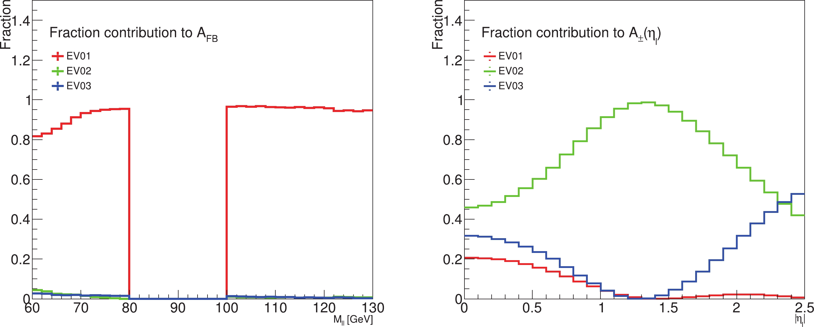
Figure 8. (color online) Fractional contribution of the top three leading optimized eigenvectors (EV01, EV02 and EV03) to the variance of the observables
$A_{\rm FB}$ and$A_\pm(\eta_{\ell})$ , normalized to each bin respectively, in the combined ePump optimization analysis.The sensitivities provided by the top two pairs of eigenvector PDFs to the different flavor and x-range, probed by the sideband
$ A_{\rm FB} $ and the lepton charge asymmetry$ A_{\pm}(\eta_{\ell}) $ together, are depicted in Fig. 9 and Fig. 10, respectively. It can be verified that these two leading pairs of error PDFs, optimized by using both of those two data sets, resemble the respective first pair of eigenvector PDFs after applying the ePump optimization procedure to the sideband$ A_{\rm FB} $ and the$ A_{\pm}(\eta_{\ell}) $ alone. This information can be understood from the following physical argument.$ A_{\rm FB} $ is dependent on PDFs predominantly because the dilution effect could lead to an incorrect assignment of the z direction of the Collins-Soper definition. At the LHC, the leading order dilution probability that forward and backward is misjudged depends only on the relative size of PDF ratios$ u/\bar{u} $ and$ d/\bar{d} $ , meaning that it is more sensitive to the quark-antiquark comparison. For$ A_{\pm}(\eta_{\ell}) $ , this asymmetry comes from the difference between the$ u\bar{d} $ cross section and the$ d\bar{u} $ cross section, meaning that it is more sensitive to the flavor difference. As shown in Fig. 9, the first eigenvector pair, which gives the largest PDF contribution to the$ A_{\rm FB} $ uncertainty, dominates the$ u/\bar{u} $ uncertainty in the x region of a Z boson process. The$ d/\bar{d} $ uncertainty is not as dominated by the first eigenvector, because the Z-quark couplings of neutral vector current, which govern the magnitude of$ A_{\rm FB} $ at parton level, are proportional to the electric charges of different quark types, so that the sensitivity of$ A_{\rm FB} $ to$ d/\bar{d} $ parton distribution is suppressed. Since the observed$ A_{\rm FB} $ is a combination of$ u\bar{u} $ and$ d\bar{d} $ processes, it can provide some information on the difference between u and d quark PDFs, but it is not as sensitive to this as it is to the$ u/\bar{u} $ and$ d/\bar{d} $ ratios. In Fig. 10, the second eigenvector pair, which gives the largest PDF contribution to the$ A_{\pm}(\eta_{\ell}) $ uncertainty, dominates the$ d/u $ and$ \bar{d}/\bar{u} $ uncertainties in the x region of the single W boson process. However, it has almost no sensitivity to the$ \bar{u}/u_{v} $ uncertainty in the very large x-range.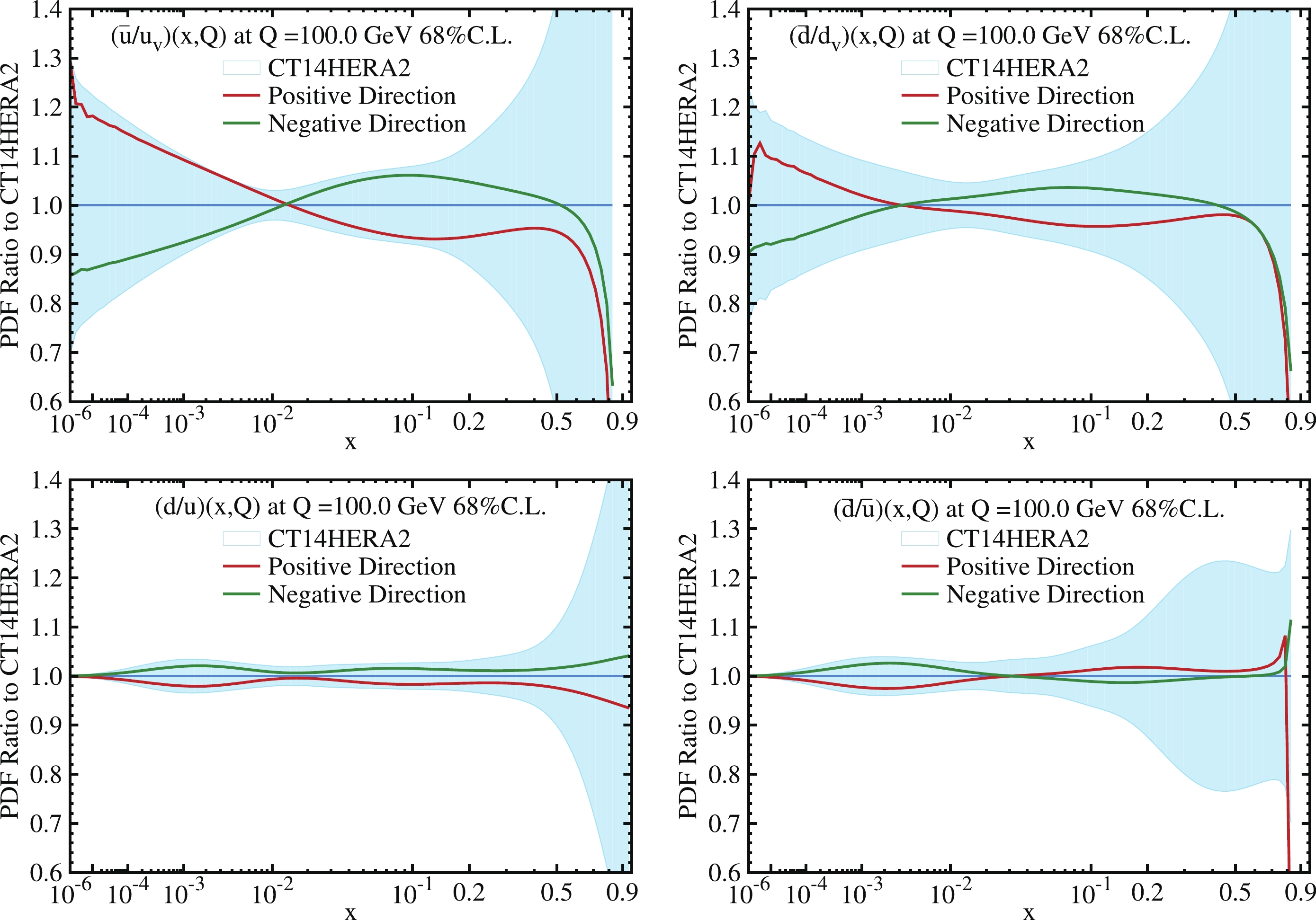
Figure 9. (color online) Ratios of the first pair of eigenvector PDFs and the original CT14HERA2 error PDFs, at
$Q=100$ GeV, to the CT14HERA2 central value of the${\bar u}/{u_v}$ ,${\bar d}/{d_v}$ ,$d/u$ and$\bar d/\bar u$ PDFs. Those eigenvector PDFs were obtained after applying the ePump optimization to the original CT14HERA2 PDFs in the combined analysis of the Drell-Yan sideband$A_{\rm FB}$ and the lepton charge asymmetry$A_\pm(\eta_{\ell})$ data.
Figure 10. (color online) Same as Fig. 9, but for the second pair of eigenvector PDFs.
-
In previous sections, a bin size of 2 GeV on mass was used for measuring the
$ A_{\rm FB} $ distribution, and a bin size of 0.1 on$ \eta_{\ell} $ was used for$ A_\pm(\eta_{\ell}) $ . In principle, using a large bin size will smear some fine structures of the$ A_{\rm FB} $ and$ A_\pm(\eta_{\ell}) $ distributions, and make those observables less sensitive to variations of the PDFs. Hence, it is desirable to determine the maximum allowed bin size without losing sensitivity for a given observable. Due to the difficulty in the experimental unfolding procedure to remove detector effects, such as bin-to-bin migration effects and determination of efficiency and acceptance, it may not always be practical to measure the$ A_{\rm FB} $ and$ A_\pm(\eta_{\ell}) $ distributions in such a fine bin configuration. In this section, we discuss how to apply the ePump optimization procedure to obtain the optimal choice of bin size for$ A_{\rm FB} $ and$ A_\pm(\eta_{\ell}) $ distributions.From Sec. VIA, we learned that the PDF-induced error on
$ A_{\rm FB} $ and$ A_\pm(\eta_{\ell}) $ can be represented by the leading eigenvectors after ePump optimization. In Fig. 11, we show the$ A_{\rm FB} $ distributions, predicted by the first two eigenvector PDF sets, after PDF-rediagonalization. For each eigenvector, positive and negative shifted PDF error sets are compared. Similarly, for the$ A_\pm(\eta_{\ell}) $ distribution, comparisons are shown in Fig. 12.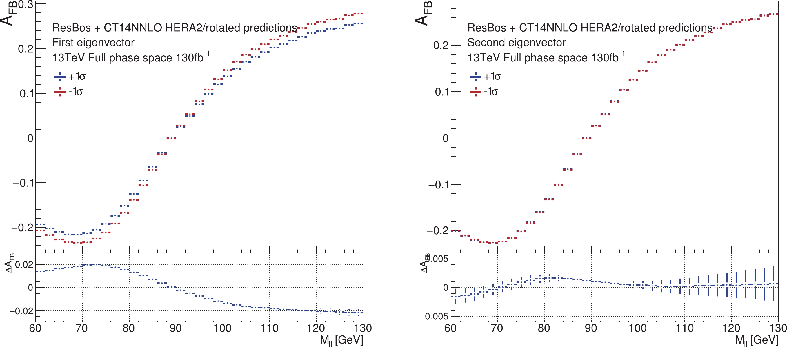
Figure 11. (color online)
$A_{\rm FB}$ distribution predicted by the first and second eigenvector PDF sets, after applying the ePump optimization method to optimize the CT14HERA2 PDFs for the$A_{\rm FB}$ data, as described in the text. Predictions from the positive and negative shifted error sets of each eigenvector PDF set are compared, and$\Delta A_{\rm FB}$ is their difference.
Figure 12. (color online) Similar to Fig. 11, but for
$A_\pm(\eta_{\ell})$ distribution.When the PDFs are varied according to the first pair of eigenvector sets, the most significant change in the shape of the
$ A_{\rm FB} $ distribution occurs as an oppositely shifted effect in the high mass and low mass regions around the Z pole, cf. the left-hand plot of Fig. 11. Moreover, the shape of$ \Delta $ is almost flat either below or above the Z-pole mass window, where$ \Delta $ is the difference between the two values of$ A_{\rm FB} $ predicted by the positive and negative shifted error sets. As a result, using a larger bin size on mass will not lose much information on how the PDFs affect the$ A_{\rm FB} $ distribution. On the other hand, as shown in the right-hand plot of Fig. 12, when the PDFs are varied according to the second pair of eigenvector sets, the change of$ \Delta $ in the shape of$ A_\pm(\eta_{\ell}) $ distribution is almost a linear-type. Hence, as long as the bin size on lepton rapidity still reflects the linear shape, the sensitivity of$ A_\pm(\eta_{\ell}) $ to PDF variations should not be dramatically reduced.To quantitatively study the sensitivity loss from using a larger bin size, we compare with another analysis done by using a bin size of 5 GeV on mass for the
$ A_{\rm FB} $ distribution, and a bin size of 0.25 on lepton$ \eta $ for the$ A_\pm(\eta_{\ell}) $ distribution, for the same data samples as used in Section V. We find that numerical calculations using these wide bins give exactly the same results as those presented in the previous tables, which implies that the reduction of PDF uncertainty would not be compromised by using a larger bin size, as proposed above. This leads to a very useful conclusion: aiming for the$ {\sin^2\theta_{{\rm{eff}}}^{\ell}} $ measurement, both$ A_{\rm FB} $ and$ A_\pm(\eta_{\ell}) $ distributions can be measured in a large bin size to reduce systematic uncertainties without losing much sensitivity in constraining the PDFs. This conclusion should hold for both a quick PDF-updating and a full PDF global fitting. This conclusion is important, because as more data accumulates at the LHC, systematic uncertainties will soon be larger than the statistical uncertainty for many precision measurements. Therefore, reducing systematics should be of a higher priority. -
We have presented a study on how to correctly reduce the PDF-induced uncertainty in the determination of the effective weak mixing angle
$ {\sin^2\theta_{{\rm{eff}}}^{\ell}} $ , obtained from analyzing the measurement of the Drell-Yan forward-backward asymmetry$ A_{\rm FB} $ at the LHC. According to previous studies, the PDF-induced uncertainty can be reduced by the PDF updating procedure using$ A_{\rm FB} $ . However, when$ A_{\rm FB} $ is used for both PDF updating and$ {\sin^2\theta_{{\rm{eff}}}^{\ell}} $ extraction, the correlation between these two important tasks will cause bias on both the updated PDFs and the extracted value of$ {\sin^2\theta_{{\rm{eff}}}^{\ell}} $ . Considering the deviation between the previous precise measurements on$ {\sin^2\theta_{{\rm{eff}}}^{\ell}} $ , such bias could be at the same level as the PDF-induced uncertainty on$ {\sin^2\theta_{{\rm{eff}}}^{\ell}} $ . In this paper we have shown how this bias can be suppressed.$ A_{\rm FB} $ is more sensitive to$ {\sin^2\theta_{{\rm{eff}}}^{\ell}} $ around the Z pole, while the PDFs affect$ A_{\rm FB} $ more significantly in the sideband regions such as$ 60 < M_{ll}<80 $ GeV and$ 100 < M_{ll}<130 $ GeV. Accordingly, we propose to use the sideband$ A_{\rm FB} $ to reduce the correlation between the$ {\sin^2\theta_{{\rm{eff}}}^{\ell}} $ extraction and the PDF updating, so that the bias on the$ {\sin^2\theta_{{\rm{eff}}}^{\ell}} $ determination can be suppressed, while not significantly losing sensitivity in the PDF updating.We have applied the
$ {\texttt{ePump }}$ program, based on the Hessian updating method, to update the CT14HERA2 PDFs by including the full mass range$ A_{\rm FB} $ pseudo-data as new input to a global PDF fitting. With this updated PDF set, we analyzed the extraction of$ {\sin^2\theta_{{\rm{eff}}}^{\ell}} $ in the Z-pole mass window and found a sizable bias in its value, with respect to its input value in the pseudo-data. Furthermore, the central values of the updated d and u quark PDFs, obtained from this analysis, are different from those of the original CT14HERA2 PDFs. This is caused by the difference in the$ {\sin^2\theta_{{\rm{eff}}}^{\ell}} $ values assumed in the pseudo-data and the theory templates. To reduce this type of correlation, we proposed to use only the sideband$ A_{\rm FB} $ to update the existing PDFs. As expected, using only the sideband$ A_{\rm FB} $ data to update the PDFs reduces the bias on the extraction of$ {\sin^2\theta_{{\rm{eff}}}^{\ell}} $ value as well as the central values of the updated PDFs. We also show that the asymmetry from W boson decay,$ A_\pm(\eta_{\ell}) $ , can be used to further reduce the PDF uncertainty. It plays a complementary role to the sideband$ A_{\rm FB} $ data in reducing the PDF-induced uncertainty, with negligible bias on the determination of the weak mixing angle.A study on the effect of choosing different bin sizes of the
$ A_{\rm FB} $ and$ A_\pm(\eta_{\ell}) $ distributions was also performed. It showed that using a somewhat larger bin size will not sacrifice much of the sensitivity of those two observables in reducing the PDF uncertainty in the$ {\sin^2\theta_{{\rm{eff}}}^{\ell}} $ measurement. When more data are accumulated at the LHC, the systematic uncertainties in the$ A_{\rm FB} $ and$ A_\pm(\eta_{\ell}) $ measurements will begin to dominate. In that case, there is an advantage in choosing a larger bin size in order to reduce the systematic uncertainties in the experimental unfolding procedures. In this study, using a bin size of 5 GeV on mass for the$ A_{\rm FB} $ distribution, and a bin size of 0.25 on lepton$ \eta $ for the$ A_\pm(\eta_{\ell}) $ distribution, did not cause a noticeable reduction in the sensitivity of these two data sets to the measurement of$ {\sin^2\theta_{{\rm{eff}}}^{\ell}} $ .In conclusion, we have investigated the correlation and potential bias in reducing the PDF-induced uncertainty in the determination of
$ {\sin^2\theta_{{\rm{eff}}}^{\ell}} $ from the forward and backward asymmetry$ A_{\rm FB} $ of the Drell-Yan processes at the LHC. Derived from quantitative computation of the Hessian-based$ {\texttt{ePump }}$ PDF updating program, it can be concluded that by excluding Z-pole region events in the PDF updating, the potential bias on the$ {\sin^2\theta_{{\rm{eff}}}^{\ell}} $ extraction would not significantly enlarge the estimated total uncertainty, including the statistical and PDF-induced uncertainties at the LHC Run 2. However, the bias is not negligible and thus still needs careful evaluation in future precise$ {\sin^2\theta_{{\rm{eff}}}^{\ell}} $ measurements at the high luminosity LHC. Moreover, although it is useful to quickly use$ {\texttt{ePump }}$ to estimate the impact of a new data set on the PDFs, we suggest using the PDF updating method as only a preliminary way to reduce the PDF-induced uncertainty in the$ {\sin^2\theta_{{\rm{eff}}}^{\ell}} $ measurements. A full PDF global fitting analysis is necessary for a complete determination of$ {\sin^2\theta_{{\rm{eff}}}^{\ell}} $ with PDF correlations, in which new degrees of freedom in the non-perturbative parametrization of the PDFs can be explored. Furthermore, all experimental results, i.e.,$ A_{\rm FB} $ and$ A_\pm(\eta_{\ell}) $ studied in this article, should be provided in a format such that theorists can replace the preliminary PDF updating method employed in the experimental analysis by a consistent global analysis. -
C.-P. Yuan is grateful for support from the Wu-Ki Tung Endowed Chair in Particle Physics.
-
Consider that if the directions of the initial state quarks and antiquarks in the DY events are known, one can define a Collin-Soper frame at hadron colliders without any dilution effect. In this situation, the differential cross section of the DY process can be written as:
$\tag{A1}\begin{aligned}[b]& \frac{{\rm d}\sigma_q}{{\rm d}\cos\theta^*_q} \sim (1+\cos^2\theta^*_q) + A^q_0 \\&\quad\times \frac{1}{2}(1-3\cos^2\theta^*_q) + A^q_4 \times \cos\theta^*_q, \end{aligned} $

where the label q is used to mark the no-dilution cross section at partonic level. In reality, the dilution effect can lead to an incorrect assignment of the z direction in the Collins-Soper frame, resulting in:
$\tag{A2} \cos\theta^*_h = \cos(\pi - \theta^*_q) = -\cos\theta^*_q, $

where the label h is used to mark the dilution case at hadronic level. With a dilution probability of f, we have:
$ \begin{aligned}[b] \frac{{\rm d}\sigma_h}{{\rm d}\cos\theta^*_h} =& f \times \frac{{\rm d}\sigma_q}{{\rm d}\cos\theta^*_q}\Big|_{\cos\theta^*_q = -\cos\theta^*_h} \\&+ (1-f) \times \frac{{\rm d}\sigma_q}{{\rm d}\cos\theta^*_q}\Big|_{\cos\theta^*_q = \cos\theta^*_h} \\&\sim (1+\cos^2\theta^*_h) + A^q_0 \times \frac{1}{2}(1-3\cos^2\theta^*_h) \end{aligned}$

$\tag{A3} \begin{aligned}[b] + (1-2f) \times A^q_4 \times \cos\theta^*_h. \end{aligned}$

Accordingly,
$\tag{A4} A^h_4. = (1-2f)A^q_4 $

Since the
$ A_{\rm FB} $ around the Z pole is proportional to the angular coefficient$ A_4 $ , it turns out that$\tag{A5} A^h_{\rm FB} = (1-2f) A^q_{\rm FB} $

The sensitivity of constraining the PDFs (namely constraining f) via
$ A_{\rm FB} $ depends on the$ A_{\rm FB} $ value itself.
Reduction of PDF uncertainty in the measurement of the weak mixing angle at the ATLAS experiment
- Received Date: 2020-08-14
- Available Online: 2021-05-15
Abstract: We investigate the parton distribution function (PDF) uncertainty in the measurement of the effective weak mixing angle


 DownLoad: