


 Abstract
 HTML
HTML Reference
 Related
 PDF
PDF


-
In general relativity, the event horizon of a black hole is defined as the frontier of a region of space-time, where gravity is so strong that nothing, not even light, that enters that region can ever escape. The characteristic features of black holes, including event horizons, accretion and outflow processes, singularities, and Hawking radiation, as well as the possibility of observation of their immediate environment with angular resolution comparable to the event horizon, using facilities such as the Event Horizon Telescope [1] and the GRAVITY instrument [2], make black holes useful laboratories to test general relativity in the strong field regime and, hopefully, to test ideas for quantum gravity.
The accretion process onto compact objects is relevant as it is believed to provide the energy of Quasars, accreting supermassive black holes, X-ray binaries, and Gamma-ray bursts. The simplest situation, which has reached a paradigmatic status in studies on accretion astrophysics, is spherically symmetric accretion onto a static compact object of an inviscid gas, which is at rest at infinity. In the framework of Newtonian gravity the problem was analyzed in a seminal paper by Bondi [3]. The relativistic generalization of the Bondi accretion problem was performed in [4], which was followed by numerous studies analyzing spherical accretion onto a wide variety of astrophysical objects, including black holes [5-18].
The problem of the stability of spherically symmetric accretion under linearized perturbations has been studied extensively in the literature both in the context of Newtonian gravity [19-22] and in the classical general relativistic realm [23-31]. In both of these regimes, no evidence has been found of the development of instabilities. In [19], it has been shown that in the Newtonian regime and neglecting viscosity, the perturbation has a constant amplitude for the conserved flow so that stability is ensured. In general relativity, the background solution is likewise stable with the amplitude of the perturbation being damped in time, that is, general relativistic effects enhance the stability [23, 30, 31]. A mechanism that favors stability in this case is the coupling of the infalling flow with the geometry of space-time, which acts in the manner of a dissipative effect.
In this work, we consider quantum gravity corrections to the accretion, and to its stability, onto an improved Schwarzschild black hole in the framework of the asymptotic safety scenario for quantum gravity. In this scenario, it is conjectured that gravity constitutes a fundamental theory at the non-perturbative level [32]. A basic ingredient in this construction is a non-Gaussian fixed point (NGFP) of the gravitational renormalization group (RG) flow, which controls the behavior of the theory at trans-Planckian energies, where the physical degrees of freedom interact predominantly antiscreening, which in turn renders physical quantities safe from unphysical divergences at all scales [33]. This means that the gravitational field itself is the principal carrier of relevant classical and quantum degrees of freedom, with the renormalization flow relating its infrared and ultraviolet physics. On the condition that the set of RG trajectories approaching the fixed point in the UV are parameterized by a finite number of relevant (i.e., physically motivated) running couplings, asymptotic safety is as predictive as the standard perturbatively renormalizable quantum field theory. Notwithstanding asymptotic safety defines a consistent and predictive quantum theory for gravity within the framework of quantum field theory, it remains a prediction in the sense that a rigorous existence proof for the NGFP is still lacking. There is, however, substantial evidence for the existence of such a fixed point suitable for the Weinberg's asymptotic safety scenario [34-50].
Quantum corrections to the structure of black hole spacetimes within the asymptotic safety program was initiated in [51] by constructing the so-called "RG-improved" solution to the Schwarzschild metric. Following up on these initial studies, the RG-improved Kerr metric has been discussed in [52], and the improved Schwarzschild-(A)dS and Reissner-Nordström-(A)dS metrics have been studied in [53] and [54], respectively. The inclusion of a cosmological constant is relevant, as it has been shown in [53] that this constant determines the short-distance structure of the RG-improved black holes. Further aspects of these quantum compact objects including thermodynamical properties, evaporation processes, and mini-black hole production, have been analyzed in [55-59], while quantum corrections to the accretion process onto a Schwarzschild black hole have been discussed in [60, 61].
In this paper, we review the results reported by the authors of [61], where the study of the accretion onto an improved asymptotically safe Schwarzschild metric with high-derivative terms was conducted; we furrther discuss the stability of the accretion process and contrast it with the result from GR. The interest in the improved Schwarzschild space-time with higher-derivatives in the infrared limit arises from the fact that, as shown in [62], it describes a black hole that never completely evaporates. Consequently, it makes an excellent dark matter candidate. Because our interest is to analyze the most general aspects of the problem, we will neglect viscous effects, heat transport, fluid self-gravity, and effects associated to the back-reaction of the fluid on the geometry. As done in [61], we describe the accretion process of isothermal fluids using the Hamiltonian dynamical formalism and show that, contrary to what claimed in that work, there are physical solutions for the accretion of an ultra-relavitivistic fluid in AS. Regarding the analysis of the stability, instead of adopting the approach of perturbing a scalar potential whose gradient is prescribed to be the velocity of the ideal fluid [23], we use a perturbation scheme based on the continuity equation [19, 20, 30, 31]. The stationary solution of the continuity equation gives a first integral, which within a constant geometric factor, is the matter accretion rate. Our perturbative procedure entails the perturbation of this constant of motion. This quantity, being a flux of mass can be observed and, in principle, can be measured using the present day and the projected observational instruments [1, 2].
This paper is organized as follows. In the next section, we present the RG-improved Schwarzschild metric. In Sec. III, we review the mathematics of the accretion process and present the Hamiltonian dynamical system formalism. In Sec. IV, we apply the formalism to the spherically symmetric accretion of isothermal fluids and analyze the quantum gravity effects by comparing with the GR description. In Sec. V, we discuss the implementation of the perturbation scheme based on the continuity equation, and analyze the quantum gravity corrections to the stability of the accretion by studying the behavior of standing wave and traveling wave perturbations to the mass accretion rate. Finally, in the last section, we present our conclusions.
-
We start by recalling that the classical Schwarzschild line element for a black hole with mass
$ M $ , in units$ c = G_{0} = 1 $ , is written as$ {\rm d}s^2 = -f_0(r){\rm d}t^2+f_0(r)^{-1}{\rm d}r^2+r^2\Big({\rm d}\theta^2+\sin^2\theta {\rm d}\varphi^2\Big), $

(1) with the metric coefficient
$ g^{tt} $ given by:$ f_0(r) = 1-2M/r $ . The event horizon or Schwarzschild radius comes from solving$ f_0(r) = 0 $ , which yields$r_{\rm hS} = 2M$ .In the high-derivative gravity theory, which includes the Ricci scalar square, the Ricci tensor square, the Kretschmann scalar, and running gravitational couplings in the effective action [62], the quantum gravity corrections to the metric are accounted for by promoting the classical gravitational Newton constant through a running coupling that evolves under the equations of the gravitational RG-flow. Thus, in the low energy limit the RG-improvement to the metric in Eq. (1) is obtained by doing
$ f_0(r) \rightarrow f(r) = 1-\frac{2M}{r}\left(1-\frac{\xi}{r^2}\right), $

(2) where
$ \xi $ is a parameter with dimensions of length squared associated to the scale identification between the momentum scale$ p $ and the radial coordinate$ r $ , which in the IR regime, takes the form$ p \sim 1/r $ . Notably, the quantum effects on the space-time geometry are all encoded in$ \xi $ , such that for$ \xi = 0 $ the classical metric coefficient$ f_0(r) $ is recovered. The condition for the radius of the new event horizon:$ f(r) = 0 $ , takes the form of a generic cubic equation$ r^3-2 M r^2+2 M^3 \tilde{\xi} = 0, $

(3) where the dimensionless parameter
$ \tilde{\xi} = \xi/M^2 $ has been introduced for convenience. The only real solution$r_{\rm hIR}$ to Eq. (3) is$ \begin{aligned}[b] \frac{r_{\rm hIR}}{r_{\rm hS}} =& \frac{1}{6} \left(2+\frac{4}{\sqrt[3]{8-27 \tilde{\xi} +3 \sqrt{3} \sqrt{\tilde{\xi} (27 \tilde{\xi} -16)}}}\right.\\&\left.+\sqrt[3]{8-27 \tilde{\xi} +3 \sqrt{3} \sqrt{\tilde{\xi} (27 \tilde{\xi} -16)}}\right). \end{aligned}$

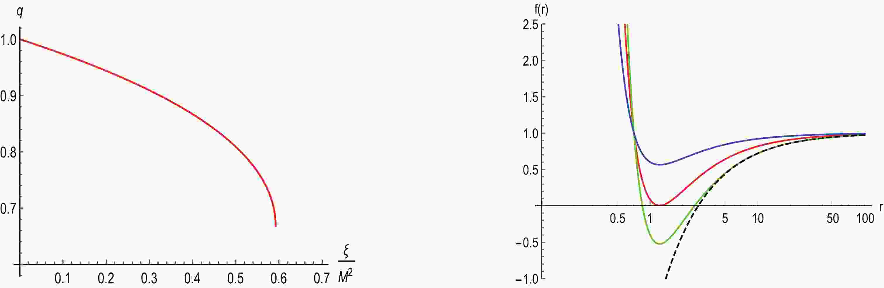
(4) The left panel in Fig. 1 shows the quotient
$q\equiv r_{\rm hIR}/r_{\rm hS}$ as a function of$ \tilde{\xi} $ . For$ \tilde{\xi} = 0 $ , we have$r_{\rm hIR} = r_{\rm hS}$ as expected, while for$ \tilde{\xi} $ greater than the critical value$ \tilde{\xi}_{c} = 16/27 $ , there is no horizon at all, and a naked singularity arises. This implies that each value of$ \tilde{\xi} $ in the range$ 0 \leqslant \tilde{\xi} \leqslant \tilde{\xi}_{c} $ selects a critical mass$ M_{c} = \sqrt{27\xi/16} $ in such a way that for$ M>M_{c} $ there are two horizons: one inner Cauchy horizon and one outer event horizon, for$ M<M_{c} $ a naked singularity develops, while when$ M = M_{c} $ the two horizons merge. The right panel in Fig. 1 illustrates this situation for$ \xi = 0.5 $ that is, for$ M_c = 0.918 $ . Because our aim is to discuss quantum gravity effects on the accretion onto a Schwarzschild black hole, naked space-time singularities will be ignored.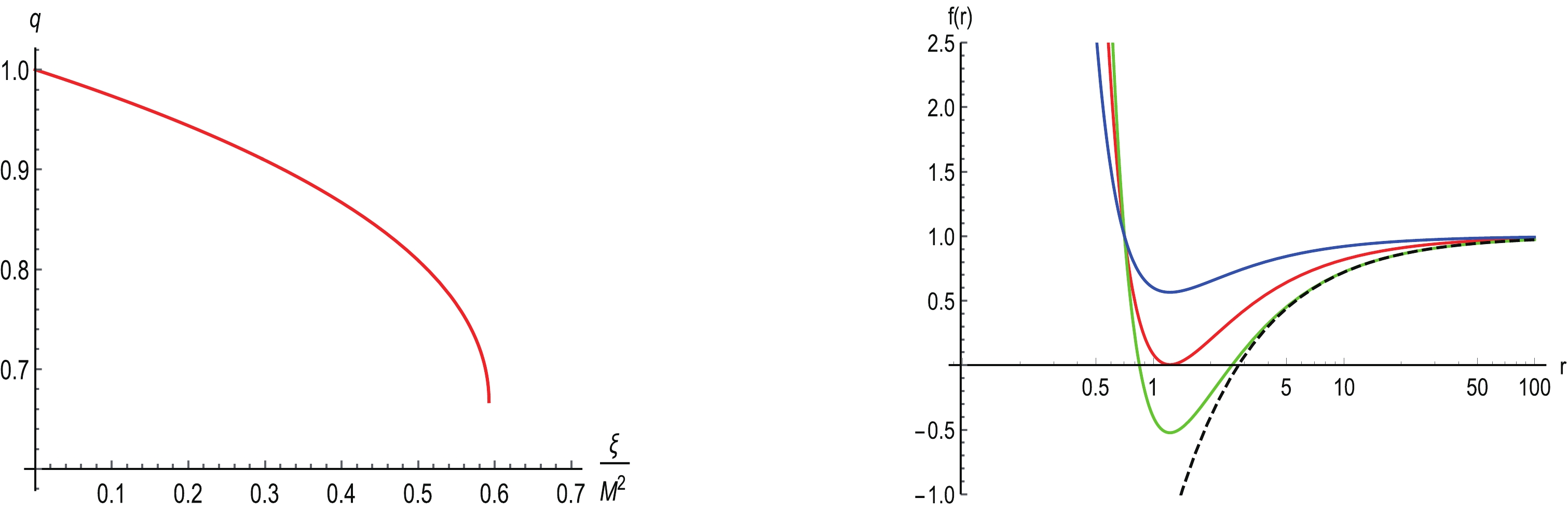
Figure 1. (color online) Left panel: Dependence of
$q\equiv r_{\rm hIR}/r_{\rm hS}$ on$ \tilde{\xi} = \xi/M^2 $ . Rigt panel: plots of the improved metric coefficient$ f(r) $ for$ M<M_{c} $ (blue),$ M = M_{c} $ (red), and$ M>M_{c} $ (green), with$ M_{c} = 0.918 $ corresponding to$ \xi = 0.5 $ . The dashed line correspond to the classical$ f_0(r) $ for$ M = M_{c} $ .For future reference, we note that for
$ M>M_{\mathrm{c}} $ , the outer horizon of the improved solution, upon expanding to the leading order in$ \xi $ , acquires the form:$r_{\rm hIR} = $ $ r_{\rm hS}-\xi /(2M)$ . This result exhibits the typical shifting of the horizon of RG-improved black hole solutions towards smaller values with respect to its classical counterpart. -
Here, we describe the accretion flow by adopting the Hamiltonian procedure. The formulation of the problem of accretion onto compact objects as a Hamiltonian dynamical system was proposed for the first time in [63-65].
We first recall that the phenomenon of accretion is based on two conservation laws: the continuity equation, which expresses the conservation of the particle number, and the energy-momentum conservation. These requirements are given, respectively, by the covariant derivatives
$ \begin{array}{l} \nabla_{\mu} \left(\eta u^{\mu} \right) = 0 \qquad \rm{and} \qquad \nabla_{\mu} T^{\mu \nu} = 0, \end{array}$

(5) where
$ \eta $ is the particle number density of the fluid, and$ u^{\mu} $ is the four-velocity of the fluid normalized as$ u^{\mu}u_{\mu} = -1 $ .By omitting effects related to viscosity or heat transport and assuming that the fluid's energy density is sufficiently small, such that its self-gravity can be ignored, the accreting matter can be approximated as a perfect fluid described by the energy-momentum tensor
$ \begin{array}{l} T_{\mu \nu} = \left( \epsilon + p \right) u_{\mu} u_{\nu} + pg_{\mu \nu}, \end{array}$

(6) where
$ \epsilon $ and$ p $ are the proper energy density and the proper pressure of the fluid, respectively.For purely radial flow in the equatorial plane, the normalization condition
$ u^{\mu}u_{\mu} = -1 $ produces$ \begin{array}{l} u_t = -f u^t = \sqrt{f+(u^r)^2} \end{array}$

(7) where
$ u^r $ denotes the radial flow velocity, and$ f = f(r) $ is the metric coefficient in the spherically symmetric line element.We assume as infalling matter a test fluid, which is both isothermal and isentropic, that is a test fluid with a barotropic equation of state
$ h = h(\eta) $ , where$ h $ is the specific enthalpy$ h = \frac{\epsilon + p}{\eta}. $

(8) This fluid is described by the thermodynamical equations
$ \begin{array}{l} {\rm d}p = \eta {\rm d}h, \qquad {\rm d}\epsilon = h{\rm d}\eta, \end{array} $

(9) such that the square of the local speed of sound is written as
$ a^{2} = \frac{\partial p}{\partial \epsilon}\Bigg\vert_{{\rm d}s = 0} = \frac{{\rm d}p}{{\rm d}\epsilon} = \frac{\eta}{h}\frac{{\rm d}h}{{\rm d}\eta} = \frac{{\rm d} \ln h}{{\rm d} \ln \eta}. $

(10) Then, as it is well known, for the spherically symmetric stationary accretion ,the conservation laws in Eq. (3) yield
$ \begin{array}{l} \eta u^r r^2 = C_1, \end{array}$

(11) and
$ \begin{array}{l} h u_t = C_2, \end{array}$

(12) where
$ C_1 $ and$ C_2 $ are arbitrary integration constants.To describe the accretion process as a two-dimensional Hamiltonian dynamical system, it is useful to define the three-velocity
$ v $ of a fluid element as measured by a locally static observer as$v = {\rm d}l/{\rm d}\tau$ , where${\rm d}l = {\rm d}r/\sqrt{f}$ and${\rm d}\tau = \sqrt{f} {\rm d}t$ are the proper radial distance and the proper time, respectively. It is important to remark that$ v $ is defined outside the horizon, that is for an observer for whom the time coordinate is timelike [63-65]. Using$u^r = {\rm d}r/{\rm d}\tau$ ,$u^t = {\rm d}t/{\rm d}\tau$ and Eq. (7) we obtain$ v^2 = \frac{(u^r)^2}{f+(u^r)^2} = \frac{(u^r)^2}{(u_t)^2}, $

(13) from which
$ (u^r)^2 = \frac{fv^2}{1-v^2}, \quad \mathrm{and} \quad (u_t)^2 = \frac{f}{1-v^2}. $

(14) As the Hamiltonian for the flow fluid, we can choose either of the two integrals of motion
$ C_1, C_2 $ , or even any combination of them. We choose$ C_2^2 $ as our Hamiltonian$ H $ and fix the dynamical variables of the system to be$ r $ and$ v $ . Using Eq. (14), we then have$ H(r,v) = \frac{h^2(r,v)f(r)}{1-v^2}, $

(15) and the dynamical system is defined by
$ \dot{r} = \frac{\partial H}{\partial v}, \qquad \dot{v} = -\frac{\partial H}{\partial r}, $

(16) where the dot denotes time derivative. After employing Eq. (10), these two equations become
$ \dot{r} = \frac{2 f h^2}{v(1-v^2)^2}(v^2-a^2), $

(17) $ \dot{v} = -\frac{h^2}{r(1-v^2)}\left[(1-a^2)r \frac{{\rm d}f}{{\rm d}r}-4 f a^2\right]. $

(18) The critical points of the dynamical system, which coincides with the sonic points of the fluid flow, are the points
$ (r_c,v_c) $ , where both$ \dot{r} $ and$ \dot{v} $ are zero. Assuming that$ h\neq 0 $ for all values of$ r>r_{hIR} $ where also$ f\neq 0 $ , it follows that at the critical points$ \begin{array}{l} v_c^2 = a_c^2, \qquad r_c(1-a_c^2)f_{c,r_c} = 4f_c a_c^2, \end{array}$

(19) where
$ f_c = f(r)\vert_{r_c} $ and$f_{c,r_c} = ({\rm d}f/{\rm d}r)\vert_{r_c}$ . -
In this section, according to [66, 67], we will obtain an adequate expression for
$ h(r,v) $ in Eq. (15) when the accreted fluid is isothermal. This in turn provides a neat expression for the Hamiltonian$ H(r,v) $ .The barotropic equation of state for an isentropic fluid can be expressed as
$ \epsilon = \epsilon(\eta) $ . Moreover, for an isothermal fluid, the equation of state reads$ p = k\epsilon $ , where the constant$ k $ is the parameter state:$ 0<k<1 $ . Note that the definition of the speed of sound in Eq. (10) leads to$ a^2 = k $ , and so the speed of sound remains constant through the accretion process. Now, from Eqs. (9) we have$ h = \frac{{\rm d}\epsilon}{{\rm d}\eta}, $

(20) and
$ \frac{{\rm d}p}{{\rm d}\eta} = \eta \frac{{\rm d}h}{{\rm d}\eta} = \frac{{\rm d}^2\epsilon}{{\rm d}\eta^2}, $

(21) which, upon integration, produces
$ \eta \frac{{\rm d}\epsilon}{{\rm d}\eta}-\epsilon(\eta) = k\epsilon(\eta), $

(22) where we used
$ p(\eta) = k\epsilon(\eta) $ . Integration of this last equation yields$ \epsilon(\eta) = C \eta^{k+1} = \frac{\epsilon_c}{\eta_c^{k+1}}\eta^{k+1}, $

(23) where the integration constant
$ C $ has been chosen such that Eqs. (8) and (20) give rise to the same expression for$ h $ $ h(r,\eta) = \frac{(k+1)\epsilon_c}{\eta_c}\left(\frac{\eta}{\eta_c} \right)^k, $

(24) An expression for
$ \eta/\eta_c $ can be obtained from the constant of integration$ C_1 $ in Eq. (11). In fact, using Eqs. (14) and (19), we can write$ C_1^2 = \frac{r^4 \eta^2 f v^2}{1-v^2} = \frac{r_c^4 \eta_c^2 f_c v_c^2}{1-v_c^2} = \frac{r_c^5 \eta_c^2 f_{c,r_c}}{4}, $

(25) such that
$ \left(\frac{\eta}{\eta_c} \right)^k = \left(\frac{r_c^5 f_{c,r_c}}{4}\frac{1-v^2}{r^4 f v^2} \right)^{k/2}. $

(26) Substituting this into Eq. (24), we obtain
$ h^2 = K \left(\frac{1-v^2}{r^4 f v^2}\right)^k, $

(27) with the constant
$ K $ given by$ K = (r_c^5 f_{c,r_c}/4)^k [(k+1)\epsilon_c/\eta_c]^2 $ .Redefining the Hamiltonian as
$ {\cal{H}} = H/K $ and using Eq. (26),$ {\cal{H}} $ finally acquires the form$ {\cal{H}}(r,v) = \frac{[f(r)]^{1-k}}{r^{4k}v^{2k}(1-v^{2})^{1-k}}. $

(28) It must be stressed that, due to the definition of the three-velocity
$ v $ , this expression for$ {\cal{H}} $ is valid for an observer outside the horizon. This applies both for the classical Schwarzschild metric and for the improved AS metric.We now focus on four types of isothermal accretion: ultra-stiff fluid (
$ k = 1 $ ), ultra-relativistic fluid ($ k = 1/2 $ ), radiation fluid ($ k = 1/3 $ ), and sub-relativistic fluid ($ k = 1/4 $ ). For the purpose of comparison with the analysis in [61], we will take$ \xi = 0.5 $ and$ M = 1>M_{c} = 0.918 $ in the expressions for the quantum${\cal{H}}^{\rm (AS)}$ and the classical${\cal{H}}^{\rm(GR)}$ Hamiltonians. Even though this amounts to consider a black hole solution with two horizons, the quantum effects on the accretion we will describe below are present for all values of the parameter$ \xi $ in the range$ 0\leqslant \xi \leqslant (16/27)M^2 $ , with the orbits in the contour plot of the quantum Hamiltonian going continuously towards the orbits of its classical counterpart in the limit$ \xi \rightarrow 0 $ , as we will show ahead. -
The equation of state for ultra-stiff fluid reads
$ p = \epsilon $ , which implies$ a^2 = 1 = v_c^2 $ . Eq. (19) immediately yields$ f_c = 0 $ , and the Hamiltonian in AS coincides with the one in GR$ {\cal{H}}^{\rm (AS)} = {\cal{H}}^{\rm (GR)} = \frac{1}{r^{4}v^{2}}, $

(29) with the only difference being in the location of the horizon that, in both cases, coincides with the location of the critical point:
$r_c^{\rm (AS)} = r_{\rm hIR}$ and$r_c^{\rm (GR)} = r_{\rm hS}$ .Contour plots of
${\cal{H}}^{\rm (AS)}$ (continuous lines) and of${\cal{H}}^{\rm (GR)}$ (dashed line) are shown in Fig. 2, where we have only included selected orbits associated to physical flow ($ \vert v \vert <1 $ ). Here, we retrieve the findings in [61] concerning the contour lines for${\cal{H}}^{\rm (AS)}$ . Notably, both for infalling matter ($ -1<v<0 $ ) and for fluid outflow ($ 0<v<1 $ ), and for fixed values of the radial coordinate$ r $ with$r > r_{\rm hS}$ , the flow velocity is consistently larger in GR than in AS.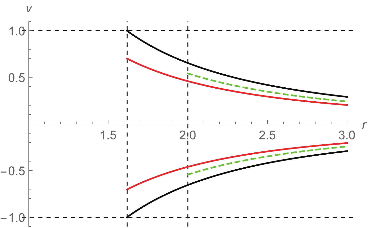
Figure 2. (color online) Contour lines of
${\cal{H}}^{\rm (AS)} = {\cal{H}}_{c}^{\rm (AS)}$ (black) and${\cal{H}}^{\rm (AS)} = {\cal{H}}_{c}^{\rm (AS)}\pm 0.06$ (red) for accretion of ultra-stiff fluid ($ k = 1 $ ). The green dashed curve is the contour line of${\cal{H}}^{\rm (GR)} = {\cal{H}}_{c}^{\rm (GR)}\pm 0.06$ .${\cal{H}}_{c}^{\rm (AS,GR)}$ stands for${\cal{H}}^{\rm (AS,GR)}(r)\vert_{r_c}$ . For all the orbits:$ M = 1 $ ,$ \xi = 0.5 $ . The vertical dashed lines locate the horizons$r_{\rm hIR}$ (left) and$r_{\rm hS}$ (right). The horizontal dashed lines locate the speed of sound$ a = \sqrt{k} $ .We note that we have restricted the comparison between classical and quantum accretion and outflow to the region
$r > r_{\rm hS}$ in the plots, because this is the region for which the comparison makes sense. -
In the case of an ultra-relativistic fluid we have
$ a^2 = 1/2 = v_c^2 $ , and the Hamiltonians reads$ {\cal{H}}^{\rm (AS)} = \frac{\sqrt{1-\dfrac{2M}{r}+\dfrac{2M\xi}{r^3}}}{r^{2}v\sqrt{1-v^{2}}}, \quad {\cal{H}}^{\rm (GR)} = \frac{\sqrt{1-\dfrac{2M}{r}}}{r^{2}v\sqrt{1-v^{2}}}. $

(30) For the critical radii, we obtain
$\begin{aligned}[b] r_c^{\rm (AS)}\simeq \frac{5}{2} M - \frac{14}{25}\frac{\xi}{M}, \quad r_c^{\rm (GR)} = \frac{5}{2}M, \end{aligned}$

(31) where
$r_c^{\rm (AS)}$ is given at leading order in$ \xi $ .In Fig. 3, the contour plots of
${\cal{H}}^{\rm (AS)}$ (continuous lines) and of${\cal{H}}^{\rm (GR)}$ (dashed line) are shown. For readability of the figure, we have not depicted the contour line${\cal{H}}^{\rm (GR)} = {\cal{H}}_{c}^{\rm (GR)}$ . The important fact here is the existence of orbits associated to physical flow ($ \vert v \vert <1 $ ) in AS, which includes the subsonic regime ($ -v_c<v<v_c $ ), supersonic regime ($ -v<-v_c $ and$ v>v_c $ ), and transonic regime associated to the solution passing through the sonic point. This is the opposite to the findings by the authors in [61], where no physical significance was established for accretion of an ultra-relativistic fluid in AS. Two quantum gravity effects can be identified: a shifting of the orbits towards the black hole and an increase of the maximum flow velocity, which occurs at$ r = r_c $ , as compared with the case in GR.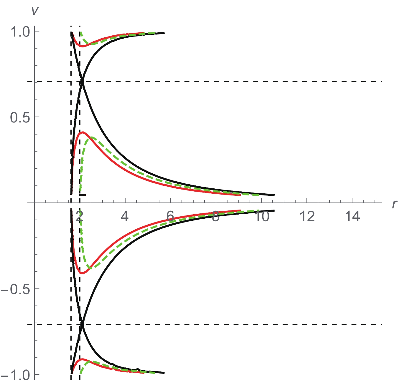
Figure 3. (color online) Contour lines of
${\cal{H}}^{\rm (AS)} = {\cal{H}}_{c}^{\rm (AS)}$ (black) and${\cal{H}}^{\rm (AS)} = {\cal{H}}_{c}^{\rm (AS)}\pm 0.06$ (red) for accretion of ultra-relativistic fluid:$ k = 1/2 $ . The green dashed curve is the contour line of${\cal{H}}^{\rm (GR)} = {\cal{H}}_{c}^{\rm (GR)}\pm 0.06$ . For all the orbits:$ M = 1 $ ,$ \xi = 0.5 $ . The vertical dashed lines locate the horizons$r_{\rm hIR}$ (left) and$r_{\rm hS}$ (right). The horizontal dashed lines locate the speed of sound$ a = \sqrt{k} $ . -
For a radiation fluid, the critical radii are given by
$ r_c^{\rm (AS)} \simeq 3 M-\frac{5}{9}\frac{\xi}{M}, \qquad r_c^{\rm (GR)} = 3 M, $

(32) while the AS and RG Hamiltonians takes respectively the form
$ \begin{aligned}[b] {\cal{H}}^{\rm (AS)} =& \frac{\Bigg(1-\dfrac{2M}{r}+\dfrac{2M\xi}{r^3}\Bigg)^{2/3}}{r^{4/3}v^{2/3}(1-v^{2})^{2/3}}, \\ {\cal{H}}^{\rm (GR)} =& \frac{\Bigg(1-\dfrac{2M}{r}\Bigg)^{2/3}}{r^{4/3}v^{2/3}(1-v^{2})^{2/3}}. \end{aligned}$

(33) The orbits of
${\cal{H}}^{\rm (AS)}$ (continuous lines) and of${\cal{H}}^{\rm (GR)}$ (dashed line) are shown in Fig. 4. Here, we also recover the results in [61] concerning the contour lines for${\cal{H}}^{\rm (AS)}$ . Notably, the overall behavior of the accretion and the outflow are the same as in the case$ k = 1/2 $ , which implies the same effects coming from quantum gravity discussed above.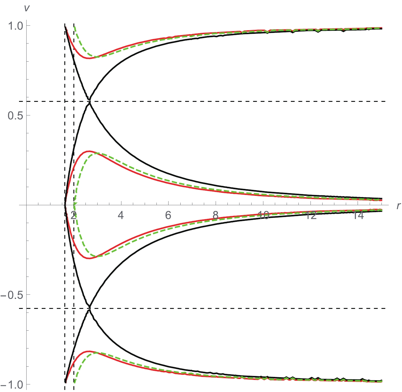
Figure 4. (color online) Contour lines of
${\cal{H}}^{\rm (AS)} = {\cal{H}}_{c}^{\rm (AS)}$ (black) and${\cal{H}}^{\rm (AS)} = {\cal{H}}_{c}^{\rm (AS)}\pm 0.06$ (red) for accretion of radiation:$ k = 1/3 $ . The green dashed curve is the contour line of${\cal{H}}^{\rm (GR)} = {\cal{H}}_{c}^{\rm (GR)}\pm 0.06$ . For all the orbits:$ M = 1 $ ,$ \xi = 0.5 $ . The vertical dashed lines locate the horizons$r_{\rm hIR}$ (left) and$r_{\rm hS}$ (right). The horizontal dashed lines locate the speed of sound$ a = \sqrt{k} $ . -
For sub-relativistic fluid, we have
$ r_c^{\rm (AS)}\simeq \frac{7}{2}M-\frac{26}{49}\frac{\xi}{M}, \qquad r_c^{\rm (GR)} = \frac{7}{2}M $

(34) and
$ {\cal{H}}^{\rm (AS)} = \frac{\Bigg(1-\dfrac{2M}{r}+\dfrac{2M\xi}{r^3}\Bigg)^{3/4}}{rv^{1/2}(1-v^{2})^{3/4}}, \quad {\cal{H}}^{\rm (GR)} = \frac{\Bigg(1-\dfrac{2M}{r}\Bigg)^{3/4}}{rv^{1/2}(1-v^{2})^{3/4}}. $

(35) The contour plots for
${\cal{H}}^{\rm (AS)}$ (continuous lines) and of${\cal{H}}^{\rm (GR)}$ (dashed line) in Fig. 5 show that, once again, the overall behavior of the contour lines is the same as in the two previous cases, with the same global quantum gravity effects on the accretion and outflow processes. Notwithstanding, we observe that for large values of$ r $ $ (r>r_c) $ , the quantum effects are milder for sub-relativistic matter than for ultra-relativistic and radiation fluids.
Figure 5. (color online) Contour lines of
${\cal{H}}^{\rm (AS)} = {\cal{H}}_{c}^{\rm (AS)}$ (black) and${\cal{H}}^{\rm (AS)} = {\cal{H}}_{c}^{\rm (AS)}\pm 0.06$ (red) for accretion of sub-relativistic fluid:$ k = 1/4 $ . The green dashed curve is the contour line of${\cal{H}}^{\rm (GR)} = {\cal{H}}_{c}^{\rm (GR)}\pm 0.06$ . For all the orbits:$ M = 1 $ ,$ \xi = 0.5 $ . The vertical dashed lines locate the horizons$r_{\rm hIR}$ (left) and$r_{\rm hS}$ (right). The horizontal dashed lines locate the speed of sound$ a = \sqrt{k} $ .At this point, it is important to show more explicitly how quantum effects modify accretion, that is, the dependence of the accretion flow on the parameter
$ \xi $ . This is displayed in Fig. 6 for the case of accretion of ultra-relativistic fluid ($ k = 1/2 $ ) and for subsonic flow. With the increase in the value of$ \xi $ (from right to left in the figure), the effects of shifting of the orbit and of increasing of the maximum flow velocity, already mentioned, become increasingly pronounced, whereas in the opposite limit,$ \xi \rightarrow 0 $ , the classical orbit is retrieved.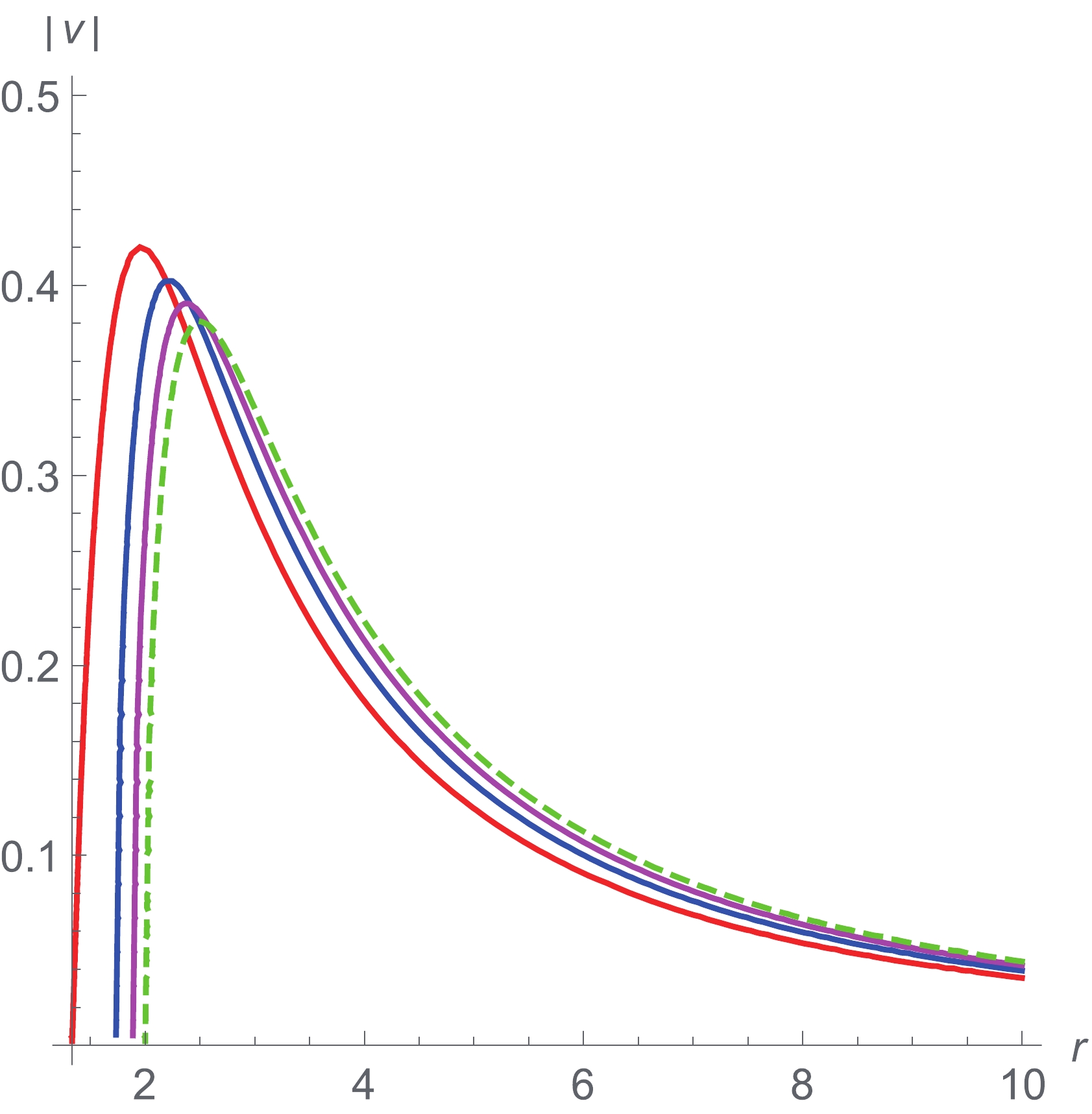
Figure 6. (color online) Orbits of
${\cal{H}}^{\rm (AS)} = {\cal{H}}_{c}^{\rm (AS)}\pm 0.06$ for subsonic accretion of ultra-relativistic fluid ($ k = 1/2 $ ) and for$ \xi = \xi_c = 16/27 $ (red),$ \xi = 0.4 $ (blue),$ \xi = 0.2 $ (magenta). The green dashed curve is the contour line of${\cal{H}}^{\rm (GR)} = {\cal{H}}_{c}^{\rm (GR)}\pm 0.06$ ($ \xi = 0 $ ). For all the orbits$ M = 1 $ . -
Let us start, following [30, 31], by writing the equations describing the accretion process in a more appropriate manner for the stability analysis.
First, the explicit form of the continuity equation reads
$ \begin{array}{l} \partial_{t}\left(\eta u^t\right)+ r^{-2} \partial_{r} \left(\eta u^r r^2\right) = 0. \end{array}$

(36) To solve for
$ \eta $ and$ u^r $ , we use the equation for energy-momentum conservation and the thermodynamic equation for mass-energy conservation${\rm d} (\epsilon/\eta)+P {\rm d} (1/\eta) = T {\rm d} s$ . Along with the condition of constant entropy${\rm d}s = 0$ , and with the square of the speed of sound given by Eq. (10), the condition of energy-momentum conservation reads$ \begin{aligned}[b] u^t \partial_{t} u^t &+ u^r \partial_{r} u^t + f\left(\partial_{r}f\right)u^r u^t \\ & + \frac{a^2}{\eta}\left[\left((u^t)^2- f\right)\partial_{t}\eta + u^r u^t \partial_{r}\eta\right] = 0. \end{aligned} $

(37) Once the expression for the speed of sound
$ a $ of the particular test fluid is known and after fixing the time derivatives to zero, the solution to the system of coupled equations (36) and (37) provides us with the stationary fields$ u^r(r) $ ,$ \eta(r) $ , and$ a(r) $ and allow, in principle, the quantitative study of the spherical accretion onto a static spherically symmetric black hole. Assuming that the flow is smooth at all points of space-time, the stationary solutions of Eqs. (36) and (37) are written as$ \begin{array}{l} 4\pi \bar{\mu} \eta u^r r^2 = \dot{m}, \end{array}$

(38) and
$ \frac{{\rm d}}{{\rm d}r}\left[\ln \left(f u^t \right)\right]+\frac{a^2}{\eta}\frac{{\rm d} \eta}{{\rm d}r} = 0, $

(39) respectively, where the constant of motion
$ \dot{m} $ is to be identified as the matter flow rate.The use of the perturbation scheme based on the continuity equation starts by considering linear perturbations to the stationary velocity and particle number density fields
$ u^r(r,t) = u^r(r) + u^{r \prime}(r,t) $ and$ \eta(r,t) = \eta(r) + \eta^\prime(r,t) $ , where primed quantities stand for small time-dependent perturbations. We now define the variable$ \psi = \eta u^r r^2 $ , whose stationary value$ \psi(r) $ coincides, except for the constant$ 4 \pi \bar{\mu} $ , with the steady mass accretion rate given by Eq. (38).The first order perturbation to
$ \psi $ around stationary values is$ \begin{array}{l} \psi^\prime(r,t) = [u^r(r) \eta^\prime(r,t) + \eta(r) u^{r \prime}(r,t)] r^2, \end{array}$

(40) and Eq. (36) acquires the form
$ u^t \partial_{t} \eta^{\prime} + \frac{\eta u^r}{f^2 u^t} \partial_{t} u^{r\prime} = - \frac{1}{r^2} \partial_{r} \psi^{\prime}. $

(41) In general, the first order perturbation to the square of the speed of sound is given by
$ a^{\prime 2} = a^2 + \frac{{\rm d}a^2}{{\rm d}\eta}\eta^{\prime}, $

(42) The time evolution of
$ \eta^{\prime} $ and$ u^{r\prime} $ follows from Eqs. (40) and (41) and is given, respectively, by$ \partial_{t} \eta^{\prime} = - \frac{1}{r^2} \left(\frac{u^r}{f} \partial_{t} \psi^{\prime} + f u^t \partial_{r} \psi^{\prime} \right), $

(43) $ \partial_{t} u^{r\prime} = \frac{f u^t}{\eta r^2} \left(u^t \partial_{t} \psi^{\prime} + u^r \partial_{r} \psi^{\prime} \right). $

(44) Eq. (37) is written in terms of perturbed quantities in the form
$ \begin{aligned}[b] u^t \left[u^r \frac{a^2}{\eta}\partial_{t} u^{r\prime} +\partial_{t} \eta^{\prime} \right] &+ \partial_{r}\left(u^r u^{r\prime} \right) + 2u^r u^{r\prime}\frac{a^2}{\eta} \partial_{r} \eta \\ & +(fu^t)^2 \partial_{r} \left(\frac{a^2}{\eta} \eta^{\prime} \right) = 0. \end{aligned} $

(45) Taking the time derivative of this last equation and substituting for the time derivatives of
$ \eta^{\prime} $ and$ u^{r\prime} $ from Eqs. (43) and (44), we obtain the differential equation obeyed by the perturbation to the mass accretion rate$ \psi^\prime $ $ \begin{aligned}[b] & \partial_{t} \left(\eta h^{tt} \partial_{t} \psi^{\prime} + \eta h^{tr}\partial_{r} \psi^{\prime} \right) + \partial_{r} \left(\eta h^{rt}\partial_{t} \psi^{\prime} + \eta h^{rr}\partial_{r} \psi^{\prime} \right) \\ =& (1 - 2a^2) \left(h^{rt}\partial_{t} \psi^{\prime} + h^{rr}\partial_{r} \psi^{\prime} \right)\frac{{\rm d}\eta}{{\rm d}r}, \end{aligned} $

(46) where the coefficients
$ h^{\alpha\beta} $ are given by$ \begin{aligned}[b] h^{tt} =& \frac{u^r (fu^t)}{f^2} \left[(fu^t)^2 + u^r - (u^r)^2 a^2 \right], \\ h^{tr} = & h^{rt} = \frac{(u^r)^2(fu^t)^2}{f}(1 - a^2), \\ h^{rr} =& u^r (fu^t) \left[(u^r)^2 - (fu^t)^2 a^2 \right]. \end{aligned} $

(47) -
Concerning the study of perturbations in the form of a standing wave, it is has been already pointed out in the literature that, because an event horizon instead of a physical surface occurs in a black hole, difficulties appear in fixing an appropriate inner boundary condition. Regularity of the flow at the black hole horizon singles out a unique solution, the Bondi one, which turns out to be transonic after crossing of the sonic point. However, the standing wave perturbation must vanish even in the supersonic regime, but there is no physical mechanism that allows to impose such a constraint. Because the standing wave analysis requires cancellation at the boundaries and the continuity of the solution, we must restrict ourselves to completely subsonic flows even though these may not entirely be representative of the precise manner of the infalling process. Consequently, in this section, we study the stability of a subsonic flow by assuming the trial standing wave perturbation
$ \begin{array}{l} \psi^{\prime}(r,t) = \zeta(r) \exp\left(-{\rm i}\omega t\right), \end{array}$

(48) which, when substituted into Eq. (46), provides
$ \begin{aligned}[b] \omega^2 h^{tt} \zeta^2 &+ {\rm i}\omega \left\{\frac{{\rm d}}{{\rm d}r} \left(h^{tr} \zeta^2 \right) - 2 h^{rt} \zeta^2 \frac{{\rm d}}{{\rm d}r}\left[\ln (f u^t) \right]\right\}\\& + \frac{h^{rr}}{(fu^t)^2} \frac{{\rm d}\zeta}{{\rm d}r} \frac{{\rm d}}{{\rm d}r}\left[\zeta (fu^t)^2\right] - \frac{{\rm d}}{{\rm d}r}\left(h^{rr}\zeta \frac{{\rm d} \zeta}{{\rm d}r}\right) = 0. \end{aligned}$

(49) Integrating Eq. (49) over the radial coordinate with the integrated terms vanishing at the boundaries, a dispersion relation for
$ \omega $ is obtained$ \begin{array}{l} A \omega^2 - 2 {\rm i} B \omega + C = 0 \end{array}$

(50) where
$ \begin{aligned}[b] A = & \int h^{tt} \zeta^2 {\rm d}r,\\ B = & \int h^{rt}\zeta^2 \frac{{\rm d}}{{\rm d}r} \left[ \ln \left(fu^t \right) \right]{\rm d}r, \\ C = & \int \frac{h^{rr}}{(fu^t)^2} \frac{{\rm d}\zeta}{{\rm d}r} \frac{{\rm d}}{{\rm d}r}\left[\zeta (fu^t)^2 \right]{\rm d}r. \end{aligned} $

(51) The roots of Eq. (50) are given by
$ \omega = {\rm i} \frac{B}{A} \pm {\rm i} \sqrt{\dfrac{B^2}{A^2}+\dfrac{C}{A}}. $

(52) Clearly, the sign of the discriminant of the relation dispersion determines the stability of the standing wave. Now, from Eq. (47), it follows that
$ h^{rt}>0 $ . Further, taking into account that for infalling matter$({\rm d}\eta/{\rm d}r) < 0$ , and referring to Eq. (39), we can conclude that$ B>0 $ . Again, because$ u^t = \sqrt{f+(u^r)^2}/f $ and for infalling fluid$ u^r<0 $ , we have$ h^{tt}<0 $ , which means$ A<0 $ . Finally, it is easily verified that for subsonic flow,$ h^{rr}>0 $ . Consequently,$ (B/A)<0 $ and$ (C/A)<0 $ , which implies whether an oscillatory and damped in time perturbation when$ \vert C/A \vert > (B/A) $ , or an overdamped perturbation if$ \vert C/A \vert < (B/A) $ . Thus, in any case, the stationary solution will be stable.Our goal, however, is to determine if quantum gravity effects enhance or diminish the dissipative effect associated to the coupling of the flow with the geometry of space-time. Nevertheless, since the integrands in the coefficients in Eq. (51) depend in a complicated manner on the classical and quantum functions
$ f_0(r) $ and$ f(r) $ , the solution for$ \omega $ is rather impractical for our purpose in the sense that it requires a considerable numerical effort after choosing a suitable mathematical distribution for modeling the amplitude of the standing wave. In the next section, we will see that this aim can be achieved more easily by analyzing a disturbance in the form of traveling wave. -
In this case, the perturbation will be modeled as a high-frequency traveling wave with a wavelength significantly smaller than the horizon radius of the black hole [19]. Then, the spatial part
$ \zeta(r) $ of the perturbation$ \psi^{\prime}(r,t) $ is written as a power series in$ \omega $ in the form [30, 31]$ \zeta_{\omega}(r) = {\rm exp} \left[\displaystyle\sum\limits_{l = -1}^{\infty} \omega^{-l}k_l(r)\right]. $

(53) After replacing into Eq. (49), the coefficients of
$ \omega^2 $ and$ \omega $ can be collected and equated, each to zero. In this manner, two first order differential equations are obtained for$ k_{-1} $ and$ k_0 $ , respectively. Settingthe coefficients of$ \omega^0 $ likewise to zero, a second order differential equation is obtained for$ k_1 $ , in terms of$ k_{-1} $ and$ k_0 $ . The solutions for$ k_{-1} $ and$ k_0 $ read$ \begin{array}{l} k_{-1} = {\rm i} \int \left(h^{rr}\right)^{-1} \left[h^{tr}\pm\sqrt{\left(h^{tr}\right)^2-h^{rr}h^{tt}}\right]{\rm d}r, \end{array}$

(54) and
$ \begin{array}{l} k_0 = \ln \left\{(fu^t)^2\left[\sqrt{\left(h^{tr}\right)^2-h^{rr}h^{tt}}\right]^{-1}\right\}^{1/2}, \end{array}$

(55) while the differential equation for
$ k_1 $ is$ \begin{aligned}[b] & 2 \left(h^{rr} \frac{{\rm d}k_{-1}}{{\rm d}r} - {\rm i} h^{tr}\right) \frac{{\rm d}k_1}{{\rm d}r} + \frac{\rm d}{{\rm d}r} \left(h^{rr}\frac{{\rm d}k_0}{{\rm d}r}\right) \\ +& h^{rr}\frac{{\rm d}k_0}{{\rm d}r} \frac{\rm d}{{\rm d}r} \left[k_0 - 2\ln(fu^t) \right] = 0 . \end{aligned}$

(56) The power series can be truncated after these first three terms, as indicated by their asymptotic behavior given by
$ k_{-1} \sim r $ ,$ k_0 \sim \ln r $ , and$ k_1 \sim r^{-1} $ , which likewise shows that the self-consistency requirement$ \omega^{-l}\vert k_l(r) \vert \gg \omega^{-(l+1)}\vert k_{l+1}(r)\vert $ for the convergence of the series is fulfilled. Thus, we can write$ \begin{array}{l} \zeta_{\omega}(r) \approx {\rm exp} \left[ \omega^1 k_{-1}(r)+k_0(r)+\omega^{-1}k_1(r) \right], \end{array}$

(57) It is then clear that
$ k_{-1} $ and$ k_1 $ only contribute to the phase of the traveling wave, and that the most important contribution to the amplitude of the perturbation$ \psi^{\prime}(r,t) $ comes from$ k_0 $ . A direct calculation yields$ \begin{aligned}[b] \vert\zeta_{\omega}(r)\vert =& \chi \vert{\rm exp}\left[k_0(r) \right]\vert = \chi \left\lvert \frac{(fu^t)^2} {\sqrt{\left(h^{tr}\right)^2-h^{rr}h^{tt}}}\right\rvert^{1/2} \\ =& \chi \left[\frac{(u_t)^2}{(u^r)^2 a^2} \right]^{1/4} = \chi \left(\frac{1}{v^2 a^2} \right)^{1/4}, \end{aligned} $

(58) where
$ \chi $ is an arbitrary small real constant, and we have used Eq. (13). It must be noted that, due to the fact that for a spherically symmetric accretion,$ v $ never equals to zero, and since$ a $ is also different from zero,$ \zeta_{\omega} $ never diverges, such that the background solution is stable.The dependence of
$ \vert\zeta_{\omega}(r)\vert $ on the metric coefficient$ f $ makes the effect of the space-time geometry on the perturbation evident and determines the coupling between the accretion flow and the curvature of space-time. The differences between these effects in AS and in GR for the accretion of isothermal fluids are already evident from Eq. (58), because a higher value of the three-velocity of the accretion$ v $ is always accompanied by a lower value of$ \vert\zeta_{\omega}(r)\vert $ and vice versa. The variation of$ \vert\zeta_{\omega}(r)\vert $ with the radial distance to the black hole can be calculated by writing the Hamiltonian for each type of isothermal fluid as a polynomial equation in the three-velocity$ v $ . After fixing an appropriate value for the Hamiltonian, this equation can be solved, and the result can be inserted into Eq. (58). These polynomial equations for each value of the state parameter$ k $ , except for$ k = 1 $ for which the expression for$ v^2 $ is immediate, read$ w^2 - w + \frac{f(r)}{{\cal{H}}^2(r)r^4} = 0 \qquad (k = 1/2), $

(59) where
$ w = v^2 $ ;$ v^3 - v + \frac{f(r)}{{\cal{H}}^{3/2}(r)r^2} = 0 \qquad (k = 1/3), $

(60) and
$ x^4 - x - \frac{f(r)}{{\cal{H}}^{4/3}(r)r^{4/3}} = 0 \qquad (k = 1/4), $

(61) where
$ x = v^{2/3} $ .From the solutions to previous equations for each value of
$ k $ , we selected only the one corresponding to infalling or outflowing matter with velocity approaching zero at the infinite spatial. By replacing the chosen solutions into Eq. (58), we can construct the plots shown in Fig. 7 for subsonic flow (similar plots can also be done for transonic and supersonic flows). In this figure, the upper left panel shows that for an ultra-stiff fluid, the amplitude of the perturbation is larger in AS as compared with the amplitude in GR for all values of$ r $ ($r > r_{\rm hS}$ ) that is, for the same radial distance a locally static observer measures a larger amplitude in AS than in GR, thus leading to a lower stability of the accretion process in AS. This indicates that, for ultra-stiff fluid, the coupling of the infalling matter with the space-time geometry is weaker in AS than in GR, a result which is undoubtedly associated to the anti-screening character of the gravitational interaction in AS. For the remaining cases of isothermal accretion, namely$ k = 1/2 $ ,$ k = 1/3 $ , and$ k = 1/4 $ , the upper right panel, lower left panel, and lower right panel in Fig. 7, respectively, show that the amplitude of the perturbation in AS is detracted from its value in GR if$ r_{hS}<r<r_{\mathrm{cross}} $ and it is instead enhanced if$ r>r_{\mathrm{cross}} $ , where the value of$ r_{\mathrm{cross}} $ for each type of isothermal fluid is simply obtained by solving the equation for$ r $ , which equals the quantum amplitude with the classical one. This means that the coupling of the fluid with the space-time curvature, which acts on the perturbation in the manner of a dissipative effect, is stronger in AS than in GR for$ r<r_{\mathrm{cross}} $ and is weaker for$ r>r_{\mathrm{cross}} $ . Notably, for sub-relativistic fluid, the main effect is the reduction of the amplitude of the traveling wave perturbation with the consequent increase in the coupling of the fluid with the curvature of space-time. This result has been already reported in [68].
Figure 7. (color online) Behavior of amplitude of traveling wave perturbation
$ \vert\zeta_{\omega}(r)\vert $ in AS (red) versus GR (green) for accretion of ultra-stiff fluid (upper left panel), ultra-relativistic fluid (upper right panel), radiation fluid (lower left panel), and sub-relativistic fluid (lower right panel). The vertical dashed line stands for the horizon radius$r_{\rm hS}$ of the classical Schwarzschild black hole. The values of the parameters are${\cal{H}}^{\rm AS} = {\cal{H}}_c^{\rm AS}+0.01$ ,${\cal{H}}^{\rm GR} = {\cal{H}}_c^{\rm GR}+0.01$ ,$ M = 1 $ ,$ \xi = 0.5 $ ,$ \chi = 0.1 $ -
In this work, we reviewed the problem previously analyzed in Ref. [61] regarding the steady accretion onto a R-G improved Schwarzschild black hole in AS theory with higher derivatives. In this sense, the accretion process is considered as a quantum correction to the known spherically symmetric accretion in general relativity. As in [61], we used an isothermal fluid as our test fluid, and we have specialized to the cases: ultra-stiff fluid (
$ k = 1 $ ), ultra-relativistic fluid ($ k = 1/2 $ ), radiation fluid ($ k = 1/3 $ ), and sub-relativistic fluid ($ k = 1/4 $ ). Because our interest has been to describe the most general aspects of the problem, we neglected viscous effects, heat transport, fluid self-gravity, and effects associated to the back-reaction of the fluid on the geometry. By using the Hamiltonian dynamical system procedure introduced in [63-65], we have recovered the results by the authors in [61] for the accretion of ultra-stiff, radiation, and sub-relativistic fluids. However, in contrast to what was established in that study, we found that accretion of ultra-relativistic fluids are a physical possibility in AS. In fact, for this type of fluid, as for the others considered here, we found not only a shifting of the orbits of the Hamiltonian in the$ (v,r) $ plane towards the central object and an enhancement of the flow velocity near the black hole as compared to what happens in GR, but also subsonic, supersonic, and transonic regimes. This is an important result, as there seems to be no physical reason for the no physical significance of the accretion of an ultra-relativistic fluid in AS. As expected, the quantum effects on the accretion are fully governed by the parameter$ \xi $ in the RG-improved metric coefficient$ f(r) $ in Eq. (2) with the classical behavior recovered in the limit$ \xi \rightarrow 0 $ .We also analyzed the issue of the stability of the accretion and compared the results with the known stability of the accretion flow in classical general relativity. Using a perturbative procedure based on the continuity equation, the mass accretion rate of the infalling matter, considered as an isothermal fluid, has been subjected to small linear perturbations in the form of a standing and a traveling wave. For the standing wave perturbation, we conclude that, as in the general relativistic realm, the disturbance is damped in time, such that the accretion is stable. As for the traveling wave perturbation a simple criterion, based on the behavior of the coefficient
$ k_0 $ in the series expansion of the spatial part of the perturbation, has allowed us to compare between the quantum and the classical frameworks, and to reach to the conclusion that, where quantum gravity effects will have to be accounted for, the amplitude of the traveling wave perturbation for ultra-stiff fluid becomes enhanced as compared with the classical one. This indicates that the coupling of this type of fluid with the space-time curvature is weaker in AS than in GR. For ultra-relativistic, radiation, and sub-relativistic fluids, the amplitude of the perturbation is reduced or enhanced depending on whether the local observer is located in the immediate neighborhood of the black hole horizon or not, respectively. The value of the radial coordinate$ r_{\mathrm{cross}} $ at which this transition takes place can be easily calculated by solving the equation for$ r $ , which equates the classical amplitude with the quantum one. This means that the coupling of the accreting fluid with the geometry of the space-time, which is responsible for the damping of the perturbation, is stronger in the quantum case than in the classical one for$ r<r_{\mathrm{cross}} $ and weaker for$ r>r_{\mathrm{cross}} $ . Because the disturbed quantity is the mass accretion rate, a physical quantity that is measurable in principle, it would be highly interesting to study the possible observable effects that could be used to test asymptotic safety in the future. -
We acknowledge financial support from COLCIENCIAS through the project with code 50754 associated to the CONVOCATORIA 757 PARA DOCTORADOS NACIONALES 2016. We also acknowledge financial support from Universidad Nacional de Colombia through the project with code 36031 within the program for the institutional strengthening of scientific research.
Black holes in asymptotic safety with higher derivatives: accretion and stability analysis
- Received Date: 2021-02-23
- Available Online: 2021-07-15
Abstract: We review steady spherically symmetric accretion onto a renormalization group improved Schwarzschild space-time, which is a solution to an asymptotically safe theory (AS) containing high-derivative terms. We use a Hamiltonian dynamical system approach for the analysis of the accretion of four types of isothermal test fluids: ultra-stiff fluid, ultra-relativistic fluid, radiation fluid, and sub-relativistic fluid. An important outcome of our study is that, contrary to the claim in a recent work, there are physical solutions for the accretion of an ultra-relativistic fluid in AS, which include subsonic, supersonic, and transonic regimes. Furthermore, we study quantum corrections to the known stability of the accretion in general relativity (GR). To this end, we use a perturbative procedure based on the continuity equation with the mass accretion rate being the perturbed quantity. Two classes of perturbations are studied: standing and traveling waves. We find that quantum gravity effects either enhance or diminish the stability of the accretion depending on the type of test fluid and the radial distance to the central object.


 DownLoad: