


 Abstract
 HTML
HTML Reference
 Related
 PDF
PDF


-
Neutron stars (NS) consist of a solid crust at low densities and a homogeneous core in the liquid phase. It is known that the uniform liquid becomes unstable with respect to small-amplitude density oscillations when the density decreases from the high-density homogeneous core to the inhomogeneous crust. Consequently, phase transitions occur that are associated with the liquid-gas phase transition in asymmetric nuclear matter in the presence of electrons. The properties of the crust and crust-core phase transition play an important role in understanding certain astrophysical observations [1-5].
It is well known that the relativistic mean field (RMF) theory can successfully describe many nuclear phenomena and can explain the saturation mechanism of nuclear matter and the strong spin-orbit interaction in finite nuclei in a consistent way [6-10]. In recent years, instead of the traditional RMF theory, which is based on the effective interaction between Dirac nucleons via the exchange of mesons, the RMF model with point-coupling (PC) interactions [11-13], which neglects mesonic degrees of freedom and considers only interactions with zero range, has become an alternative approach for the description of nuclear matter and finite nuclei. It allows a simpler treatment of exchange terms to study the effects beyond the mean-field for nuclear low-lying collective excited states and provides more opportunities to investigate the relationship with non-relativistic approaches.
Within the thermodynamic approach, Ref. [14] has used a widely used density-dependent parametrization of the PC model, DD-PC1 [12], to study the crust-core transition. In recent years, the crust-core transition has also been studied within the Vlasov formalism method [15-18]. Ref. [17] shows that the Vlasov approach generally gives a lower prediction of the transition density than does the thermodynamic approach. Moreover, given small oscillations around the equilibrium state in the Vlasov approach, the imaginary frequency of the dispersion relation characterizes the unstable collective modes. Ref. [19] points out that the thermodynamic approach corresponds to the limit with the wave vector of collective modes tending to zero. Thus, the Vlasov approach is better than the thermodynamic one for investigating the dynamical instabilities of finite-size collective modes, which have been focused on by many works within various models [15, 16, 19-22]. In this work, based on the parametrization DD-PC1, we use the Vlasov formalism method to investigate the effects of the density dependence of the symmetry energy on the crust-core transition and dynamical instabilities appearing at the transition, considering the influences of finite temperature and neutrino trapping as well.
This article is organized as follows. In Sec. II and the Appendix, we describe the equations necessary for the present work. In Sec. III, the calculated results and some discussion are provided. Finally, the summary is presented in Sec. IV.
-
In this work, the Lagrangian for DD-PC1 parametrization reads
$ \begin{aligned}[b] \text{£} =& \bar{\psi}[\gamma^{\mu}\left({\rm i}\partial_{\mu}-eA_{\mu}\frac{1-\tau_3}{2}\right)-M]\psi\\ &-\frac{1}{2}\alpha_S(\hat{\rho})(\bar{\psi}\psi)(\bar{\psi}\psi)-\frac{1}{2}\delta_S(\partial_{\nu}\bar{\psi}\psi)(\partial^{\nu}\bar{\psi}\psi)\\ &-\frac{1}{2}\alpha_V(\hat{\rho})(\bar{\psi}\gamma^{\mu}\psi)(\bar{\psi}\gamma_{\mu}\psi)\\&-\frac{1}{2}\alpha_{tV}(\hat{\rho})(\bar{\psi}\vec{\tau}\gamma^{\mu}\psi)\cdot(\bar{\psi}\vec{\tau}\gamma_{\mu}\psi)\,\,, \end{aligned} $

(1) where
$ \psi $ is the Dirac spinor of baryons and$ A_{\mu} $ denotes the electromagnetic field. The coupling parameter$ \delta $ is considered to be constant, while$ \alpha $ s in the various spin-isospin channels are analytical functions with respect to the baryonic density$ \rho $ alone.The effective one-body Hamiltonian can be given by
$ h_i = \left\{\begin{split}&{\sqrt{M^{*2}+(\vec{p}-\vec{V}^i)^2}}+V^{i0}\,\,, \;\;\;\;{\rm{for}}\;i = p,n\,\,,\\& \sqrt{m_e^{2}+(\vec{p}+e\vec{A})^2}-eA_0\,\,, \;\;\;\;{\rm{for}}\;i = e\,\,,\end{split}\right. $

(2) where the nucleon effective mass is defined as
$ M^* = M+\Sigma_S $ , and the scalar and vector self-energies,$ \Sigma_S $ and$ V^{i\mu} = \Sigma^{i\mu}_V+\Sigma^{\mu}_R $ , in which the rearrangement term$ \Sigma^{\mu}_R $ arises from the variation of the density-dependent vertex functionals with respect to the nucleon fields in the density operators, which can be given by$ \Sigma_S = \alpha_S\rho_S-\delta_S\triangle\rho_S\,\,, $

(3) $ \Sigma^{i\mu}_{V} = \alpha_Vj^{\mu}+\alpha_{tV}\tau_ij^{\mu}_3+e\frac{1+\tau_i}{2}A^{\mu}\,\,, $

(4) $ \Sigma_R^{\mu} = (\alpha'_S\rho_S^2+\alpha'_Vj_{\nu}j^{\nu}+\alpha'_{tV}j_{3\nu}j_3^{\nu})j^{\mu}/2\rho_V\,\,. $

(5) The Vlasov equation describes the time evolution of the one-body phase-space distribution functions for protons, neutrons, and electrons, denoted by
$ f_{i\pm}(\vec{r},\vec{p},t) $ , as$ \frac{\partial f_{i\pm}}{\partial t}+\{f_{i\pm},h_{i\pm}\} = 0\,\,,\,\,i = p,n,e, $

(6) where +(–) denotes particles (antiparticles) and {, } denotes the Poisson brackets. Small deviations of the distribution functions
$ \delta f $ around the equilibrium state can be obtained with generating functions S as$ \delta f_{i\pm} = \{S_{i\pm},f_{0i\pm}\} = \{S_{i\pm},p^2\}\frac{{\rm d}f_{0i\pm}}{{\rm d}p^2}\,\,, $

(7) where
$ f_{0i} $ are equilibrium distribution functions. Of particular interest are the longitudinal modes, with momentum$ \vec{k} $ and frequency$ \omega $ , described by the ansatz$ \left(\begin{array}{c}S_{i\pm}(\vec{r},\vec{p},t)\\ \delta\Sigma_S, \delta V^{i\mu}\\ \delta\rho_S, \delta j^{\mu},\delta j_3^{\mu}\\ \delta A^{\mu}\end{array}\right) = \left(\begin{array}{c}S^i_{\omega\pm}(p,\cos\theta)\\ \delta\Sigma^S_{\omega}, \delta V^{i\mu}_{\omega}\\ \delta\rho^S_{\omega}, \delta j^{\mu}_{\omega},\delta j^{\mu}_{3\omega}\\ \delta A^{\mu}_{\omega}\end{array}\right) {\rm e}^{{\rm i}(\omega t-\vec{k}\cdot\vec{r})}\,\,, $

(8) where
$ \theta $ is the angle between$ \vec{p} $ and$ \vec{k} $ . In terms of the generating functions, the linearized Vlasov equations for$ \delta f $ can be obtained. After transforming the unknowns$ S_{\omega} $ to density oscillations, we obtain the following matrix equation as$ M(\omega)\left(\begin{array}{c}\delta\rho^S_{\omega p}\\ \delta\rho_{\omega p}\\\delta\rho^S_{\omega n}\\ \delta\rho_{\omega n}\\\delta\rho_{\omega e}\end{array}\right) = 0\,\,, $

(9) where
$ \delta\rho^S_{\omega p} $ and$ \delta\rho^S_{\omega n} $ are the amplitudes of the oscillating scalar densities of protons and neutrons, respectively, and$ \delta\rho_{\omega p} $ ,$ \delta\rho_{\omega n} $ , and$ \delta\rho_{\omega e} $ are the amplitudes of the oscillating proton, neutron, and electron densities, respectively. The dispersion relation of collective modes is obtained from the determinant of$ M(\omega) $ . The derivation and the entries of$ M(\omega) $ are listed in Appendix A. -
In this work, the parameters of the isoscalar channels for DD-PC1 remain unchanged so that the properties of the saturated symmetric nuclear matter, namely, the saturation density, the binding energy, and the compression modulus, can be kept fixed. The symmetry energy for DD-PC1 is given by
$ E_{\rm sym} = \frac{k_F^2}{6\sqrt{k_F^2+M^{*2}}}+\frac{\alpha_{tV}}{2}\rho\,\,, $

(10) where
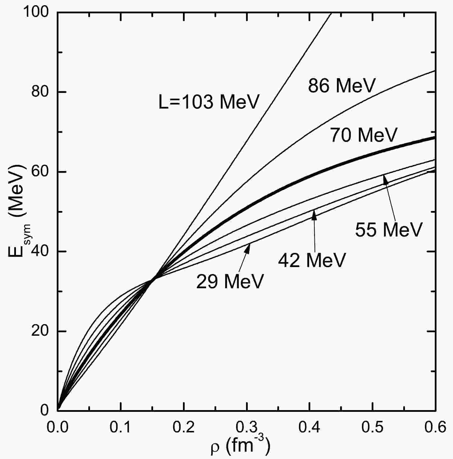
$ k_F $ is the Fermi momentum. In this work, we vary the density dependence of symmetry energy by adjusting the parameters of the isovector channels, i.e.,$ b_{tV} $ and$ d_{tV} $ in set C in Table 1 in Ref. [12], while keeping the symmetry energy at saturation unchanged by fixing$ \alpha_{tV} $ at saturation density in Eq. (10). We plot the symmetry energy$E_{\rm sym}$ as a function of the density for several values of the slope parameter of$E_{\rm sym}$ at saturation (parameter L) in Fig. 1. For larger L,$E_{\rm sym}$ is larger at supersaturation while smaller at subsaturation densities in comparison with another L. This density dependence of$E_{\rm sym}$ can likely explain the correlations between L and the crust-core transition.L/MeV T=0 MeV T=0 MeV 4 MeV 8 MeV 12 MeV $Y_{\nu}=0$ 

29 0.096 0.091 0.087 0.079 42 0.091 0.085 0.077 0.058 55 0.086 0.079 0.063 70 0.079 0.072 86 0.073 0.065 103 0.066 0.059 $Y_l=0.4$ 

29 0.095 0.087 0.086 0.081 0.07 42 0.094 0.086 0.085 0.08 0.068 55 0.094 0.085 0.084 0.079 0.066 70 0.093 0.084 0.083 0.078 0.065 86 0.093 0.084 0.083 0.077 0.063 103 0.093 0.083 0.082 0.076 0.062 Table 1. Crust-core transition densities [fm
$^{-3}$ ] for$\beta$ -equilibrium neutrino-free matter ($Y_{\nu}=0$ ) and neutrino-trapped matter ($Y_l=0.4$ ) for several slopes at saturation L and temperatures T including$T=0$ MeV. The results in italic type are for the thermodynamic method, and the other results are for the Vlasov approach. Those calculated with the original DD-PC1 parametrization are in bold type.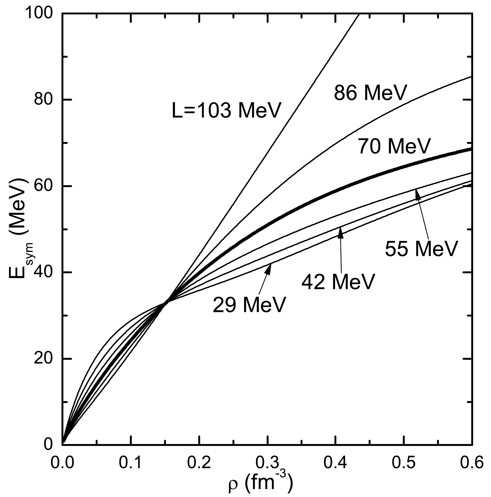
Figure 1. Symmetry energy
$E_{\rm sym}$ as a function of density$\rho$ for several values of L.$E_{\rm sym}$ at saturation is fixed at the original value (33 MeV) for DD-PC1. Thick curves are for original DD-PC1 parametrization with$L = 70$ MeV.In Tables 1-2, we show the transition densities
$ n_t $ and corresponding pressures$ P_t $ at the crust-core transition, respectively. The transition is defined as the crossing between the$ \beta $ -equilibrium line and the spinodal surface. The thermodynamic spinodal region requires the free energy curvature matrix to be negative, while the Vlasov spinodal surface corresponds to the solutions of the dispersion relation with frequency$ \omega = 0 $ and moment$ k = 75 $ MeV, where the chosen value of k in this work approximately defines the maximal spinodal region.L/MeV T=0 MeV T=0 MeV 4 MeV 8 MeV 12 MeV $Y_{\nu}=0$ 

29 0.265 0.225 0.275 0.42 42 0.417 0.349 0.346 0.378 55 0.489 0.393 0.284 70 0.485 0.365 86 0.404 0.282 103 0.283 0.182 $Y_l=0.4$ 

29 1.113 0.93 1.004 1.161 1.242 42 1.131 0.93 1.006 1.152 1.211 55 1.148 0.934 1.007 1.144 1.182 70 1.167 0.936 1.007 1.134 1.151 86 1.182 0.936 1.004 1.122 1.123 103 1.192 0.932 0.998 1.108 1.096 Table 2. Crust-core transition pressures [MeV fm
$^{-3}$ ] for several slopes at saturation L and temperatures T including$T=0$ MeV. The results in italic type are for the thermodynamic method, and the other results are for the Vlasov approach. Those calculated with the original DD-PC1 parametrization are in bold type.In Table 1, with the original DD-PC1 parametrization, the calculated
$ n_t $ for$ T = 0 $ MeV with the thermodynamic method are 0.079 and 0.093 fm$ ^{-3} $ for neutrino-free and neutrino-trapped$ \beta $ -equilibrium matter, respectively, while these values are approximately 10% larger than those determined using the Vlasov formalism method, which are 0.072 and 0.084 fm$ ^{-3} $ , respectively. The anticorrelation of$ n_t $ and L has been found in the literature using various methods [23-31]. Similarly, this table also shows that small L corresponds to a large value of$ n_t $ . It can be seen that$ n_t $ decreases with increasing temperature. Moreover, in the crust of neutrino-free matter, we see that there is no nonhomogeneous phase at temperatures greater than 4 MeV for$ L>70 $ MeV, and even for very low L, no nonhomogeneous phase exists at$ T = 12 $ MeV. This is primarily a result of the fact that the spinodal region can almost reach pure neutron matter at zero temperature, while it is more isospin symmetric for finite temperatures (see Fig. 1 of Ref. [20]). Meanwhile, the proton fraction of$ \beta $ -equilibrium neutrino-free matter is quite small at subsaturation, and the$ \beta $ -equilibrium line can only pass across the spinodal region marginally. Therefore, the crust-core transition is susceptible to changes in temperature. Figure 1 shows that a larger L corresponds to a smaller symmetry energy at subsaturation densities, thus favoring more neutron-rich matter for the homogeneous phase at subsaturation. As a result, the nonhomogeneous phase can only exist at a low temperature for a large L. By contrast, the proton fraction in the matter with trapped neutrinos is quite large, i.e.,$ \sim $ 0.3. Therefore, Table 1 shows that the transition densities do not differ much for various L and the nonhomogeneous phase still exists until$ T = 12 $ MeV, when neutrinos are trapped. This result means that the nonhomogeneous phase can exist at higher temperatures in the crust of a protoneutron star compared with that after neutrino outflow.In contrast with
$ n_t $ , the dependence of$ P_t $ on L is nontrivial, as shown in Table 2. At$ T = 0 $ MeV, for$ Y_{\nu} = 0 $ ,$ P_t $ increases with increasing L in the small L region ($ L\lesssim $ 55 MeV), and the opposite behavior occurs for$ L\gtrsim $ 55 MeV. This trend is similar to those observed in Refs. [17, 28, 29], while dissimialr to those in Refs. [27, 31]. For$ Y_l = 0.4 $ , the trend for the thermodynamic method is different and$ P_t $ increases monotonically with increasing L. Moreover, it is observed that$ P_t $ can move downward with increasing L when the temperature increases. These phenomena may arise from several competing effects, as discussed in Refs. [28, 29], and can be model dependent.It is known that the unstable modes correspond to the solutions of the dispersion relation with imaginary frequencies
$ \omega = i\Gamma $ , where$ \Gamma $ defines the exponential growth rate of the instabilities. With these solutions, we study the instability direction of the modes and the distillation effect, i.e., where the denser phase in nonhomogeneous nuclear matter prefers to be isospin symmetric. We plot the ratio of the proton over neutron density fluctuation$ \delta\rho_p/\delta\rho_n $ (upper panel) and the corresponding growth rate of collective modes (lower panel) at$ T = 4 $ MeV as a function of the wave vector k and the density$ \rho $ in Fig. 2 and Fig. 3, respectively. The proton fraction$ y_p = 0.3 $ chosen in both figures is close to the value in$ \beta $ -equilibrium matter with neutrino trapping. At large density ($ \rho = 0.5\rho_0 $ ) and small k ($ k = 10 $ MeV), both figures show small growth rates. We see in Fig. 2 that large L corresponds to a large distillation effect at$ \rho = 0.5\rho_0 $ . With decreasing density, the opposite behavior is found. This phenomenon can be seen in more clearly in Fig. 3, which shows that for$ \rho\gtrsim 0.05 $ fm$ ^{-3} $ , the large L increases the distillation effect, while at lower densities, the opposite occurs, i.e., lower L results in larger$ \delta\rho_p/\delta\rho_n $ . This result indicates that in the nonhomogeneous region near the inner boundary of the crust, where the densities are above a certain value, e.g., about 0.05 fm$ ^{-3} $ in this case, more proton-rich clusters are preferred for larger L, while in the lower-density region of the crust, the larger L leads to more neutron-rich clusters.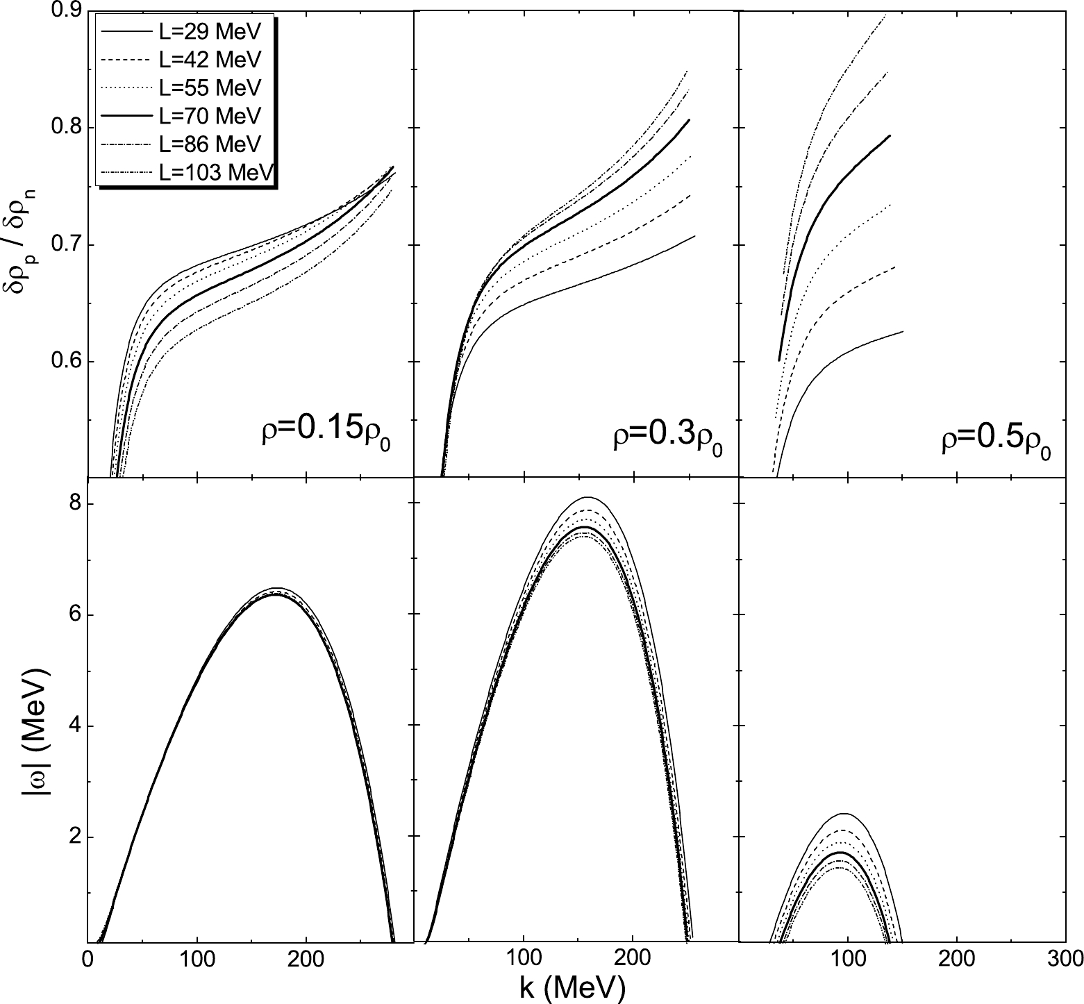
Figure 2. Ratio of the proton over neutron density fluctuation
$\delta\rho_p/\delta\rho_n$ (upper panel) and corresponding growth rate of collective modes (lower panel) as a function of the wave vector k, plotted for the proton fraction$y_p = 0.3$ ,$T = 4$ MeV, for$\rho = 0.15\rho_0$ ,$0.3\rho_0$ , and$0.5\rho_0$ . The saturation density$\rho_0 = 0.152$ fm$^{-3}$ . Thick curves are for original DD-PC1 parametrization.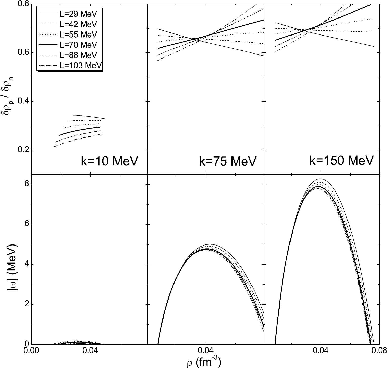
Figure 3. Same as Fig. 2, but as a function of the density
$\rho$ for wave vector k = 10, 75,150 MeV.The most unstable mode is taken as the mode with the largest growth rate
$|\omega|_{\max}$ , which drives the matter to the nonhomogeneous phase. Half of the wavelength$\lambda_{\max}/2$ associated with this mode is related to the most probable size of the clusters that are formed by the perturbation. We plot$|\omega|_{\max}$ (upper panels) and the corresponding$\lambda_{\max}/2$ (lower panels) as a function of density in$ \beta $ -equilibrium matter for free ($ Y_{\nu} = 0 $ ) and trapped neutrinos with a lepton fraction$ Y_l = 0.4 $ in Figs. 4 and 5, respectively, in which the results calculated with temperature$ T = 0 $ MeV, finite temperature$ T = 4 $ , 8, 12 MeV, and several values of L are chosen for comparison. We see from Fig. 4 that, except for very low densities, e.g.,$ \rho\lesssim 0.02 $ fm$ ^{-3} $ , a smaller value of L corresponds to alarger growth rate and smaller size of the clusters. With decreasing L, not only are the largest value of$|\omega|_{\max}$ and the smallest size of the clusters shifted to larger densities, but the density range for instabilities also increases. These phenomena can still be seen in Fig. 5. However, we see that the differences among various L are small because of the large proton fraction for matter with trapped neutrinos. Both figures show that the effects of the temperature are large and globally reduce the instability region and the growth rate while increasing the cluster size. The largest value of$|\omega|_{\max}$ and the smallest clusters are also observed to shift to larger densities with increasing temperature. Comparing these two figures, we see that the neutrino trapping leads to a large growth rate and small clusters, e.g., at T = 0 MeV, the smallest size of clusters is approximately 8-10 fm for neutrino-free matter, while this value is$ \thicksim $ 6 fm when including neutrinos.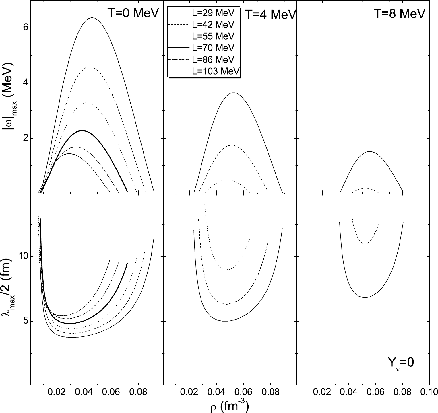
Figure 4. Growth rate of the most unstable modes (upper panel) and corresponding size of clusters (lower panel) as a function of density for
$\beta$ -equilibrium neutrino-free matter$Y_{\nu} = 0$ . Thick curves are for original DD-PC1 parametrization.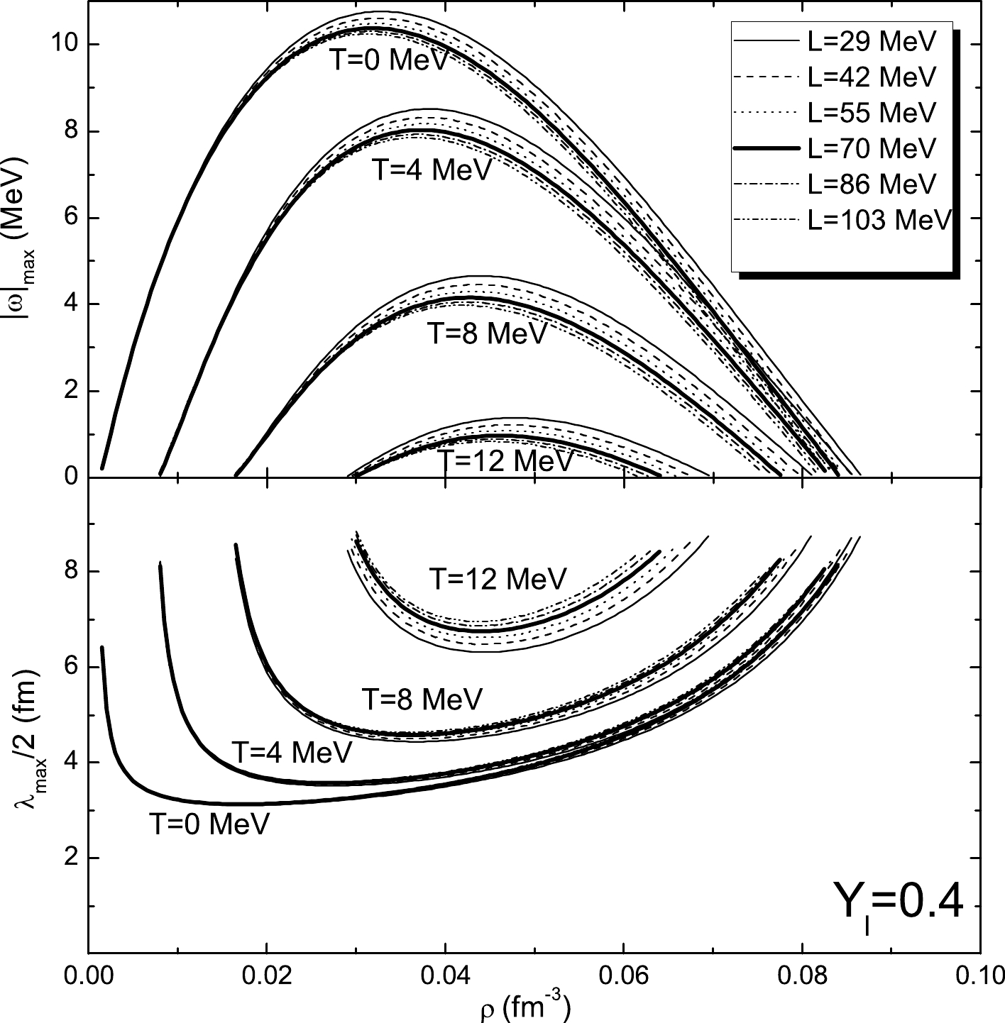
Figure 5. Same as Fig. 4, but for
$\beta$ -equilibrium neutrino-trapped matter$Y_l = 0.4$ . -
In summary, we have used the Vlasov formalism method to explore the effects of the density dependence of symmetry energy on the crust-core transition and dynamical instabilities in cold and warm neutron stars in the RMF theory with PC interactions. The role of neutrino trapping has also been considered. We see that
$ n_t $ decreases when L or the temperature increases, while neutrino trapping can diminish this effect due to the large proton fraction. However, their effects on$ P_t $ are nontrivial and model dependent. We observe that the clusters in the nonhomogeneous region near the inner boundary of the crust are preferentially more proton rich for larger L at$ \rho\gtrsim $ 0.05 fm$ ^{-3} $ , while in the lower-density region of the crust, the larger L leads to more neutron rich clusters. This phenomenon may affect the study of transport properties in the NS crust, such as electrical conductivity. The dynamical instability region, the size of clusters, and the growth rates have been estimated. The slope at saturation L, temperature, and trapping neutrinos have non-negligible effects. Finally, it needs to be mentioned that the nonhomogeneous phase, i.e., pasta phase, probably appears in the crust-core transition, where the spherical symmetry hypothesis within the Vlasov approach is thought to be broken. Thus, the conclusions for the clusters in the crust-core transition in this work need to be reexamined within other methods, e.g., as in Refs. [28, 29]. -
The oscillating baryon and scalar densities are given by
$\tag{A1} \begin{aligned}[b] \delta\rho_{\omega i} =& \frac{-1}{2\pi^2T}[M^*\delta\Sigma_{\omega}^{S}(I^{1i}_{\omega +}+I^{1i}_{\omega -})+\delta V^{0i}_{\omega}(I^{2i}_{\omega +}-I^{2i}_{\omega -}) \\ &-\frac{\omega}{k}\delta V^{i}_{\omega}(I^{2i}_{\omega +}-I^{2i}_{\omega -})]\,\,,\,\,i = p,n \end{aligned} $

$\tag{A2} \begin{aligned}[b] \delta\rho^S_{\omega i} =& \frac{-M^*}{2\pi^2T}[M^*\delta\Sigma_{\omega}^{S}(I^{0i}_{\omega +}-I^{0i}_{\omega -})+\delta V^{0i}_{\omega}(I^{1i}_{\omega +}+I^{1i}_{\omega -})\\ &-\frac{\omega}{k}\delta V^{i}_{\omega}(I^{1i}_{\omega +}+I^{1i}_{\omega -})]+c^i_S\delta\Sigma_{\omega}^{S}\,\,,\,\,i = p,n \end{aligned} $

where
$ \delta\Sigma_{\omega}^{S} $ ,$ \delta V^{0i}_{\omega} $ ,$ \delta V^{i}_{\omega} $ come from the variations of the scalar and vector self-energies with respect to the oscillating scalar and baryon densities in Eqs. (3)-(5) and$ c^i_S = \frac{2}{(2\pi)^3}\int {\rm d}^3p(f_{0i+}+f_{0i-})\frac{p^2}{\epsilon^3}\,\,, $

with
$ \epsilon = \sqrt{p^2+M^{*2}} $ , and the oscillating electron density is given by$ \tag{A3} \delta\rho_{\omega e} = \frac{e\delta A^0_{\omega}}{2\pi^2T}(I^{2e}_{\omega +}-I^{2e}_{\omega -})(1-\omega^2/k^2)\,\,,\,\, $

with
$ \tag{A4} (\omega^2-k^2)\delta A^0_{\omega} = -e(\delta\rho_{\omega p}-\delta\rho_{\omega e})\,\,, $

and
$ \tag{A5} I^{ni}_{\omega\mp} = \int^{\infty}_{m_i}\epsilon^nI_{\omega\mp}(\epsilon)f_{0i\mp}(f_{0i\mp}-1){\rm d}\epsilon\,\,, $

with
$ \tag{A6} I_{\omega\mp}(\epsilon) = \int^{p/\epsilon}_{-p/\epsilon}{\rm d}x\frac{x}{\omega/k\pm x}\,\,, $

in which
$ m_i $ denotes$ M^* $ for a nucleon and$ m_e $ for an electron. After straightforward but lengthy derivations, Eqs. (A1)-(A3) can be placed into a matrix equation, and the entries of$ M(\omega) $ in Eq. (9) are given by$\tag{A7} M(\omega ) = \left( {\begin{array}{*{20}{c}} {{a_{11}}}&{{a_{12}}}&{{a_{13}}}&{{a_{14}}}&{{a_{15}}}\\ {{a_{21}}}&{{a_{22}}}&{{a_{23}}}&{{a_{24}}}&{{a_{25}}}\\ {{a_{31}}}&{{a_{32}}}&{{a_{33}}}&{{a_{34}}}&0\\ {{a_{41}}}&{{a_{42}}}&{{a_{43}}}&{{a_{44}}}&0\\ 0&{{a_{52}}}&0&0&{{a_{55}}} \end{array}} \right){\mkern 1mu} {\mkern 1mu} .$

When the determinant of
$ M(\omega) $ is zero, the dispersion relation of collective modes is obtained, and the corresponding ratio of the proton over neutron density fluctuation$ \delta\rho_p/\delta\rho_n $ is given by$\tag{A8} \frac{\delta\rho_p}{\delta\rho_n} = -\frac{a_{11}A+a_{13}B+a_{14}}{a_{11}C+a_{13}D+a_{12}-a_{15}a_{52}/a_{55}}\,\,, $

with
$ \begin{aligned}[b] & A = \frac{a_{33}a_{44}-a_{34}a_{43}}{a_{31}a_{43}-a_{33}a_{41}}\,\,,\;\;\;\;B = \frac{a_{34}a_{41}-a_{31}a_{44}}{a_{31}a_{43}-a_{33}a_{41}}\,\,, \\& C = \frac{a_{33}a_{42}-a_{32}a_{43}}{a_{31}a_{43}-a_{33}a_{41}}\,\,,\;\;\;\;D = \frac{a_{32}a_{41}-a_{31}a_{42}}{a_{31}a_{43}-a_{33}a_{41}}\,\,. \end{aligned} $

For zero temperature, Eqs. (A1)-(A8) are still applicable in the present work when one replaces
$ I^{ni}_{\omega\mp} $ by$\tag{A9} I^{ni}_{\omega-} = 0\,\,,\frac{I^{ni}_{\omega+}}{T}\Rightarrow-\epsilon_{iF}^nI_{\omega+}(\epsilon_{iF})\,\,, $

in which
$ \epsilon_F $ is the Fermi energy at zero temperature.It is worth pointing out that in addition to the zero-range PC RMF models, the above equations Eqs. (A1)-(A9) can apply to finite-range meson-exchange RMF models. For the PC RMF models,
$ \delta\Sigma_{\omega}^{S} $ ,$ \delta V^{0i}_{\omega} $ , and$ \delta V^{i}_{\omega} $ in Eqs. (A1)-(A2) are functions with respect to the oscillating scalar and baryon densities, given by$ \begin{aligned}[b] \;\;\delta\Sigma_{\omega}^{S}=& c_{s0}\delta\rho^S_{\omega}+c_{s1}\delta\rho_{\omega} \,\,, \\ \delta V^{0i}_{\omega}=& c_{s1}\delta\rho^S_{\omega}+c^i_{v0}\delta\rho_{\omega}+c^i_{\rho0}\delta\rho_{\omega3}+e\frac{1+\tau_i}{2}\delta A^0_{\omega} \,\,, \\ \delta V^{i}_{\omega}=& \frac{\omega}{k}\left(c^i_{v1}\delta\rho_{\omega}+c^i_{\rho1}\delta\rho_{\omega3}+e\frac{1+\tau_i}{2}\delta A^0_{\omega}\right) \,\,, \end{aligned} $

where
$ \delta\rho_{\omega} = \delta\rho_{\omega p}+\delta\rho_{\omega n} $ ,$ \delta\rho_{\omega3} = \delta\rho_{\omega p}-\delta\rho_{\omega n} $ , and we have defined the following quantities as$ \begin{aligned}[b] c_{s0} = &\alpha_S+\delta_S(\omega^2-k^2)\,\,,\;\;\;\;\;\;\;\;\;\;\;\;c_{s1} = \alpha_S'\rho_S\,\,, \\ c_{v0}^i =& \alpha_V+2\alpha_V'\rho_V+\alpha_S''\frac{\rho_S^2}{2}+\alpha_V''\frac{\rho_V^2}{2}+\alpha_{tV}''\frac{\rho_3^2}{2}+\alpha_{tV}'\rho_3\tau^i\,\,, \\ c_{v1}^i =& \alpha_V+\frac{\alpha_S'\rho_S^2+\alpha_V'\rho_V^2+\alpha_{tV}'\rho_3^2}{2\rho_V}\,\,,\\ c_{\rho 0}^i =& \alpha_{tV}\tau^i+\alpha_{tV}'\rho_3\,\,,\;\;\;\;\;\;\;\;\;\;\;c_{\rho 1}^i = \alpha_{tV}\tau^i\,\,,\;\;\;\;\;\;\;\;\;(i = p,n) \end{aligned} $

with
$ \tau^p = 1 $ ,$ \tau^n = -1 $ ,$ \rho_3 = \rho_p-\rho_n $ . For meson-exchange RMF models, however, the variations of scalar and vector self-energies are functions with respect to the oscillating meson fields. The equations of motion of mesons have to be used to replace the oscillating meson fields by the oscillating densities in Eqs. A1-A2 to obtain the entries of$ M(\omega) $ .The coefficients
$ a_{ij} $ used in this work are given by$ a_{11} = 1+G_S^p(M^*c_{s0}(I^{0p}_{\omega +}-I^{0p}_{\omega -})+c_{s1}(I^{1p}_{\omega +}+I^{1p}_{\omega -}))\,\,, $

$ \begin{aligned}[b] a_{12} = &G_S^p\bigg\{M^*c_{s1}(I^{0p}_{\omega +}-I^{0p}_{\omega -})+\bigg[c_{v0}^p+c_{\rho 0}^p \\ & +\frac{\omega^2}{k^2}(c_{v1}+c_{\rho 1}^p)+\frac{e^2}{k^2}\bigg](I^{1p}_{\omega +}+I^{1p}_{\omega -})\bigg\}-g_V^p\,\,, \end{aligned} $

$ a_{13} = G_S^p(M^*c_{s0}(I^{0p}_{\omega +}-I^{0p}_{\omega -})+c_{s1}(I^{1p}_{\omega +}+I^{1p}_{\omega -}))-g_S^p\,\,, $

$ \begin{aligned}[b] a_{14} = &G_S^p\bigg\{M^*c_{s1}(I^{0p}_{\omega +}-I^{0p}_{\omega -})+\bigg[c_{v0}^p-c_{\rho 0}^p \\ &+\frac{\omega^2}{k^2}(c_{v1}-c_{\rho 1}^p)\bigg](I^{1p}_{\omega +}+I^{1p}_{\omega -})\bigg\}-g_V^p\,\,, \end{aligned} $

$ a_{15} = -G_S^p \frac{e^2}{k^2}(I^{1p}_{\omega +}+I^{1p}_{\omega -})\,\,, $

$ a_{21} = G_V(M^*c_{s0}(I^{1p}_{\omega +}+I^{1p}_{\omega -})+c_{s1}(I^{2p}_{\omega +}-I^{2p}_{\omega -}))\,\,, $

$ \begin{aligned}[b] a_{22} =& 1+G_V\bigg\{M^*c_{s1}(I^{1p}_{\omega +}+I^{1p}_{\omega -})+\bigg[c_{v0}^p+c_{\rho 0}^p \\ &+\frac{\omega^2}{k^2}(c_{v1}+c_{\rho 1}^p)+\frac{e^2}{k^2}\bigg](I^{2p}_{\omega +}-I^{2p}_{\omega -})\bigg\}\,\,, \end{aligned} $

$ a_{23} = G_V(M^*c_{s0}(I^{1p}_{\omega +}+I^{1p}_{\omega -})+c_{s1}(I^{2p}_{\omega +}-I^{2p}_{\omega -}))\,\,, $

$ \begin{aligned}[b] a_{24} =& G_V\bigg\{M^*c_{s1}(I^{1p}_{\omega +}+I^{1p}_{\omega -})+\bigg[c_{v0}^p-c_{\rho 0}^p \\ & +\frac{\omega^2}{k^2}(c_{v1}-c_{\rho 1}^p)\bigg](I^{2p}_{\omega +}-I^{2p}_{\omega -})\bigg\}\,\,, \end{aligned} $

$ a_{25} = -G_V \frac{e^2}{k^2}(I^{2p}_{\omega +}-I^{2p}_{\omega -})\,\,, $

$ a_{31} = G_S^n(M^*c_{s0}(I^{0n}_{\omega +}-I^{0n}_{\omega -})+c_{s1}(I^{1n}_{\omega +}+I^{1n}_{\omega -}))-g_S^n\,\,, $

$ \begin{aligned}[b] a_{32} =& G_S^n\bigg\{M^*c_{s1}(I^{0n}_{\omega +}-I^{0n}_{\omega -})+\bigg[c_{v0}^n+c_{\rho 0}^n \\ & +\frac{\omega^2}{k^2}(c_{v1}+c_{\rho 1}^n)\bigg](I^{1n}_{\omega +}+I^{1n}_{\omega -})\bigg\}-g_V^n\,\,, \end{aligned} $

$ a_{33} = 1+G_S^n(M^*c_{s0}(I^{0n}_{\omega +}-I^{0n}_{\omega -})+c_{s1}(I^{1n}_{\omega +}+I^{1n}_{\omega -}))\,\,, $

$ \begin{aligned}[b] a_{34} =& G_S^n\bigg\{M^*c_{s1}(I^{0n}_{\omega +}-I^{0n}_{\omega -})+\bigg[c_{v0}^n-c_{\rho 0}^n \\ & +\frac{\omega^2}{k^2}(c_{v1}-c_{\rho 1}^n)\bigg](I^{1n}_{\omega +}+I^{1n}_{\omega -})\bigg\}-g_V^n\,\,, \end{aligned} $

$ a_{41} = G_V(M^*c_{s0}(I^{1n}_{\omega +}+I^{1n}_{\omega -})+c_{s1}(I^{2n}_{\omega +}-I^{2n}_{\omega -}))\,\,, $

$ \begin{aligned}[b] a_{42} =& G_V\bigg\{M^*c_{s1}(I^{1n}_{\omega +}+I^{1n}_{\omega -})+\bigg[c_{v0}^n+c_{\rho 0}^n \\ &+\frac{\omega^2}{k^2}(c_{v1}+c_{\rho 1}^n)\bigg](I^{2n}_{\omega +}-I^{2n}_{\omega -})\bigg\}\,\,, \end{aligned} $

$ a_{43} = G_V(M^*c_{s0}(I^{1n}_{\omega +}+I^{1n}_{\omega -})+c_{s1}(I^{2n}_{\omega +}-I^{2n}_{\omega -}))\,\,, $

$ \begin{aligned}[b] a_{44} =& 1+G_V\bigg\{M^*c_{s1}(I^{1n}_{\omega +}+I^{1n}_{\omega -})+\bigg[c_{v0}^n-c_{\rho 0}^n \\ &+\frac{\omega^2}{k^2}(c_{v1}-c_{\rho 1}^n)\bigg](I^{2n}_{\omega +}-I^{2n}_{\omega -})\bigg\}\,\,, \end{aligned} $

$ a_{52} = -G_V \frac{e^2}{k^2}(I^{2e}_{\omega +}-I^{2e}_{\omega -})\,\,, $

$ a_{55} = 1+G_V \frac{e^2}{k^2}(I^{2e}_{\omega +}-I^{2e}_{\omega -})\,\,, $

with
$ G_V = \frac{1}{2\pi^2T}\,\,,\;\;\;\;\;\;G_S^i = \frac{M^*G_V}{1-c_{s0}c^i_S}\,\,,\;\;\;\;(i = p,n) $

and
$ g_V^i = \frac{c_{s1}c^i_S}{1-c_{s0}c^i_S}\,\,,\;\;\;\;g_S^i = \frac{c_{s0}c^i_S}{1-c_{s0}c^i_S}\,\,.\;\;\;\;(i = p,n) $

Crust-core transition and dynamical instabilities in neutron stars for model with point-coupling interactions
- Received Date: 2021-01-25
- Available Online: 2021-07-15
Abstract: We explore the effects of the density dependence of symmetry energy on the crust-core phase transition and dynamical instabilities in cold and warm neutron stars in the relativistic mean field (RMF) theory with point-coupling interactions using the Vlasov approach. The role of neutrino trapping is also considered. The crust-core transition density and pressure, distillation effect, and cluster size and growth rates are discussed. The present work shows that the slope of symmetry energy at saturation, temperature, and neutrino trapping have non-negligible effects.


 DownLoad: