Chiral symmetry restoration and deconfinement in the contact interaction model of quarks with parallel electric and magnetic fields

Dynamical chiral symmetry breaking and confinement are the two fundamental properties of non-perturbative quantum chromodynamics (QCD). At zero or low temperatures T, the fundamental degrees of freedom of quantum chromodynamics (QCD) are the low energy hadrons, whereas at high T, the interaction gets increasingly screened and thus becomes weak, causing hadrons to melt down to a new phase in which the predominant degrees of freedom are quarks and gluons. This phenomenon is referred to as the confinement–deconfinement phase transition. As the strength of the QCD interaction decreases with increasing T, only the current quark mass survives when the parameter T exceeds a critical value. This is termed as the chiral symmetry breaking–chiral symmetry restoration phase transition. Such a phase transition is expected to have occured in the early universe, a few microseconds after the Big Bang, and it is experimentally observed in heavy-ion collisions at the Large Hadron Collider (LHC) in CERN and Relativistic Heavy Ion Collider (RHIC) at Brook Heaven National Laboratory (BNL). In addition, when the hadronic matter is subjected to an external electromagnetic field background, it yields a significant impact on phase transition. It is well known that at $T = 0$, in the pure magnetic case, the strong magnetic field tends to strengthen the formation of quark anti-quark condensate, and the system remains in the chiral symmetry broken phase, even at a high magnetic field strength $eB$. This phenomenon is known as magnetic catalysis (MC) [1-10]. It was verified in earlier studies that at a finite T, the pseudo-critical temperature $T^{\chi, C}_c$ of the chiral symmetry restoration and deconfinement increases with an increase in $eB$; hence, magnetic catalysis is also observed at finite T [1, 2, 5, 11, 12]. Recently, the lattice QCD simulation [13-15] predicted that at finite T, a magnetic field suppresses the formation of quark-antiquark condensates and tends to restore the chiral symmetry at approximately the pseudo-critical temperature $T^{\chi, C}_c$. Consequently, $T^{\chi, C}_c$ decreases with an increase in $eB$, and such a phenomenon is known as the inverse magnetic catalysis (IMC). This phenomenon is validated and supported by effective models of low energy QCD [16-23], as well as in holographic QCD models [24].

In a pure electric case, and at $T = 0$, the situation is relatively different from that of a pure magnetic field background. The strong electric field suppresses the formation of a quark-antiquark condensate, and thus tends to restore the chiral symmetry, i.e., the electric field anti-screens the strong interaction. Such a phenomenon is known as the chiral electric inhibition effect [1, 2, 5, 11, 12, 25-28] or the chiral electric rotation effect [29]. The nature of chiral phase transitions is of the second order in the chiral limit but cross-over when the bare quark mass is considered. At finite temperature, it is well understood that the pseudo-critical temperature $T^{\chi, C}_c$ decreases with an increase in electric field strength $eE$, and this phenomenon is known as the inverse electric catalysis (IEC) [28, 30]. The study on the influence of electric fields on the chiral phase transitions, as well as the effect of the magnetic field, is equally important from theoretical and experimental perspectives. Experimentally, in heavy-ion collisions, the electric and magnetic fields are generated with the same order of magnitude ($\sim 10^{18}$ to$10^{20}$Gauss) [31-34] in the event-by-event collisions using Au $+$ Au at RHIC-BNL and in a non-central heavy-ion collision of Pb $+$ Pb in ALICE-LHC. Moreover, some interesting anomalous effects, such as the chiral magnetic [35, 36], chiral electric separation [37, 38], and particle polarization [39-41] effects, which may arise owing to the generation of vector and/or axial currents in the presence of strong electromagnetic fields, are also required for theoretical exploration. Recently, a special case of considering the electric field strength parallel to the magnetic field strength ($eE\parallel eB$) significantly focused on exploring the above-mentioned phenomenon in the effective models of QCD [28, 29, 42, 43]. A major reason behind this approach is that the parallel electric and magnetic fields play important and prominent roles in several heavy-ion collision experiments [44, 45].

Considering the aforementioned facts and findings, the objective of this study is to elucidate the traits of the dynamical chiral symmetry breaking-restoration transition in the presence of parallel electric and magnetic fields. The unified framework of this study is based on Schwinger-Dyson equations (SDE) in the rainbow-ladder truncation, Landau gauge, symmetry preserving the confining vector-vector contact interaction model (CI) [46], and Schwinger optimal time regularization scheme [47]. We adopt the quark-antiquark condensate $-\langle\bar{q}q\rangle$ as an order parameter for the chiral symmetry breaking-restoration, whereas for the confinement-deconfinement transition, we use the confinement length scale [22, 48]. It should be noted that the chiral symmetry restoration and deconfinement occur simultaneously in this model [22, 49].

This article is organized as follows. In Sec. II, we present the general formalism and contact interaction model at zero temperature, in the absence of background fields. In Sec. III, we discuss the gap equation at zero temperature, in the presence of parallel electric and magnetic fields presented in Sec. IV. Next, in Sec. V, we present the phase diagram at finite temperature, in the presence of parallel electric and magnetic fields. Finally, in Sec. VI, we present the summary and perspectives of this study.

We begin with the Schwinger-Dyson's equations (SDE) for a dressed-quark propagator $S_f$, which is given by

the subscript f represents the two light quark flavors, i.e., up (u) and down (d) quarks, g is the coupling constant, and $m_f$ is the current quark mass, which can be set to zero in the chiral limit. $\lambda^a$ represents the conventional Gell-Mann matrices, $\Gamma_\nu$ is the dressed quark-gluon vertex, and $\Delta_{\mu\nu}$ depicts the gluon propagator.

In literature, it is well known that the properties of low energy hadrons can be reproduced by assuming that the interaction among the quarks occurs not via a mass-less vector boson exchange but by the symmetry preserving four-fermions vector-vector CI with a finite gluon mass [46, 50-53]:

where $\alpha_{ ir} = 0.93\pi$ represents the infrared enhanced interaction strength parameter, and $m_G = 800$ MeV is the gluon mass scale [54]. In the CI model, for a small value of $\alpha_{ir}$ and a large value of the gluon mass scale $m_G$, there must be a critical value $\alpha_{\rm eff}$; above this critical value, the chiral symmetry is broken, and below this value, there is a lesser chance for the generation of the dynamical mass. The d-dimensional (arbitrary space-time dimensions) dependence of this effective coupling and its critical value on the chiral symmetry breaking, using an iterative method in the superstrong regime, has been comprehensively studied in Ref. [55].

The CI model Eq. (2), together with the choice of rainbow-ladder truncation $\Gamma_\nu(p,k) = \gamma_\nu$, forms the kernel of the quark SDE, Eq. (1), which brings the dressed-quark propagator into a very simple form [56]:

This is possible because the wave function renormalization trivially tends to unity in this case, and the quark mass function $M_f$ becomes momentum independent:

In this truncation, the quark-anitquark condensate is given by

with $N_c = 3$ representing the number of colors. The form of the proposed gap equation, Eq. (4), is significantly similar to the NJL model gap equation, except the coupling parameter $\alpha_{\rm eff} = \dfrac{9}{2} G$ [49].

Further simplification of Eq. (4) yields the following gap equation.

where $M_f$ represents the dynamical mass, and the symbol $\displaystyle\int^\Lambda$ stresses the need to regularize the integrals. Using ${\rm d}^4 k = (1/2) k^2 {\rm d}k^2 \sin ^2 \theta {\rm d}\theta \sin \phi {\rm d} \phi {\rm d}\psi$, and performing trivial regular integrations with the variable $s = k^2$, the above expression reduces to:

The integral in Eq. (7) is not convergent; therefore, we need to regularize it via the proper-time regularization scheme [47]. In this scheme, we take the exponent of the integrand's denominator and then introduce an additional infrared cutoff, in addition to the conventional ultraviolet cut-off, which is widely adopted in NJL model studies. Accordingly, the confinement is implemented using an infrared cut-off [57]. By adopting this scheme, the quadratic and logarithmic divergences are eliminated, and the axial-vector Ward-Takahashi identity [58, 59] is satisfied. From Eq. (7), the denominator of the integrand is given by

Here, $\tau_{uv}^{-1} = \Lambda_{uv}$ is an ultra-violet regulator that plays the dynamical role and sets the scale for all dimensional quantities. $\tau_{ir}^{-1} = \Lambda_{ir}$ represents the infrared regulator whose non zero value implements confinement by ensuring the absence of quarks production thresholds [60]. Hence, $\tau_{ir}$ corresponds to the confinement scale [22]. From Eq. (8), it is clear that the location of the original pole is at $s = -M^2$, which is canceled by the numerator. Accordingly, we discarded the singularities, and the propagator is free from real and complex poles, which is consistent with the definition of confinement: "an excitation described by a pole-less propagator would never reach its mass-shell" [57].

After performing integration over "s", the gap equation is given by

where

and $\Gamma(a,x) = \displaystyle\int_x^{\infty} t^{\alpha-1} {\rm e}^{-t} {\rm d}t$, which is the incomplete Gamma function. By using the parameters of Ref. [50], i.e., $\tau_{{ir}} = (0.24\; \mathrm{GeV})^{-1}$ and $\tau_{uv} = (0.905\; \mathrm{GeV})^{-1}$, with the bare quark $m_u = m_d = 0.007$ GeV, we obtain the dynamical mass $M_u = M_d = 0.367$ GeV and the condensate $\langle\bar{q}q\rangle_u = \langle\bar{q}q\rangle_d = -(0.0143)$ GeV$^3$.

In this section, we study the gap equation in the presence of a uniform and homogeneous electromagnetic field with $eE\parallel eB$ and at zero temperature. In the QCD Lagrangian, the interaction with the parallel electromagnetic field $A^{\rm ext}_\mu$ embedded in the covariant derivative is expressed as

where $Q_{f} = (q_u = +2/3 ,q_d = -1/3)e$ refers to the electric charges of u and d-quarks, respectively. We adopt the symmetric gauge vector potential $A^{\rm ext}_\mu = ({\rm i}\, E z, 0,-B x, 0)$ in Euclidean space, where both the electric and magnetic fields are selected along the z-axis. The gap equation in the presence of the parallel electromagnetic field remains in the form of Eq. (4), where $S_f(k)$ is dressed with parallel background fields, i.e., ${S_f}(k) \rightarrow\tilde{S_f}(k)$. $\tilde{S_f}(k)$, in the Schwinger proper time representation [1, 2, 5, 47], in the presence of the parallel magnetic field in Euclidean space [26, 29], is given by

where the magnetic field couples with the coordinate indices $1$ and $2$, while the electric field couples with $3$ and $4$. Now, taking the trace of Eq. (12) and introducing both infrared and ultraviolet cut-offs, the gap equation in the presence of parallel electric and magnetic fields is given by

The infrared cu-off $\tau_{ir}$ is introduced in the model to mimic confinement by ensuring the absence of quarks production thresholds. In the presence of both $eE$ and $eB$, it is required to vary slightly with both $eE$ and $eB$. Therefore, the entanglement between dynamical chiral symmetry breaking and confinement is expressed using an explicit $eE$ and $eB$-dependent regulator in the infrared [22]:

where $M_f$ is the dynamical mass in the absence of background fields, and $\tilde{M}_f$ represents the $eE$ and $eB$ dependent dynamical mass. For chiral quarks (i.e., $m_f = 0$), the confining scale $\tilde{\tau}_{ir}$ diverges at the chiral symmetry restoration parameter near its critical value, which ensures the simultaneity of deconfinement and chiral symmetry restoration [22]. After the integration over k, the gap equation, Eq. (13), can be written as

When both fields $eE$ and $eB \rightarrow 0$, Eq. (15) reduces to Eq. (9). The gap equation for the pure electric field can be obtained by setting $eB\to 0$, while for pure magnetic field, $eE\to 0$. The quark-antiquark condensate in the presence of background fields is in this form.

In this study, we adopt two flavors $f = 2$, i.e., u- and d-quarks. We use the same current quark mass for the up and down quarks, i.e., $m_u = m_d = 0.007$ GeV, such that the iso-spin symmetry is preserved. As is well-known, the response to the electromagnetic field is different for u and d-quarks because they have different electric charges [1, 5].

The numerical solution of the gap equation Eq. (15) as a function of $eB$ for fixed values of $eE$, is plotted inFig. 1. In the pure magnetic case ($eE\rightarrow0$), the dynamical mass $\tilde{M_f}$ monotonically increases with an increase in $eB$ , which ensures the magnetic catalysis phenomenon. The increase in $\tilde{M_f}$ as a function of $eB$ reduces in magnitude upon varying $eE$ from its smaller to larger given values. We noticed that at $eE\geqslant 0.33$ GeV$^2$, the dynamical mass $\tilde{M_f}$ exhibits the de Haas-van Alphen oscillatory type behavior [61]. In other words, it remains constant for small $eB$ values, then monotonically decreases with an increase in $eB$, and abruptly declines to lower values in the region $eB\approx[0.3-0.54]$ GeV$^2$, where the chiral symmetry is partially restored via first-order phase transition; above it, the value increases again. This phenomenon can be attributed to the strong competition that occurs between parallel $eB$ and $eE$, i.e., on the one hand, $eB$ enhances the mass function, while on the other hand, $eE$ suppresses it. We also sketch a zoom-in plot of the mass function, which shows the de Haas-van Alphen oscillatory behavior in the region $eB\approx[0.3-0.54]$ GeV$^2$ with $eE = 0.33$ GeV$^2$ , as illustrated in Fig. 2. Such a behavior type is also explored and discussed in the other effective model of QCD, for example, refer to Refs. [29, 62].

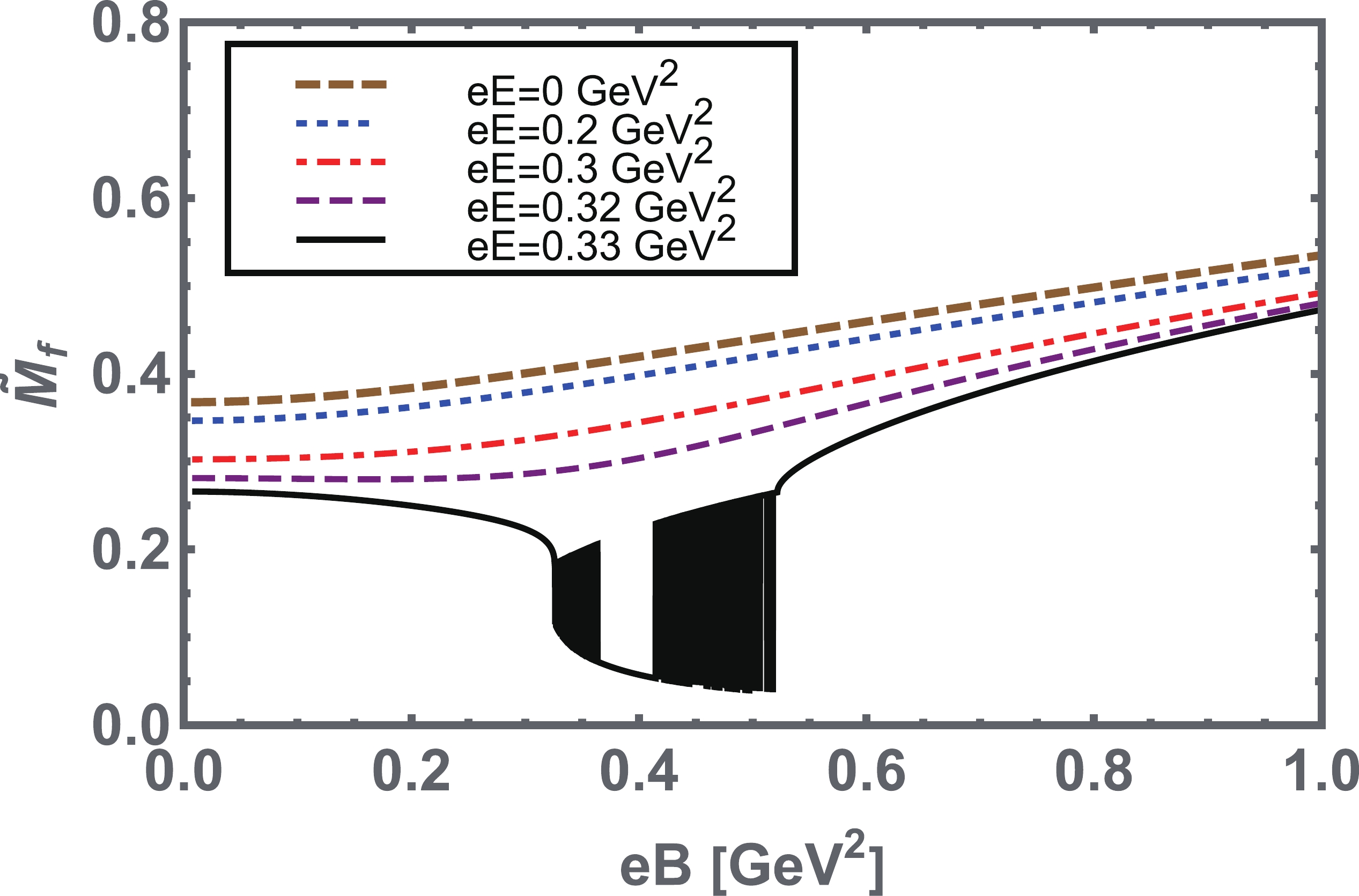
Figure 1.  (color online) Behavior of the dynamically generated quark mass, Eq. (15), as a function of the magnetic field strength $eB$ at several given values of $eE.$

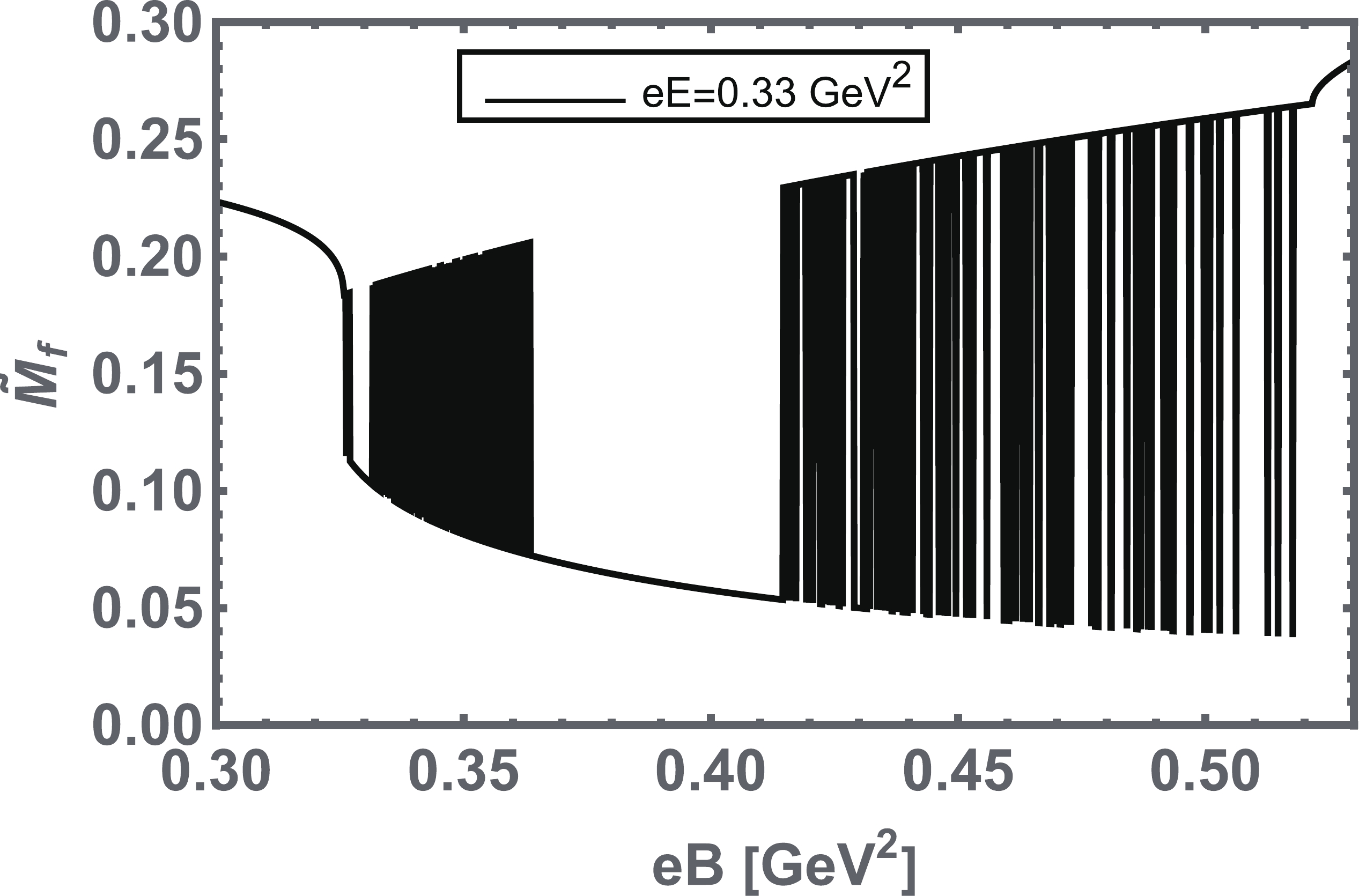
Figure 2.  Zoom-in plot of the mass function that shows the de Haas-van Alphen oscillatory behavior in the magnetic field region $eB = [0.3 - 0.5]$ GeV$^2$ with the electric field $eE = 0.33$ GeV$^2$

The behavior of the quark-antiquark condensate, Eq. (16), as a function of $eB$ at various given values of $eE$, is illustrated in the Fig. 3. For a pure magnetic case ($eE\rightarrow0$), the magnetic field strength $eB$ facilitates the formation of the quark-antiquark condensate. For given non zero values of $eE$, particularly, at $eE\approx 0.33$ GeV$^2$ the evolution in the condensate is suppressed in the region $eB = [0.3-$$0.54]$ GeV$^2$. The nature of the transition in this region suddenly changes to first-order; however, above this region, it is enhanced with $eB$. The pseudo-critical values of the fields at which the chiral symmetry partially is restored and first-order phase transition occurres are $eB_c\approx0.3$ GeV$^2$ and $eE_c = 0.33$ GeV$^2$. Although such values of electric or magnetic field strength are sufficiently large in terms of what is typically generated during heavy-ion collisions, they may be relevant to astronomical objects, such as neutron stars, magnetars, etc. The confinement parameter $\tilde{\tau}^{-1}_{ir}$ as a function of $eB$ for different fixed values of $eE$ is presented in Fig. 4. We observed the same pseudo-critical fields $eB_c\approx0.3$ GeV$^2$ and $eE_c =$$0.33$ GeV$^2$ for the confinement transition, similar to the case of chiral symmetry breaking.

Figure 3.  (color online) Quark-antiquark condensate, Eq. (16), as a function of $eB$ for several values of $eE.$

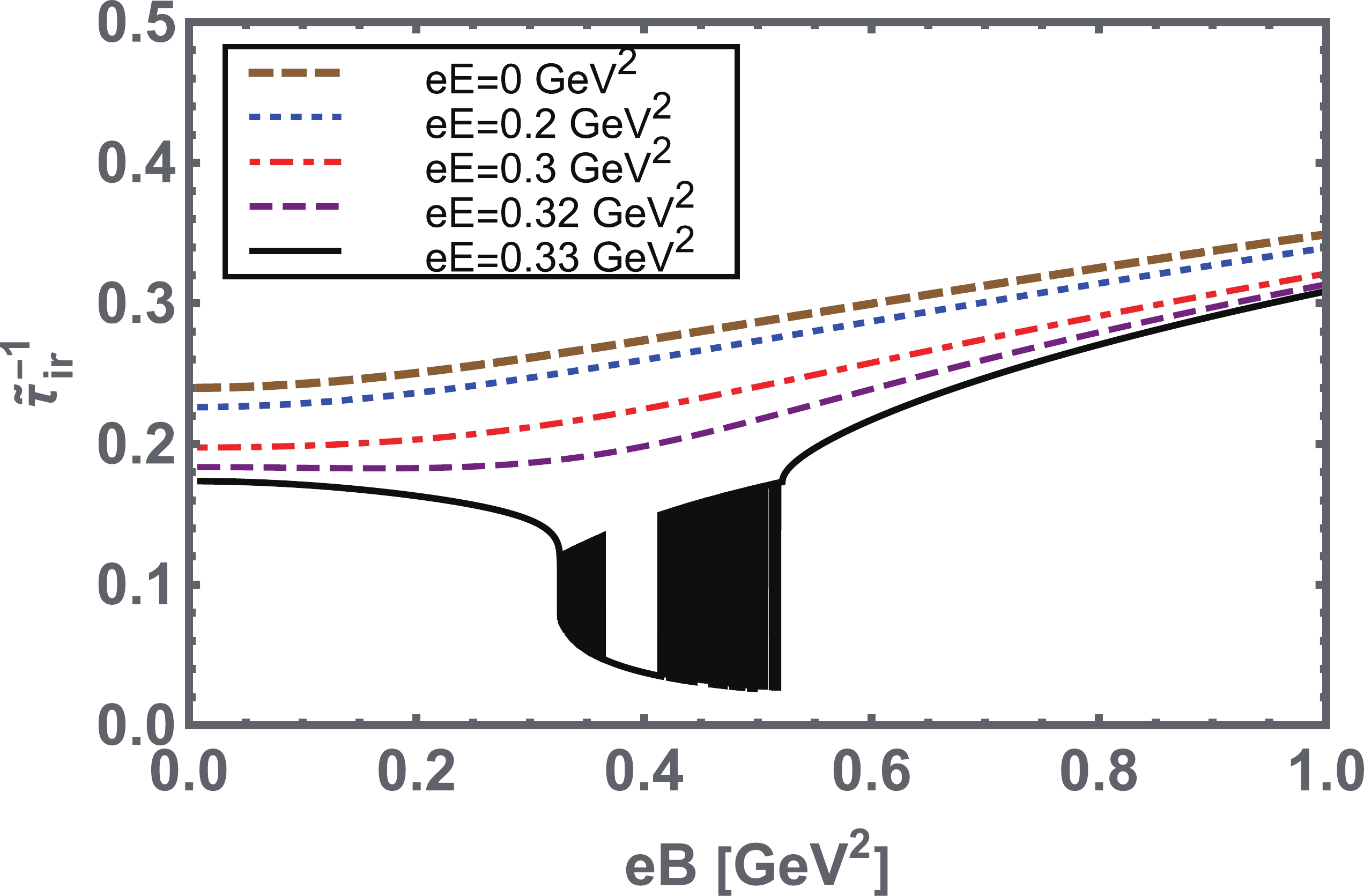
Figure 4.  (color online) Confinement scale $\tilde{\tau}^{-1}_{ir}$ as a function of $eB$ for several values of $eE.$

In the following, we discuss the variation of $\tilde{M_f}$ and $\tilde{\tau}^{-1}_{ir}$ as a function of $eE$, in the pure electric field, as well as for several non-zero values of $eB$. In Figs. 5, 6, and 7, we illustrate the behaviors of all three parameters as a function of $eE$, for various values of $eB\geqslant 0$.

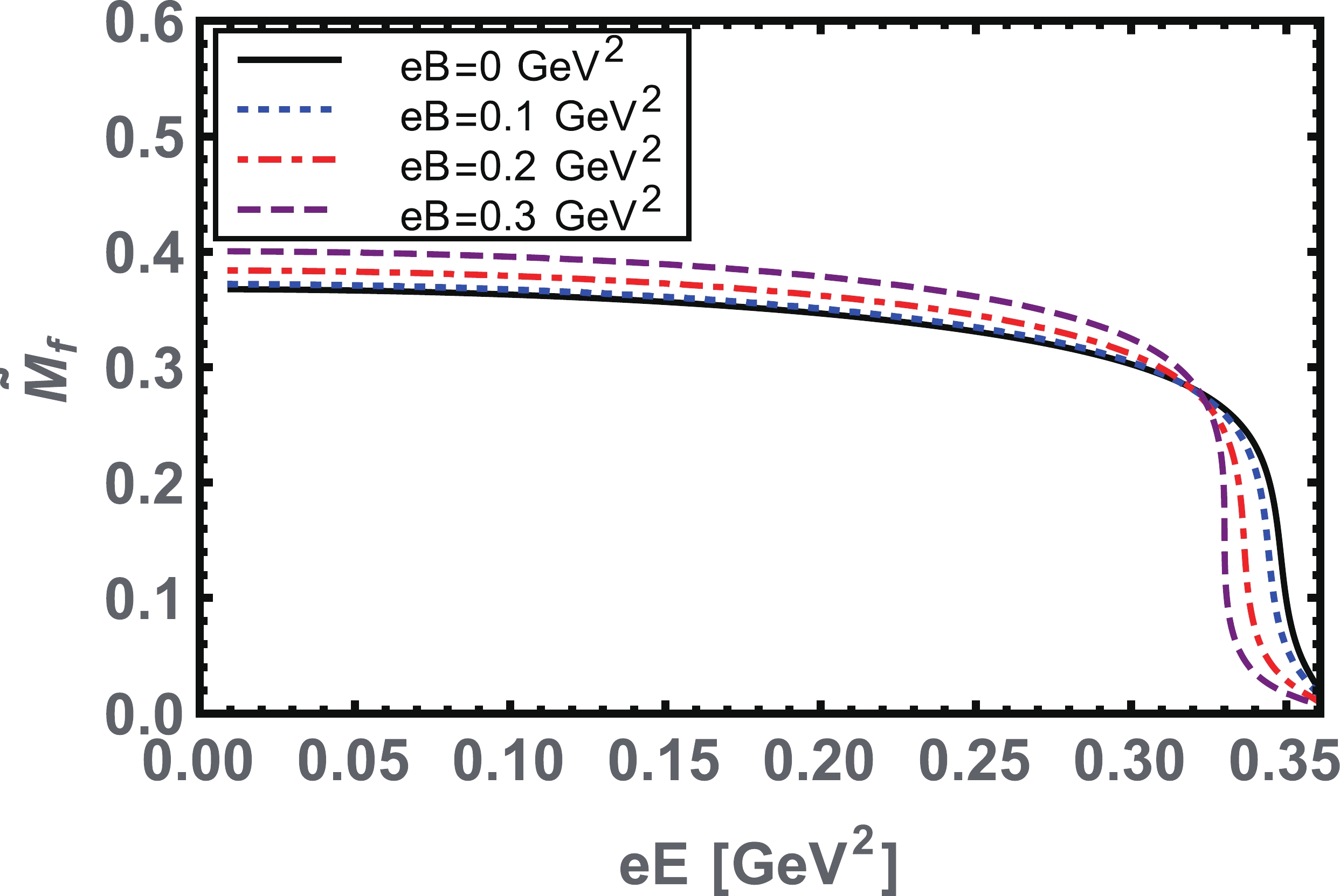
Figure 5.  (color online) Dynamical mass as a function of $eE$ for several values of $eB.$

Figure 6.  (color online) Quark-antiquark condensate, Eq. (16), as a function of $eE$ for several values of $eB.$

Figure 7.  (color online) Confinement scale $\tilde{\tau}^{-1}_{ir}$ as a function of $eE$ for a given several values of $eB.$

In the pure electric field case ($eB\rightarrow0$), the three-parameters monotonically decrease with an increase in $eE$, and at a pseudo-critical field strength $eE^{\chi, C}_c$ , the chiral symmetry is partially restored and deconfinement transitions occurred; hence, the nature of the transitions here becomes smooth cross-over. Accordingly, we observed the chiral rotation or chiral electric inhibition effect in the contact interaction model, as already predicted by other effective models of QCD [1, 2, 25-29]. For non-zero $eB$ values, we determined an interesting behavior for all the three parameters, as a function of $eE$. All three parameters are enhanced for given smaller to larger values of $eB$, except the chiral symmetry restoration and deconfinement regions, where all the parameters are suppressed by higher $eB$ values. The pseudo-critical field strength $E^{\chi, C}_{c}$ decreases with an increase in $eB$, and at a pseudo-critical $eB_c\approx 0.3$ GeV$^2$, the transition changes from cross-over to first order. The nontrivial behaviors of all three parameters represent the competition between the magnetic catalysis and electric inhibition effects, both induced by $eB$ in the presence of parallel $eE$ [29]. As elucidated and validated in Ref. [25], the cause of the chiral inhibition effect is the second Lorentz invariant of the electromagnetic field, ${E}\cdot {B}$. The magnitude of $eE^{\chi,C}_{c}$ at which the chiral symmetry restoration and deconfinement occurred are triggered from the inflection point of the electric gradients of $\textrm{and}\; \partial _{eE} \tilde{\tau}^{-1}_{ir}$, as presented in Figs. 8 and 9, respectively. In the pure electric case, the chiral symmetry restoration and deconfinement transition occur at $eE^{\chi,C}_{c}\approx0.34$ GeV$^2$. For several given values of $eB\neq0$, $eE^{\chi,C}_{c}$ decreases with an increase in $eB$. We determined a smooth cross-over phase transition up to the pseudo-critical magnetic field strength $eB_c\approx0.3$ GeV$^2$, where the transitions take the first-order nature. Here, $eE^{\chi,C}_{c}$ remains constant in the region $eB\approx[0.3-0.54]$ GeV$^2$ and then increases with larger values of $eB$ , as shown in Fig. 10. A similar behavior has already been demonstrated in [29]. The boundary point where the cross-over phase transition ends and the first order phase transition starts is known as a critical end point, and its co-ordinates are at $(eB_{p}\approx0.3,eE_{p}\approx0.33)$ GeV$^2$.

Figure 8.  (color online) Electric gradient of the quark-antiquark condensate as a function of $eE$ for fixed values of $eB$. At a particular fixed value of $eB^ = 0.3$ GeV$^2$, the electric gradient diverges at $eE^{\chi}_{c,}\approx0.33$ GeV$^2$ and above this value, the first order phase transition occurs.

Figure 9.  (color online) Electric gradient of the confinement scale $\partial _{eE} \tilde{\tau}^{-1}_{ir}$, as a function of $eE$ for different fixed values of $eB$. At a particular fixed value of $eB = 0.3$ GeV$^2$, the electric gradient of the confinement scale diverges at $eE^{C}_{c}\approx0.33$ GeV$^2.$

Figure 10.  (color online) Phase diagram of chiral symmetry and confinement for $eE^{C,\chi}_{c}$ vs $eB$. $eE = eE^{C,\chi}_{c}$ is obtained from the inflection points of the electric gradient of the condensate and the confining length scale $\partial _{eE} \tilde{\tau}^{-1}_{ir}.$

In this section, we elucidate the behaviors of the dynamical mass, condensate, and confinement length scale at a finite temperature and in the presence of parallel electric and magnetic fields. We also explore the IEC, MC, and IMC phenomena, as well as the competition among them. Finally, we sketch the QCD phase diagram.

The finite temperature version of the gap equation, Eq. (13), in the presence of parallel electric and magnetic fields can be obtained by adopting the standard convention for momentum integration:

and the four momenta $k\rightarrow(\omega_{n},\vec{k})$, with $\omega_n = (2n+1)\pi T$, represent the fermionic Matsubara frequencies. The Lorentz structure does not preserve anymore at finite temperature. By making the following replacements in Eq. (13),

and $k_{4}\rightarrow \omega_{n}$, we have

with $\hat{M}_f = {M}_f (eE, eB,T )$. Performing sum over Matsubara frequencies and integrating over $k's$, the gap equation can be written as

where ${\Theta_{3}}(\frac{\pi}{2},{{\rm e}^{-x}})$ is the third Jacobi's theta function. The confinement scale $\hat{\tau}_{ir}$ here slightly varies with T, $eE$ , and $eB$, and it takes the form

Here, $M_f = M_f(0,0,0)$ is the dynamical mass at $eB = eE = T = 0$, whereas $\hat{M}_f = {M}_f (eE, eB,T )$ is the variation of the dynamical mass at finite $eB$, $eE$, and T. The quark-antiquark condensate is given by the following.

First, we consider the case of a pure electric field at a finite temperature. The numerical solution of Eq. (19) as a function of T, for different given values of $eE$, is presented in Fig. 11. The dynamical mass $\hat{M}_f$ monotonically decreases with the increase of T until the dynamical chiral symmetry is partially restored. The response of $eE$ is to suppress the dynamical mass. The quark-antiquark condensate, Eq. (14), and confinement length scale, Eq. (15), as a function of T for various given values of $eE$ are depicted in Figs. 12 and 13, respectively. We infer that both parameters decrease with temperature T, and at a pseudo-critical temperature $T^{\chi, C}_c$, the chiral symmetry is partially restored, and deconfinement occurs. We note that the electric field $eE$ suppresses both parameters in the low-temperature regions and also reduces the pseudo-critical temperature $T^{\chi, C}_c$. In Figs. 14 and 15, we plotted the thermal gradients of the condensate and the confinement length scale, respectively. The peaks in the thermal gradients of both parameters shift toward the low-temperature regions upon increasing the value of $eE$. Consequently, the critical temperature $T^{\chi, C}_c$ decreases with an increase in electric field strength $eE$; hence, inverse electric catalysis is observed at a finite temperature in the proposed contact interaction model. Therefore, the observations of this study are consistent with other effective models of QCD [28-30]. The magnitude of the critical temperature $T^{\chi,C}_c\approx0.22$ GeV$^2$ is obtained from the inflection points of the thermal gradients of and $\partial _{T} \hat{\tau}^{-1}_{ir}$.

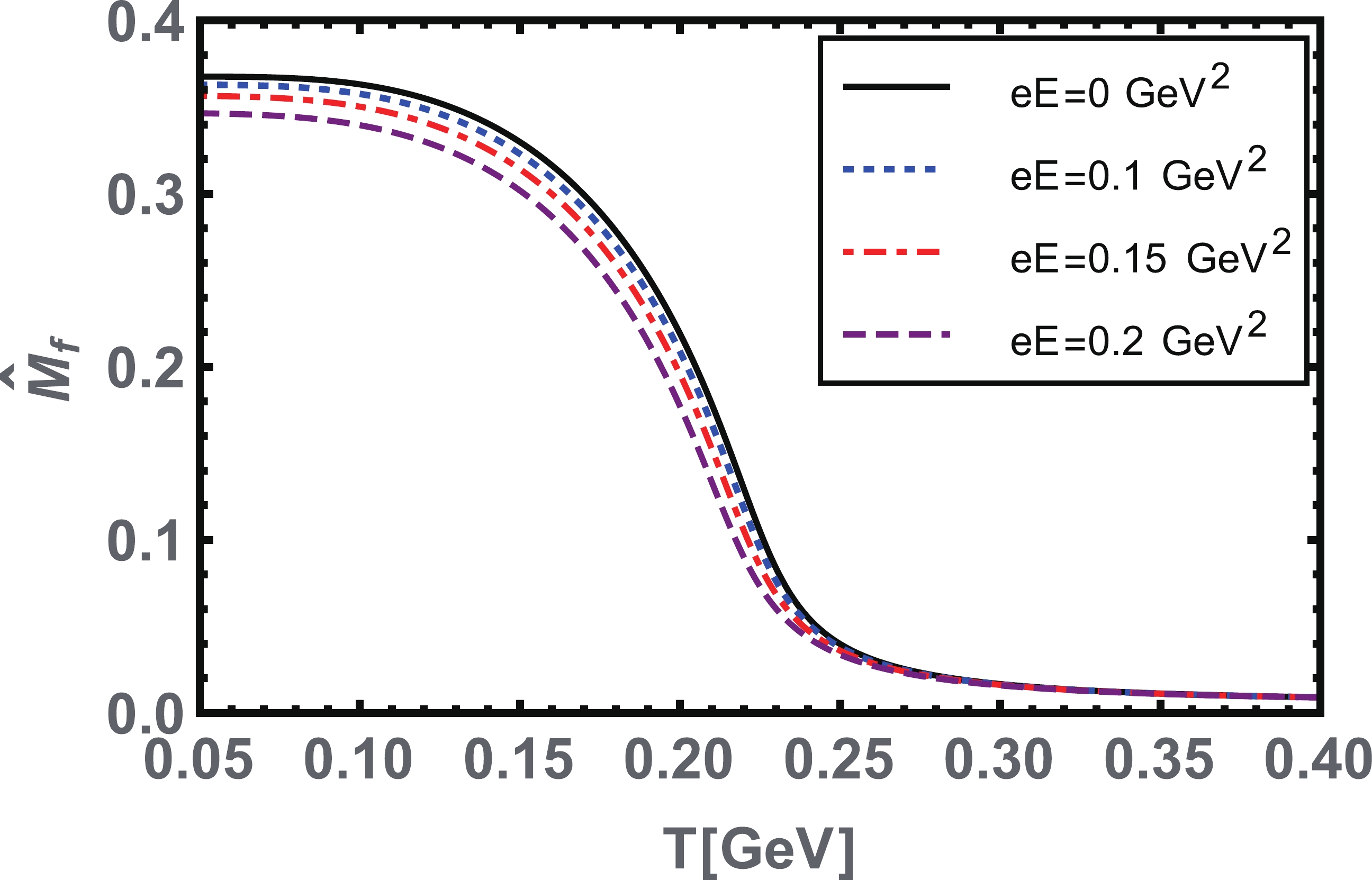
Figure 11.  (color online) Dynamical mass, Eq. (19), as a function of temperature for various given values of electric field strength $eE.$

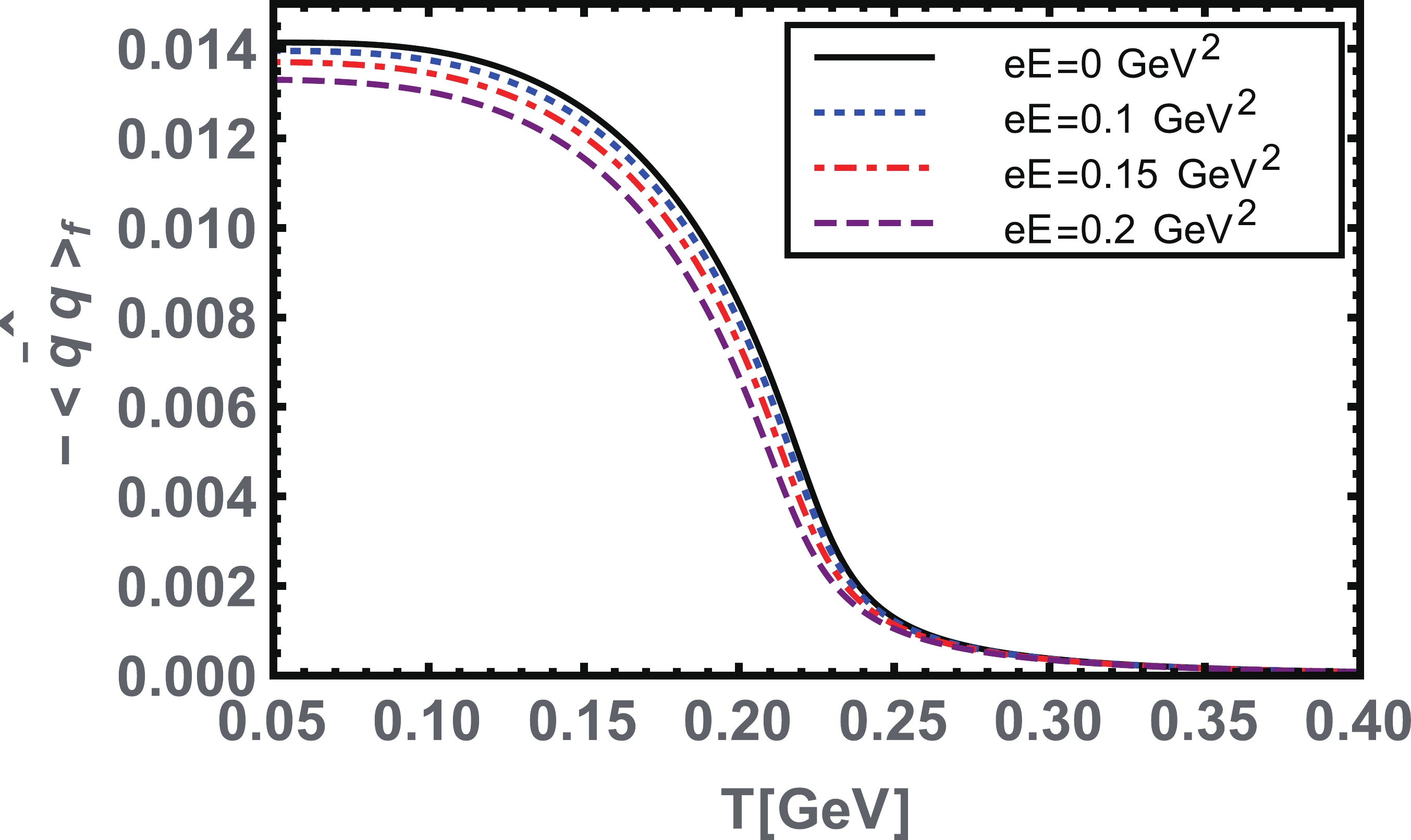
Figure 12.  (color online) Quark-antiquark condensate, Eq. (21), plotted as a function of temperature for various given values of electric field $eE.$

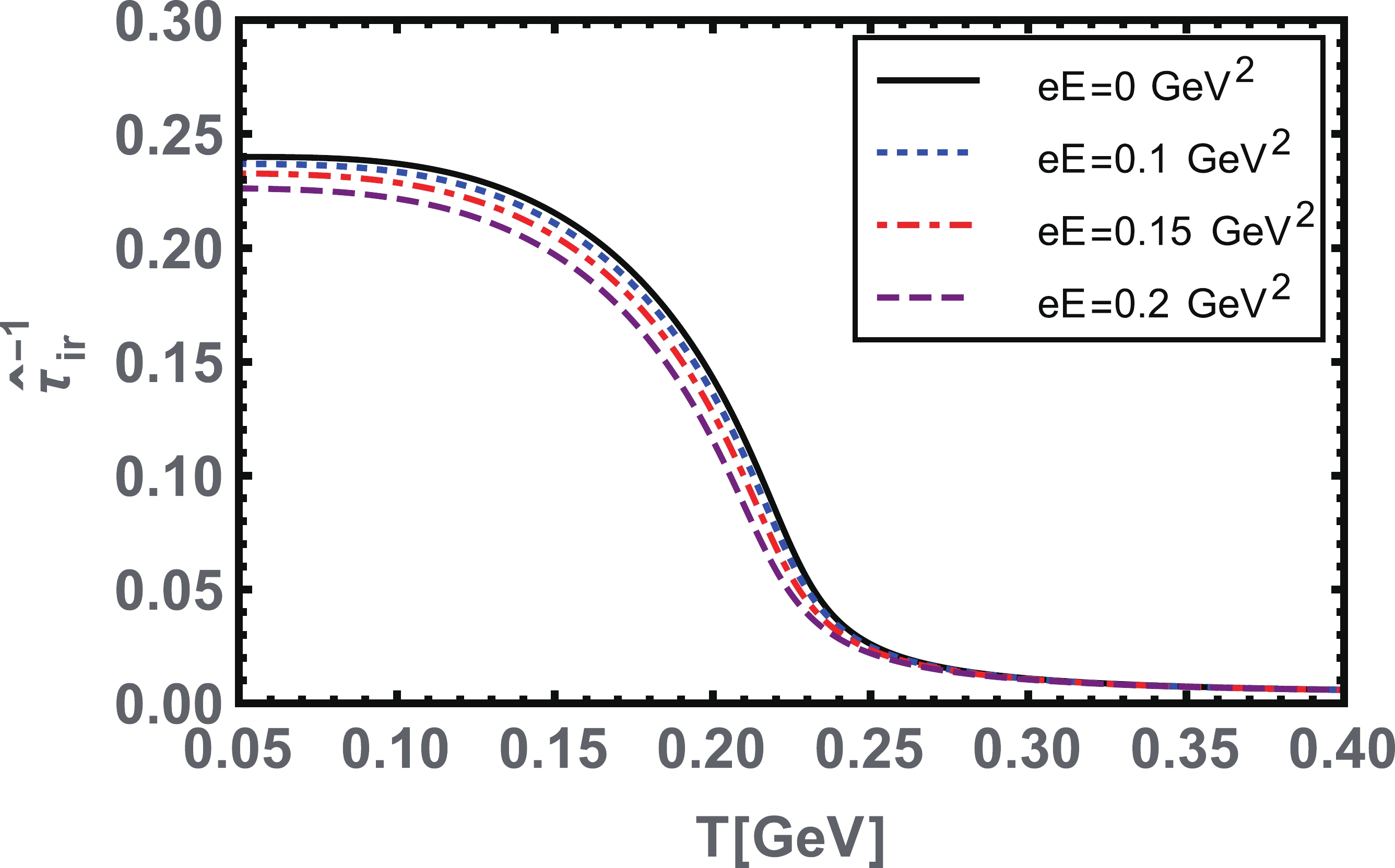
Figure 13.  (color online) Behavior of confinement scale, Eq. (20), plotted as a function of temperature for different given values $eE.$

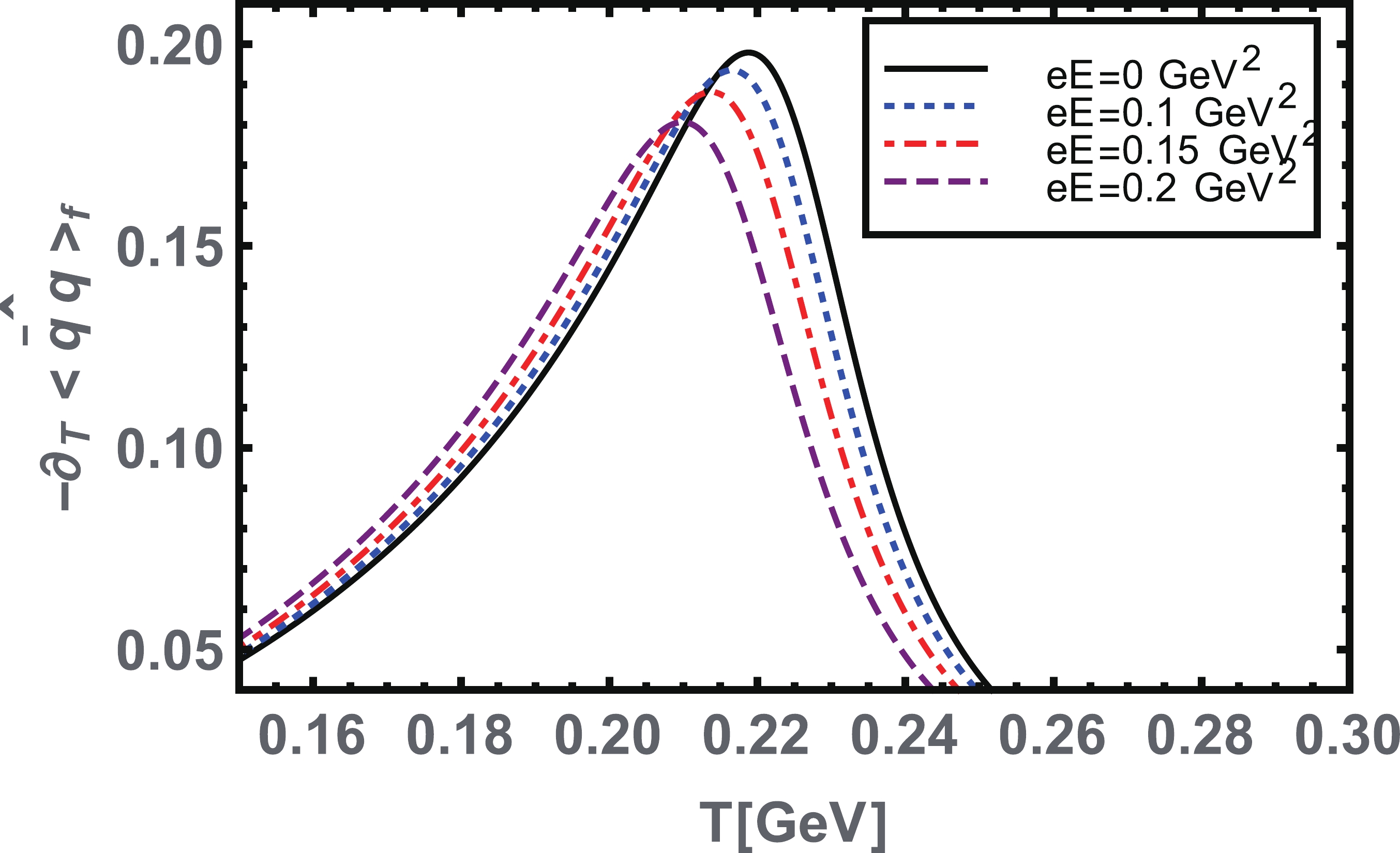
Figure 14.  (color online) Thermal gradient of the quark-antiquark condensate plotted as a function of temperature T for various values of the electric field $eE$. The peaks in the derivatives shift toward low temperature regions from small to large values of $eE.$

Figure 15.  (color online) Thermal gradient of the confinement scale $\partial _{T} \hat{\tau}^{-1}_{ir}$ plotted as a function of temperature T for various values of $eE.$

Second, we consider the case of a pure magnetic field at finite temperature T. We plot the thermal gradient of the quark-antiquark condensate and the confinement length scale, as presented in Figs. 16 and 17, respectively. We note that the inflection points in both parameters shift toward the higher temperatures. In other words, $eB$ enhances the pseudo-critical temperature $T^{\chi, C}_c$ of chiral symmetry restoration and deconfinement. Hence, in a pure magnetic case and at a finite temperature, we observe the magnetic catalysis phenomenon, which has already been observed in the CI model [22, 63].

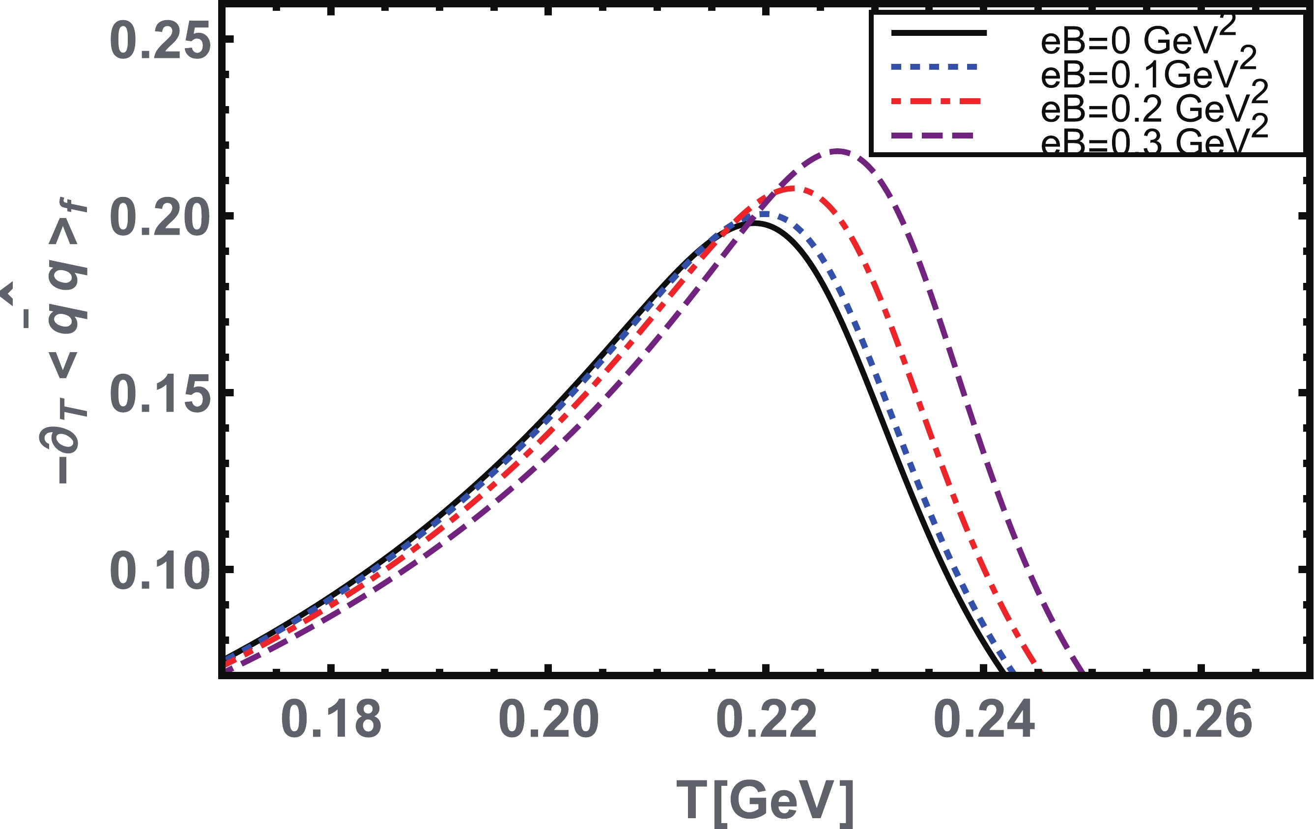
Figure 16.  (color online) Thermal gradient of the quark-antiquark condensate plotted as a function of temperature T for various values of magnetic field $eB$. From the plots, it is evident that the peaks shift toward higher temperatures.

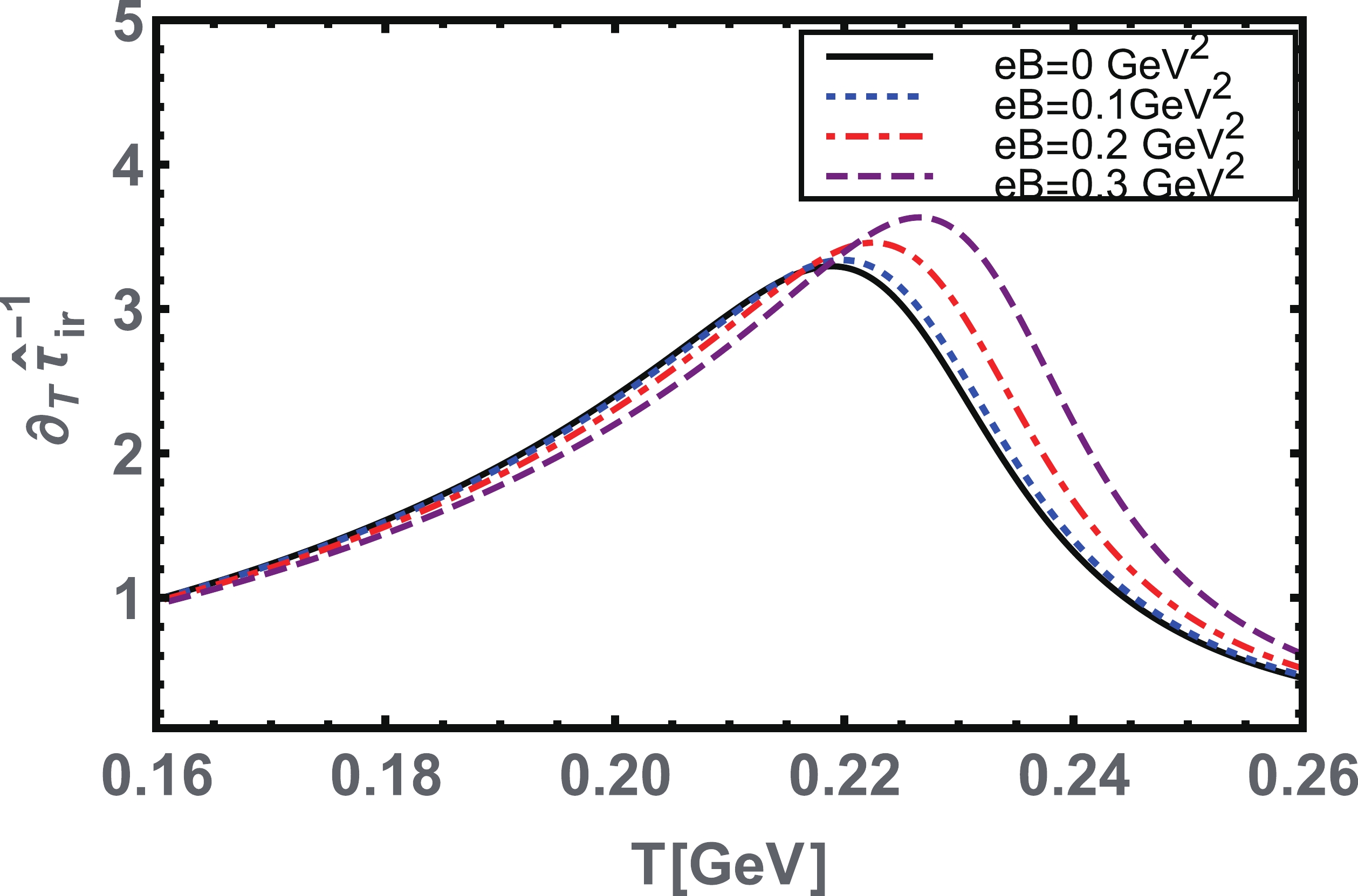
Figure 17.  (color online) Thermal gradient of the confinement scale $\partial _{T}\hat{\tau}^{-1}_{ir}$ plotted as a function of temperature for several values of the magnetic field strength field $eB.$

In most effective model calculations of QCD, it is well demonstrated that to reproduce the inverse magnetic catalysis effect as predicted by the lattice QCD [13, 14], the effective coupling must be taken as magnetic field dependent [17, 22, 28, 63] or both temperature and magnetic field dependent [16, 19, 23, 63, 64]. In the case of this study, we just employed the following functional form of the $eB$-dependent effective coupling ${\rm\alpha_{eff}}(eB)$ [22], where the coupling decreases with the magnetic field strength as

here $\kappa = eB/\Lambda^2_{\rm QCD}$, with $\Lambda_{\rm QCD} = 0.24$ GeV. The parameters a, b, c, and d were extracted to reproduce the behavior of critical temperature $T^{\chi,C}_{c}$ for the chiral symmetry restoration and deconfinement in the presence of magnetic field strength, obtained by lattice QCD simulations [13, 14]. The thermal gradients of the condensate and the confinement length scale, with the magnetic field dependent coupling, Eq. (22), is plotted in Figs. 18 and 19, respectively. It can be observed that the critical $T^{\chi,C}_{c}$ decreases with an increase in $eB$ ; hence, the inverse magnetic catalysis can be observed at a finite T.

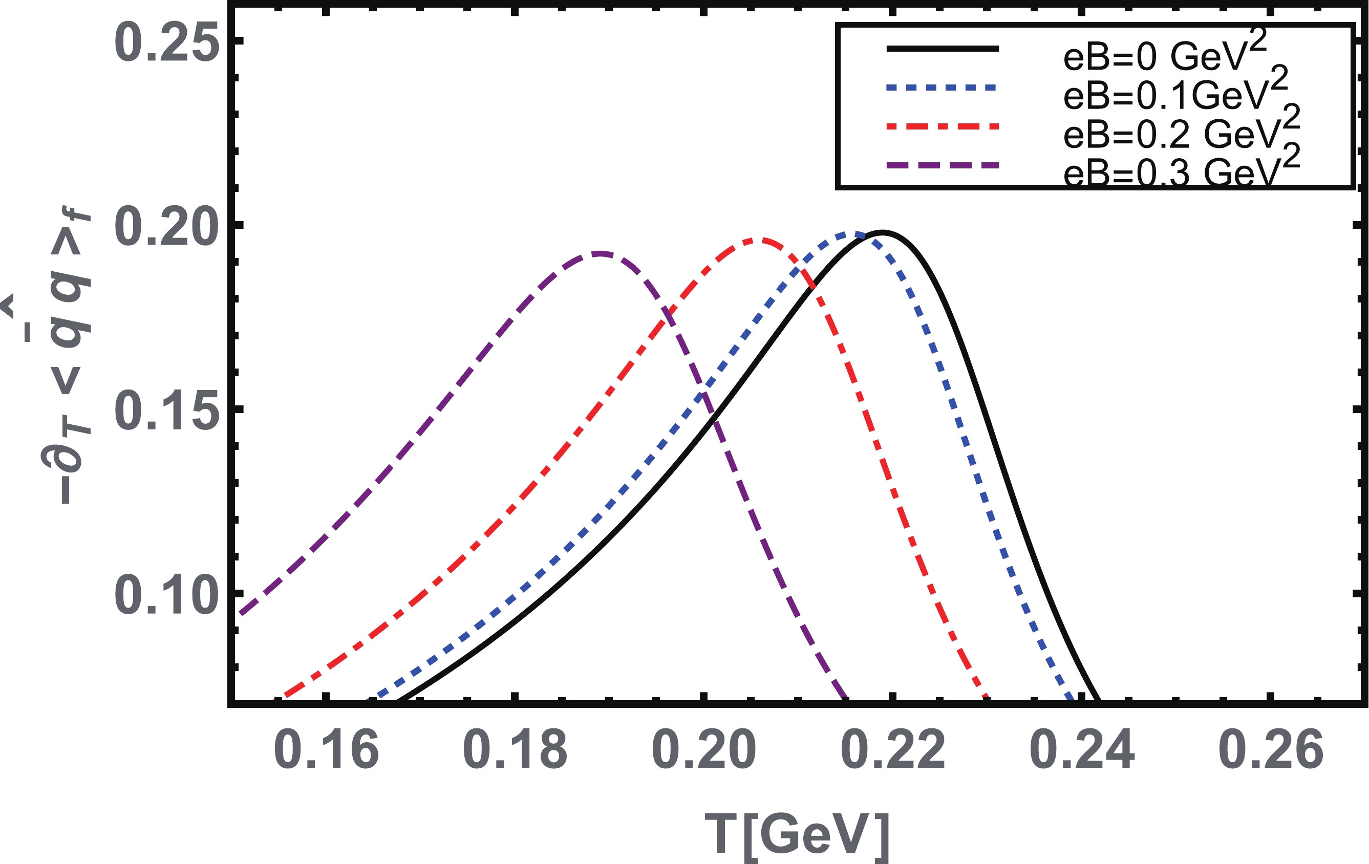
Figure 18.  (color online) Thermal gradient of the condensate with magnetic field dependent coupling, Eq. (22), plotted as a function of temperature for several values of magnetic field strength. The IMC effect is depicted in this figure.

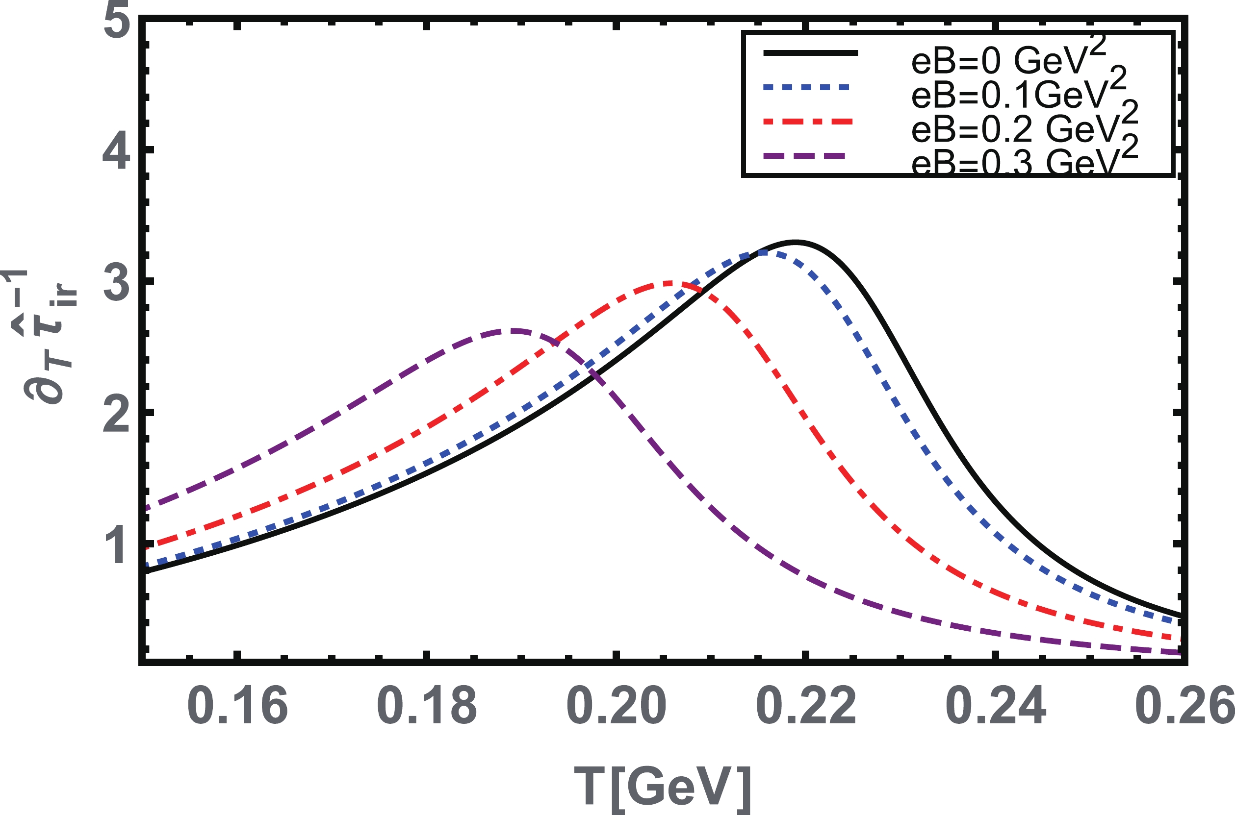
Figure 19.  (color online) Behavior of $\partial _{T}\widehat{\tau}^{-1}_{ir}$ with the magnetic field dependent coupling, Eq. (22), as a function of temperature for several values of magnetic field strength $eB.$

In Fig. 20, we sketch the combined phase diagram in the $T^{\chi,C}_{c}-eE,\;eB$ planes, where we demonstrated the inverse electric catalysis, magnetic catalysis, and inverse magnetic catalysis (with magnetic dependent coupling). In the pure electric background, the solid-black curve indicates that the critical temperature $T^{\chi, C}_{c}$ decreases with an increase in $eE$; hence, the electric field strength inhibits the chiral symmetry breaking and confinement. In the pure magnetic limit (without magnetic field dependent coupling), the magnetic field $eB$ enhances the critical temperature $T^{\chi, C}_{c}$, and thus $eB$ acts as a facilitator of chiral symmetry breaking and confinement. If we use the magnetic field dependent coupling, it can be observed that the critical temperature $T^{\chi, C}_{c}$ decreases as the magnetic field strength $eB$ increases (red dotted-dashed curve). In this case, $eB$ acts as an inhibitor of the chiral symmetry and confinement.

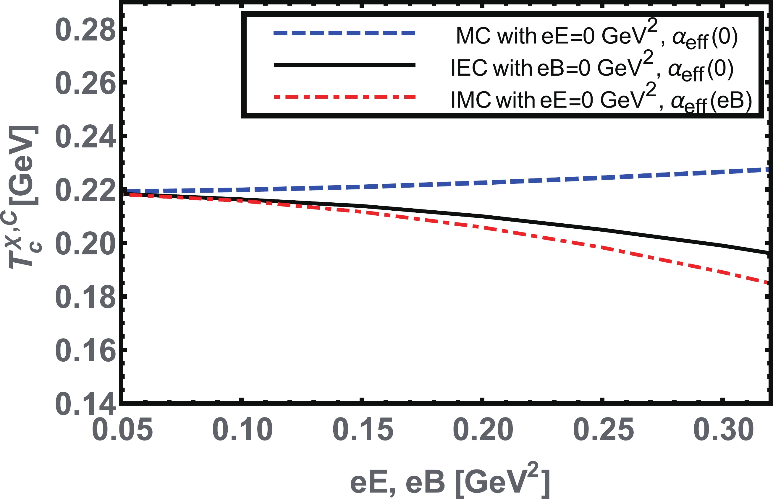
Figure 20.  (color online) Combined phase diagram in the $T^{\chi,C}_{c}$ vs $eE,\;eB$ planes of chiral symmetry breaking and confinement. The plot shows the evalution of IEC as well as MC without and IMC with $eB$-dependent coupling, Eq. (22). The $T^{\chi,C}_{c}$ values are obtained from the inflection points in $\partial _{T}\widehat{\sigma}$ and $\partial _{T}\widehat{\tau}^{-1}_{ir}.$

Third, we adopt both the non-zero values of $eE$ and $eB$ , and draw the phase diagram in the $T^{\chi,C}_{c}-eE$ plane for various given values of $eB$ , as shown in Fig. 21. At this point, the competition between IEC vs MC starts: the $eB$ tends to catalyze the chiral symmetry breaking and confinement; consequently, $T^{\chi, C}_{c}$ is enhanced. In contrast, $eE$ tries to inhibit the chiral phase transition and tends to suppres $T^{\chi, C}_{c}$; finally, it is concluded with a combined inverse electromagnetic catalysis (IEMC). This may be different for a very strong $eB$, where the $eB$ dominates over the $eE$. Next, we consider the $eB$-dependent coupling, Eq. (22), and sketch the phase diagram $T^{\chi,C}_{c}$ vs $eE$ for various given values of $eB$ in Fig. 22. It can be observed that the effect of parallel $eE$ and $eB$ with $eB$-dependent coupling tends to reduce $T^{\chi,C}_{c}$. Therefore, both $eE$ and $eB$ produce IEC and IMC simultaneously.

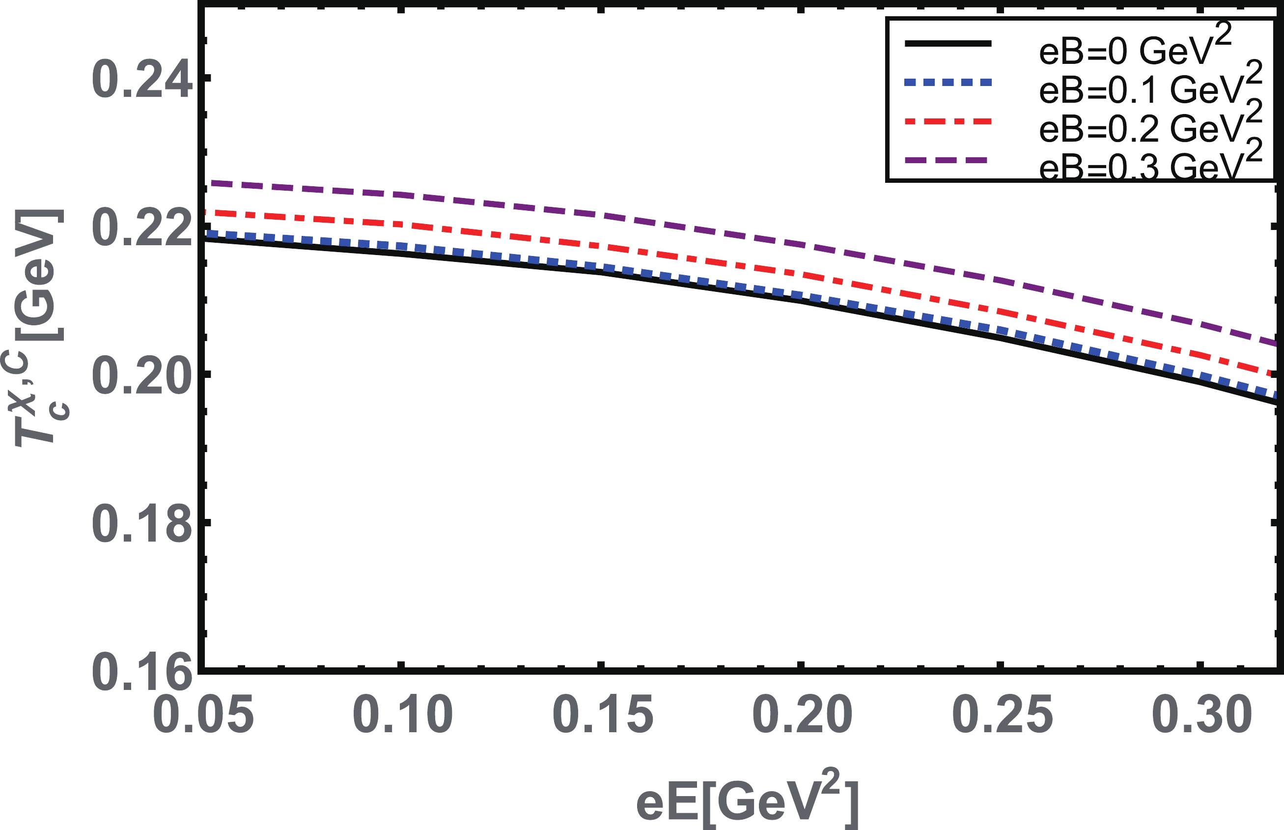
Figure 21.  (color online) Phase diagram in the $T^{\chi, C}_{c}$–$eE$ plane of chiral symmetry breaking and confinement for various given values of $eB$. Here, $eE$ inhibits the chiral phase transition, whereas $eB$ facilitates it; consequently, the IEMC effect is observed.

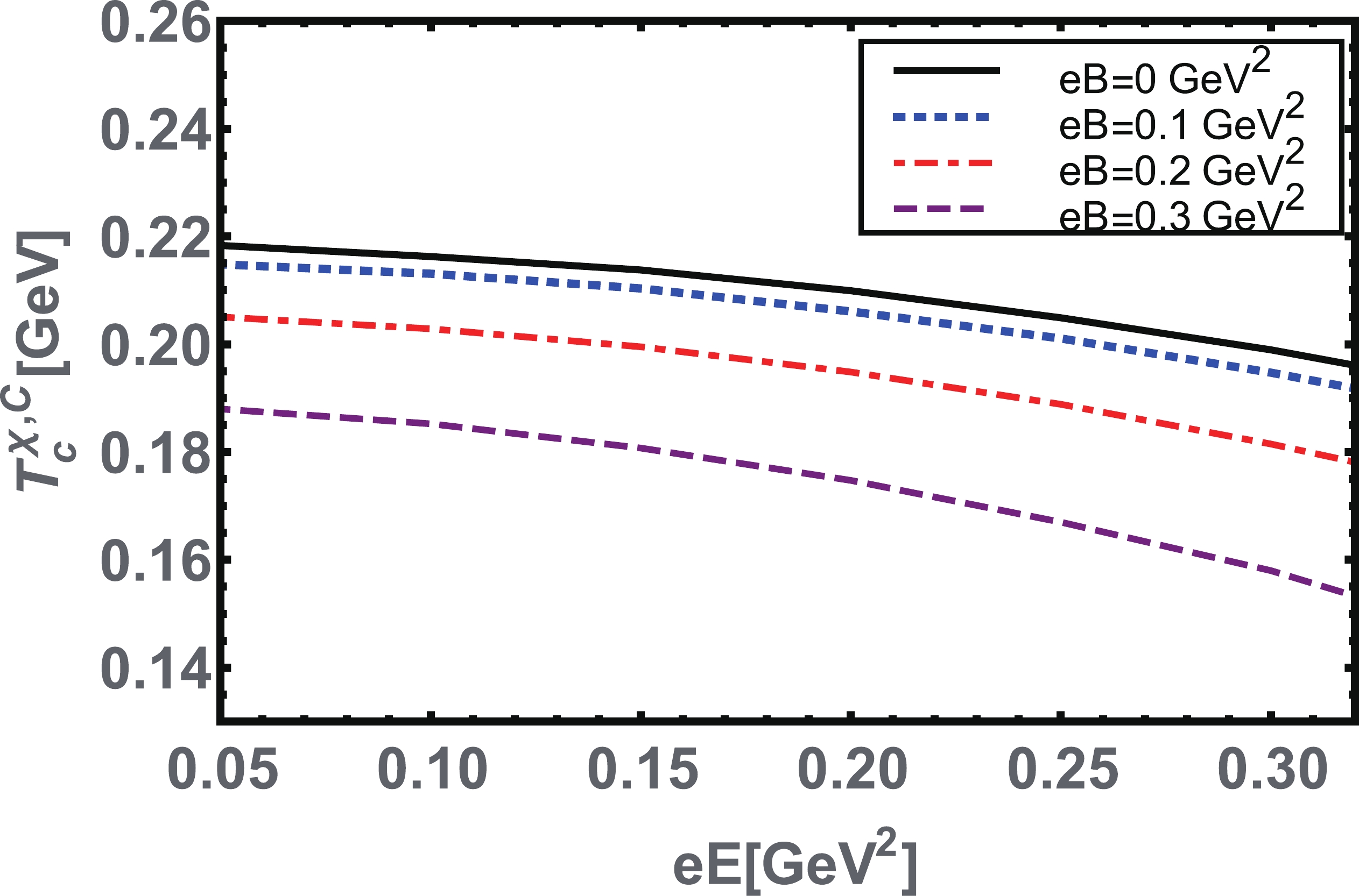
Figure 22.  (color online) Phase diagram in the $T^{\chi,C}_{c}$ vs eE of chiral symmetry breaking and confinement for various given values of eE with eB-dependent coupling Eq. (22). Here, both fields eE and eB inhibit the chiral phase transition; hence, the IEMC is observed.

In this work, we studied the influence of uniform, homogeneous, and external parallel electric and magnetic fields on the chiral phase transitions. In this context, we implemented the Schwinger-Dyson formulation of QCD, with a gap equation kernel comprising a symmetry preserving vector-vector contact interaction model of quarks in a rainbow-ladder truncation. Subsequently, we adopted the well-known Schwinger proper-time regularization procedure. The findings of this study are presented as follows.

At zero temperature, in the pure magnetic background, the magnetic field facilitated the dynamical chiral symmetry breaking and confinement; hence, we observed the magnetic catalysis phenomenon. However, the electric field tends to restore chiral symmetry and deconfinement above the pseudo-critical electric field $eE^{\chi, C}_c\approx0.34$ GeV$^2$, i.e., the chiral rotation effect demonstrated in the proposed model. We observed that the electric field acted as an inhibitor of the chiral symmetry breaking and confinement. When both $eE$ and $eB$ were considered, we determined the magnetic catalysis effect for small given values of $eE$ up to and above the critical electric field strength $eE_{c}\approx0.33$ GeV$^2$, where the other parameters exhibited the de Haas-van Alphen oscillatory type behavior in the region $eB = [0.3-0.54]$ GeV$^2$. In this particular region,$eE$ dominated over $eB$ , and we observed the electric chiral inhibition effect, while above that region where $eB$ was superior to $eE$, we observed magnetic catalysis again. We also realized that the pseudo-critical strength $eE^{\chi, C}_{c}$ was suppressed with the increase in $eB$ , and the transition nature was determined to be the smooth cross-over nature up to and above the pseudo-critical magnetic field strength $eB^{\chi, C}_{c}\approx0.3$ GeV$^2$ , where the transition suddenly changed to the first order transition. Subsequently, we located the position of the critical endpoint at $(eB_p\approx0.3,\;eE_p\approx0.33)$ GeV$^{2}$. We further determined that $eE^{\chi,C}_{c}$ initially remains constant in the limited region $eB = [0.3-0.54]$ GeV$^2$ and then increases with larger values of $eB$.

Finally, we sketched the phase diagram at a finite temperature and in the presence of parallel electric and magnetic fields. At a finite T, in the pure electric field limit, we determined that the pseudo-critical temperature decreased as we increased$eE$; hence, the inverse electric catalysis was observed. However, for the pure magnetic field background, we observed the magnetic catalysis effect in the mean-field approximation and inverse magnetic catalysis with $eB$-dependent coupling. The combined effect of both $eE$ and $eB$ on $T^{\chi, C}_c$ yielded the inverse electromagnetic catalysis, with and without $eB-$dependent effective coupling of the model.

Qualitatively and quantitatively, the predictions of the presented CI-model agree well with results obtained from other effective QCD models, as well as modern Lattice QCD results. In the near future, we plan to extend this work to study the Schwinger pair production rate, including the dynamical chiral symmetry breaking for a higher number of colors, flavors, and in a parallel electromagnetic field. We are also interested in extending this work to study the IEMC phenomenon with the electric field and temperature-dependent coupling. Regarding the dependence of the model coupling on the considered electric field, there is no first-principle simulation for comparisons because lattice simulations in the presence of real electric background fields are not feasible to date. However, progress in this case has commenced, and results will be published somewhere else. The next strategy will be to study the properties of light hadrons in the background of parallel electric and magnetic fields.

The author acknowledges A. Bashir, A. Raya, R.L.S. Farias, and E. V. Gorbar for their valuable suggestions in the process of completing this work. The author also thanks his colleagues at the Institute of Physics, Gomal University, Pakistan.