Radiative decay of the Ξ(1620) in a hadronic molecule picture

I. INTRODUCTION

• I. INTRODUCTION
• II. THEORETICAL FORMALISM
• III. NUMERICAL RESULTS AND DISCUSSIONS
• IV. SUMMARY
• APPENDIX A

Searching for hadrons beyond the constituent quark model is one of the most important topics in the hadron physics community. In the conventional quark model, a hadron is composed of $q\bar{q}$ as a meson or $qqq$ as a baryon. It is natural to expect the existence of hadrons composed of more quarks, which are called exotic states. Because of the significant experimental progress over the past twenty years, more exotic states have been observed [1]. Last year, the $\Xi(1620)$ state, which is cataloged in the Particle Data Group (PDG) [1] with only one star, was reported again in the $\Xi^{-}\pi^{+}$ final state by the Belle Collaboration [2]. The observed resonance parameters of the structure are

which are consistent with the earlier measured values [3, 4]. However, its spin-parity remains undetermined.

From the observed decay model, $\Xi(1620)$ is a conventional baryon composed of $uss$ or $dss$. However, its properties, such as the spectroscopy and decay width, cannot be simply explained in the context of conventional constituent quark models [5-8]. As indicated in Refs. [9-16], $\Xi(1620)$ can be understood as a molecular state in comparison with the Belle data [2]. A molecular state with a narrow width and a mass of approximately 1606 MeV was predicted in the unitarized coupled channels approach [9-12]. However, a $\Xi$ bound state with a mass of approximately 1620 MeV and $J^P = 1/2^{-}$ was predicted by studying the $\bar{K}\Lambda$ interaction in the framework of the one-boson-exchange (OBE) model [15]. Additionally, Ref. [15] considered $\Xi(1620)$ as a pure molecular state composed of $\bar{K}\Lambda$ component. A possible explanation for these results of Refs. [9-12, 15] is that $\Xi$(1620) has a larger $\bar{K}\Lambda$ component [14, 16]. Moreover, the $\bar{K}\Sigma$ component cannot be underestimated to reproduce the total decay width of $\Xi(1620)$ and a study of only the spectroscopy does not provide a complete description of its nature [16].

From the above discussion, $\Xi(1620)$ may be a molecular state. However, currently, we cannot fully exclude other possible explanations such as a mixture of three-quark and five-quark components (as long as quantum numbers permit, this might be the reality). Further research is required to distinguish whether it is a molecular or compact multi-quark state. The photon coupling with a quark is significantly different from the coupling of the photon to the constituent $\bar{K}\Lambda$ and $\bar{K}\Sigma$ of $\Xi(1620)$ [17]. Hence, a precise measurement of the radiative decays is useful to test different interpretations of $\Xi(1620)$. In this paper, we study the radiative decay of $\Xi(1620)$ using the hadronic molecule approach developed in our previous study [16].

The remainder of the paper is organized as follows. The theoretical formalism is explained in Sec. II. The predicted partial decay widths are presented in Sec. III, followed by a short summary in the final section.

II. THEORETICAL FORMALISM

• I. INTRODUCTION
• II. THEORETICAL FORMALISM
• III. NUMERICAL RESULTS AND DISCUSSIONS
• IV. SUMMARY
• APPENDIX A

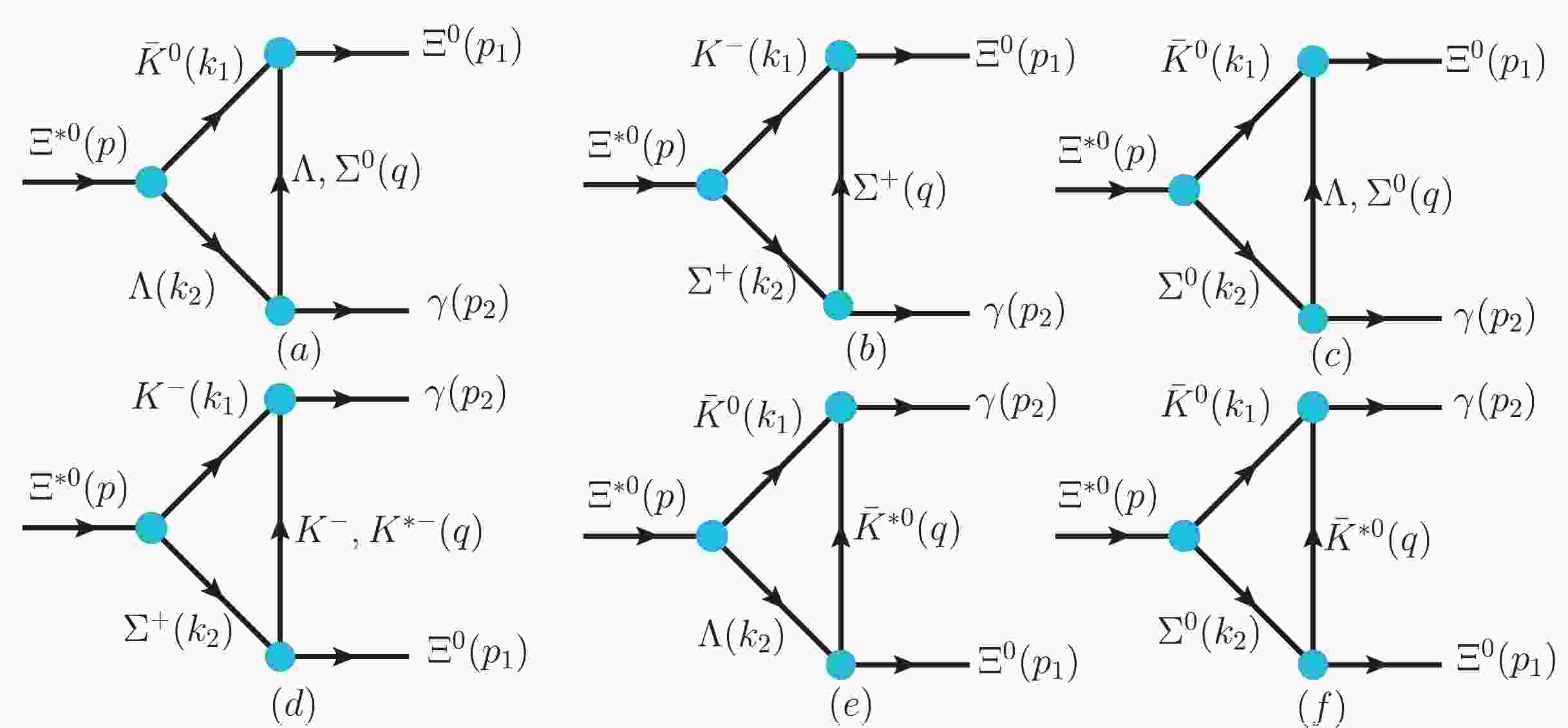
In our previous study [16], the total decay width of $\Xi(1620)$ was reproduced with the assumption that $\Xi(1620)$ is an $S$-wave $\bar{K}\Lambda-\bar{K}\Sigma$ bound state with $J^P = 1/2^{-}$. Based on the molecular scenario, the radiative decay widths $\Xi(1620)\to\gamma\Xi$, $\Xi(1620)\to\gamma\bar{K}\Lambda$, and $\Xi(1620)\to\gamma\pi\Xi$ are studied to elucidate the internal structure of the $\Xi(1620)$ state. To calculate the radiation decay, we first employ the Weinberg compositeness rule to determine $\Xi(1620)$ couplings to its constituents $\bar{K}Y$ ($Y\equiv\Lambda,\Sigma$). Radiative decays occurs from the exchange of a suitable hadron between the $\bar{K}Y$ pair, which then transforms into $\Xi\gamma$,$\gamma\bar{K}\Lambda$, and $\Xi\pi\gamma$. The corresponding Feynman diagrams are shown in Fig. 1 and Fig. 2.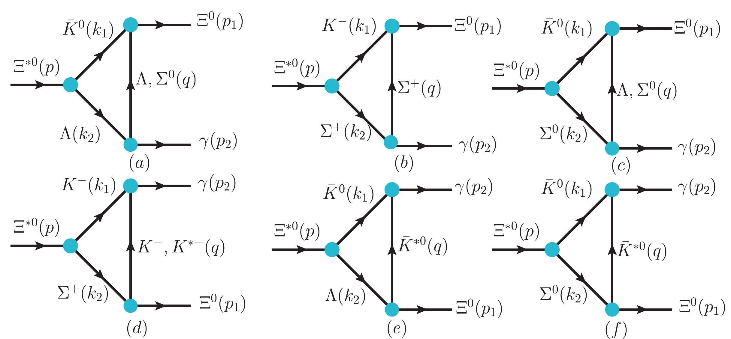

Figure 1

Figure 1.  (color online) Feynman diagrams of the $\Xi^{*0}\to{}\gamma\Xi^{0}$ decay processes. We also indicate the definitions of the kinematics ($p,k_1,k_2,p_1,p_2$, and q) used in the calculation.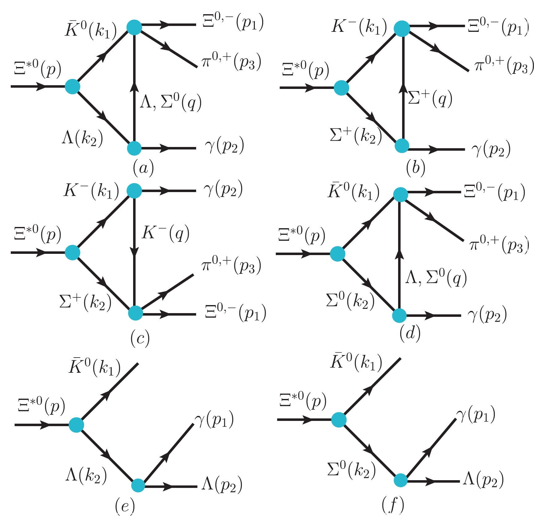

DownLoad: Full-Size Img PowerPoint

Figure 2

Figure 2.  (color online) Feynman diagrams of the $\Xi^{*0}\to$$\gamma\Xi^{0}\pi^0$, $\gamma\Xi^{-}\pi^{+}$, and $\gamma\bar{K}\Lambda$ decay processes. We also indicate the definitions of the kinematics ($p,k_1,k_2,p_1,p_2$,$p_3$, and q) used in the calculation.

DownLoad: Full-Size Img PowerPoint

To compute the diagrams shown in Figs. 1-2, we require the effective Lagrangian densities for the relevant interaction vertices. For the $\Xi(1620)\bar{K}Y$ vertices, the Lagrangian densities can be expressed as [16, 18, 19]

where $\omega_{\bar{K}} = m_{\bar{K}}/(m_{\bar{K}}+m_{Y})$ and $\omega_{Y} = m_{Y}/(m_{\bar{K}}+m_{Y})$. For an isovector baryon $\Sigma$, Y should be replaced with $\vec{Y}\cdot\vec{\tau}$, where $\tau$ is the isospin matrix. $\Phi(y^2)$ is an effective correlation function that is introduced to describe the distribution of the constituents $\bar{K}$ and Y in the hadronic molecular $\Xi(1620)$ state, which is often selected to be of the following form [16, 18-26]:

where $p_E$ is the Euclidean Jacobi momentum and $\beta$ is the size parameter that characterizes the distribution of the components inthe molecule. Currently, the value of $\beta = 1.0$ is determined by experimental data [16, 18-26] (and references therein).

The coupling constant $g_{\Xi(1620)\bar{K}Y}$ is determined by the compositeness condition [16, 18-26], which implies that the renormalization constant of the bound state wave function $\Xi(1620)$ is set to zero

where $x_{AB}$ is the probability of the $\Xi(1620)$ being in the hadronic state $AB$ with normalization $x_{\bar{K}\Sigma}+x_{\bar{K}\Lambda} =$$1.0$. $\Sigma_{\Xi(1620)}$ is the self-energy of the $\Xi(1620)$ and can be computed using the Feynmann diagrams shown in Fig. 3.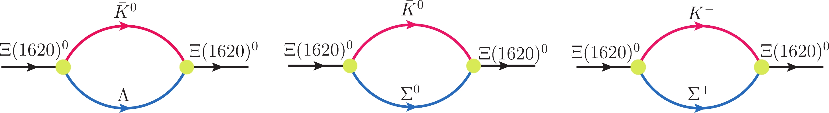

Figure 3

Figure 3.  (color online) Self-energy of the $\Xi$(1620) state.

DownLoad: Full-Size Img PowerPoint

where $z = 2+\alpha+\eta$ and $\Delta = -4\omega_Y-2\eta$. $k_0^2 =$$m^2_{\Xi(1620)}$ with $k_0, m_{\Xi(1620)}$ denoting the four-momenta and mass of the $\Xi(1620)$, respectively; $k_1$, $m_{\bar{K}}$, and $m_{Y}$ are the four-momenta, mass of the $\bar{K}$ meson, and mass of the Y baryon, respectively. Here, we set $m_{\Xi(1620)} = m_{Y}+m_{\bar{K}}-E_b$ with $E_b$ being the binding energy of $\Xi(1620)$. Isospin symmetry implies that

To estimate the radiative decays of the diagrams shown in Figs. 1-2, we require the effective Lagrangian densities related to the photon fields, which are [27, 28]

where the strength tensors are defined as $\sigma_{\mu\nu} =$ $\dfrac{\rm i}{2}(\gamma_{\mu}\gamma_{\nu}-\gamma_{\nu}\gamma_{\mu})$, $F_{\mu\nu} = \partial_{\mu}A_{\nu}-\partial_{\nu}A_{\mu}$, and $K^{*}_{\mu\nu} = \partial_{\mu}K^{*}_{\nu}-$$\partial_{\nu}K^{*}_{\mu}$.$M_N$ is the mass of p, and $\alpha = e^2/4\pi = 1/137$ is the electromagnetic fine structure constant. The anomalous and transition magnetic moments of the baryons are provided by the PDG [1] and are shown in Table 1.

Table 1

Table 1.  Anomalous and transition magnetic moments.

$\kappa_{\Sigma^{-}}=-0.16$	$\kappa_{\Sigma^{0}}=0.65$	$\kappa_{\Sigma^{+}}=1.46$
$\kappa_{\Lambda}=-0.61$	$\mu_{\Sigma\Lambda}=1.61$

DownLoad: CSV

Show Table

The coupling constants $g_{K^{*+}K^{+}\gamma}$ and $g_{K^{*0}K^{0}\gamma}$ are introduced to obtain consistent results with the experimental measurements of $K^{*+}\to{}K^{+}\gamma$ and $K^{*0}\to{}K^{0}\gamma$. The theoretical decay widths of $K^{*+}\to{}K^{+}\gamma$ and $K^{*0}\to{}K^{0}\gamma$ are

According to the experimental widths $\Gamma(K^{*+}\to{}K^{+}\gamma) =$$0.0503$ keV [1] and $\Gamma(K^{*0}\to{}K^{0}\gamma) = 0.125$ keV [1], the coupling constant $g_{K^{*}K\gamma}$ is fixed as

and the signs of these coupling constants are fixed according to the quark model [29, 30].

In addition to the Lagrangians above, the meson-baryon interactions are also required and can be obtained from the following chiral Lagrangians [31, 32]

where $g = 4.64$, $F = 0.51$, $D = 0.75$ [16, 31, 33]; at the lowest order, $u^{\mu} = -\sqrt{2}\partial^{\mu}P/f$ with $f = 93$ MeV;$\langle...\rangle$ denotes the trace in the flavor space; B, P, and $V^{\mu}$ are the $SU(3)$ pseudoscalar meson, vector meson, and baryon octet matrices, respectively, which are

Putting all the pieces together, we obtain the decay amplitudes that are shown in Appendix A. The total amplitudes of the $\Xi^{*0}\to\Xi^{0}\gamma$, $\Xi^{*0}\to\Xi^{0}\pi^0\gamma$, and $\Xi^{*0}\to\pi^{+}\Xi^{-}\gamma$ are the sum of these individual amplitudes, respectively:

When the amplitudes are determined, the corresponding partial decay width can be easily obtained, which is expressed as

The complete explanation of calculating these two equations is available in Refs. [1, 34]. J is the total angular momentum of the $\Xi(1620)$; $|\vec{p}_1|$ is the three-momenta of the decay products in the center of mass frame, and the overline indicates the sum over the polarization vectors of the final hadrons; ($\vec{p}^{*}_3,\Omega^{*}_{p_3}$) is the momentum and angle of the particle $\pi$ in the rest frame of $\pi$ and $\Xi$; $\Omega_{p_2}$ is the angle of the photon in the rest frame of the decaying particle; $m_{13}$ is the invariant mass for $\pi$ and $\Xi$, and $m_{\pi}+m_{\Xi}\leqslant$${}m_{13}\leqslant{}m$.

Using the values obtained above, the radiative decay width of the $\Xi(1620)^0$ into $\Xi^0\gamma$, $\Xi\gamma\pi$, and $\gamma\bar{K}\Lambda$ that are shown in Fig. 1 and Fig. 2 can be calculated. However, the amplitudes of the $\Xi(1620)^0\to\gamma\Xi^0$ and $\Xi(1620)^0\to$$\gamma\Xi\pi$ cannot satisfy the gauge invariance of the photon field. To ensure the gauge invariance of the total amplitudes, the contact diagram must be included. The corresponding Feynman diagrams are shown in Fig. 4. For the this calculation, we adopt the following form to satisfy $p_2^{\mu}{\cal{M}}^{\rm Total}_{\mu}(\equiv{{\cal{M}}}^{T}+{\cal{M}}_{\rm com}) = 0$

Figure 4

Figure 4.  (color online) Contact diagram for $\Xi^{*0}\to\Xi^{0}\gamma$, $\Xi^{*0}\to\Xi^{0}\pi^0\gamma$, and $\Xi^{*0}\to\pi^{+}\Xi^{-}\gamma$. We also indicate definitions of the kinematics ($p_1,p_2,p_3,k_1,k_2$, and p) used in the calculation.

DownLoad: Full-Size Img PowerPoint

where

with $y = 1+\alpha+\eta+\zeta$,${\cal{H}}_2 = 2(\zeta+\omega_{K^{-}})$,${\cal{H}}_1 = 2(\alpha+\omega_{\Sigma^{+}})$, and $m^2_{13} = (p_1+p_3)^2$. m and $m_1$ are the masses of the $\Xi^{*}$ and $\Xi$, respectively.

III. NUMERICAL RESULTS AND DISCUSSIONS

• I. INTRODUCTION
• II. THEORETICAL FORMALISM
• III. NUMERICAL RESULTS AND DISCUSSIONS
• IV. SUMMARY
• APPENDIX A

To compute the radiative decay widths of the considered processes, the coupling constants of $\Xi^{*}(1620)$ to its components can be estimated using the compositeness conditions provided by Eq. (4). $x_{\Lambda\bar{K}}$ in Eq. (4) is the probability of $\Xi(1620)$ being in the hadronic state $\Lambda\bar{K}$. The value of the $x_{\Lambda\bar{K}}$ is in the a range of 0.0-1.0. If $x_{\Lambda\bar{K}}$= 0.0 or 1.0, $\Xi(1620)$ is a pure molecular state containing the components $\Sigma\bar{K}$ and $\Lambda\bar{K}$, respectively. Otherwise $\Xi(1620)$ is a $\bar{K}\Lambda$-$\bar{K}\Sigma$ molecular state. Currently, the value of $x_{\Lambda\bar{K}}$ cannot be accurately determined from first principles; therefore, it should better be determined using experimental data. As the free parameter, $x_{\Lambda\bar{K}} = 0.52-0.68$ is fixed by fitting the experimental decay data on possible $\bar{K}\Lambda$-$\bar{K}\Sigma$ bound states within the same theoretical framework adopted in Ref. [16]. In this region, the total decay width for this state is predicted to be approximately $50.39-68.79$ MeV, which is comparable with the experimental data [2].

Considering $\Xi^{*}(1620)$ loosely as an S-wave $\bar{K}\Lambda$-$\bar{K}\Sigma$ hadronic molecule, the coupling constants $g_{\Xi^{*}(1620)\bar{K}\Lambda}$ and $g_{\Xi^{*}(1620)\bar{K}\Sigma}$ that are dependent on the parameter $x_{\bar{K}\Lambda}$ are plotted in Fig. 5. We observe that the coupling constant $g_{\Xi^{*}(1620)\bar{K}\Lambda}$ monotonously increases with increasing $x_{\bar{K}\Lambda}$ in our considered $x_{\bar{K}\Lambda}$ range, while the coupling constant $g_{\Xi^{*}(1620)\bar{K}\Sigma}$ decreases with increasing $x_{\bar{K}\Lambda}$. The opposite trend can be easily understood, as the coupling constants $g_{\Xi^{*}(1620)\bar{K}\Lambda}$ and $g_{\Xi^{*}(1620)\bar{K}\Sigma}$ are directly proportional to the corresponding molecular compositions [23].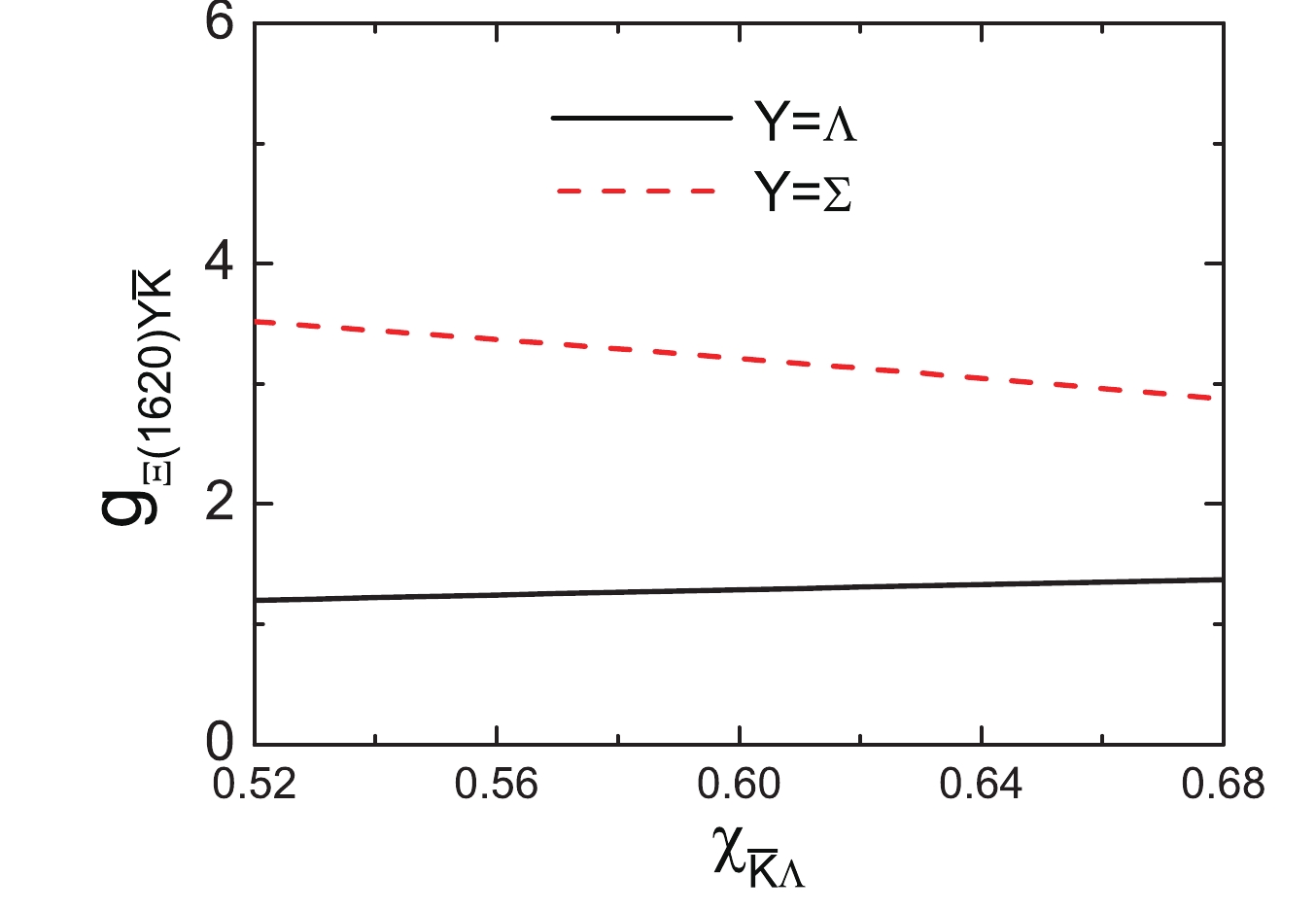

Figure 5

Figure 5.  (color online) $x_{\bar{K}\Lambda}$ dependence of $g_{\Xi^{*}(1620)\bar{K}\Lambda}$ and $g_{\Xi^{*}(1620)\bar{K}\Sigma}$.

DownLoad: Full-Size Img PowerPoint

With the obtained total amplitude, the radiative decay width of $\Xi(1620)^0$ into $\Xi^0\gamma$ can be calculated. The dependence of the corresponding radiative decay width on $x_{\bar{K}\Lambda}$ is depicted in Fig. 6. For the $x_{\bar{K}\Lambda}$ value within a reasonable range from 0.52 to 0.68, the radiative decay width of the $\Xi(1620)^0\to\gamma\Xi^0$ contribution from the $\bar{K}\Sigma$ channel monotonously decreases. However, it increases for the $\bar{K}\Lambda$ channel contribution to the $\Xi(1620)^0\to\gamma\Xi^0$. Moreover, the $\bar{K}\Sigma$ component provides the dominant contribution to the partial decay width of the $\gamma\Xi^0$ two-body channel. The $\bar{K}\Lambda$ contribution to the $\gamma\Xi^0$ two-body channel is very small. This is different from our results in Ref. [16] in that the $\bar{K}\Lambda$ component provides the dominant contribution to the strong decay width of the $\Xi(1620)$. A possible explanation for this may be that the interaction between the $\Sigma$ baryon and photon is stronger than the $\gamma{}-\Lambda$ interaction since the $\Sigma^0$ decays completely to the final state containing the $\Lambda$ baryon and $\gamma$ [1].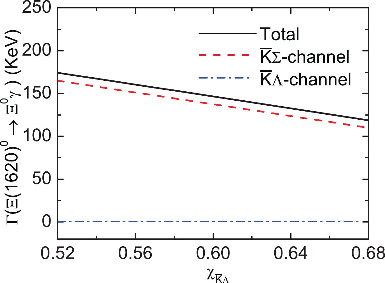

Figure 6

Figure 6.  (color online) Decomposed contributions to the decay width of the $\Xi(1620)^0$ into $\Xi^0\gamma$.

DownLoad: Full-Size Img PowerPoint

Figure 6 also indicates that the total radiative decay width decreases for $\Xi(1620)^0\to\gamma\Xi^0$ when $x_{\bar{K}\Lambda}$ is changed from 0.52 to 0.68. We also observe that the interference between the $\bar{K}\Sigma$ and $\bar{K}\Lambda$ channels is considerably small, resulting in a total decay width of $\Xi(1620)^0\to\gamma\Xi^0$ being primarily contributed by the $\bar{K}\Sigma$ channel. This does not alter the conclusion that the $\bar{K}\Lambda$ channel strongly couples to the $\bar{K}\Sigma$ channel [9, 16]. The main reason for this is that the radiative decay widths are often in the keV regime and are significantly lower than their strong counterparts. Indeed, the total radiative decay width for $\Xi(1620)^0\to\gamma\Xi^0$ is predicted to be $118.76-174.21$ KeV, which is significantly lower than the total decay width, which is predicted to be approximately 50.39-68.79 MeV [16].

The individual contributions of $K^{-}$, $\bar{K}^{*}$, $\Sigma$, $\Lambda$ exchanges, and contact term for the reaction $\Xi(1620)^0\to$$\gamma\Xi^0$ are shown in Fig. 7. The amplitudes corresponding to the $K^{-}$-exchange and $\Sigma^{+}$-exchange are not gauge invariant, while the remainder are gauge invariant. We can observe that the contract term and $K^{-}$-exchange provide a dominant contribution to the total decay width, and is at last sixty orders of magnitude larger than those of the amplitudes corresponding to the $\bar{K}^{*}$, $\Sigma$, and $\Lambda$ exchanges for the studied $x_{\bar{K}\Lambda}$ range.

Figure 7

Figure 7.  (color online) Partial decay widths from $K^{-}$(red dash line), $\bar{K}^{*}$(cyan dash dot line), $\Sigma$ (blue dot line), $\Lambda$(magenta dash dot dot line), and the remainder is the contact term exchange contribution for the $\Xi(1620)^0\to\gamma\Xi^0$ as a function of the parameter $x_{\bar{K}\Lambda}$.

DownLoad: Full-Size Img PowerPoint

Next, we examine the three-body radiative decays $\Xi(1620)^0\to\gamma\pi\Xi$ and $\Xi(1620)^0\to\gamma\bar{K}\Lambda$. The decay widths with $x_{\bar{K}\Lambda}$ varying from 0.52 to 0.68 for such two transitions are depicted in Fig. 8. Since the phase space is small compared with the two-body radiative decay channel $\Xi(1620)^0\to\gamma\Xi^0$, the decay width should be the smallest for the $\Xi(1620)^0\to\gamma\bar{K}\Lambda$ channel, should be intermediate for the $\Xi(1620)^0\to\gamma\pi\Xi$ channel, and the largest for the $\Xi(1620)^0\to\gamma\Xi^0$ channel. Indeed, our study shows that the partial width of $\Xi(1620)^0\to\gamma\bar{K}\Lambda$ is rather small, weakly increasing as $x_{\bar{K}\Lambda}$ increases. In particular, the partial width varies from 0.016 to 0.020 eV in the studied $x_{\bar{K}\Lambda}$ range. However, the partial width of $\Xi(1620)^0\to\gamma\Xi\pi$ decreases as $x_{\bar{K}\Lambda}$ increases, and the partial width of the $\Xi(1620)^0\to\gamma\Xi\pi$ is estimated to be $68.75-58.19$ eV.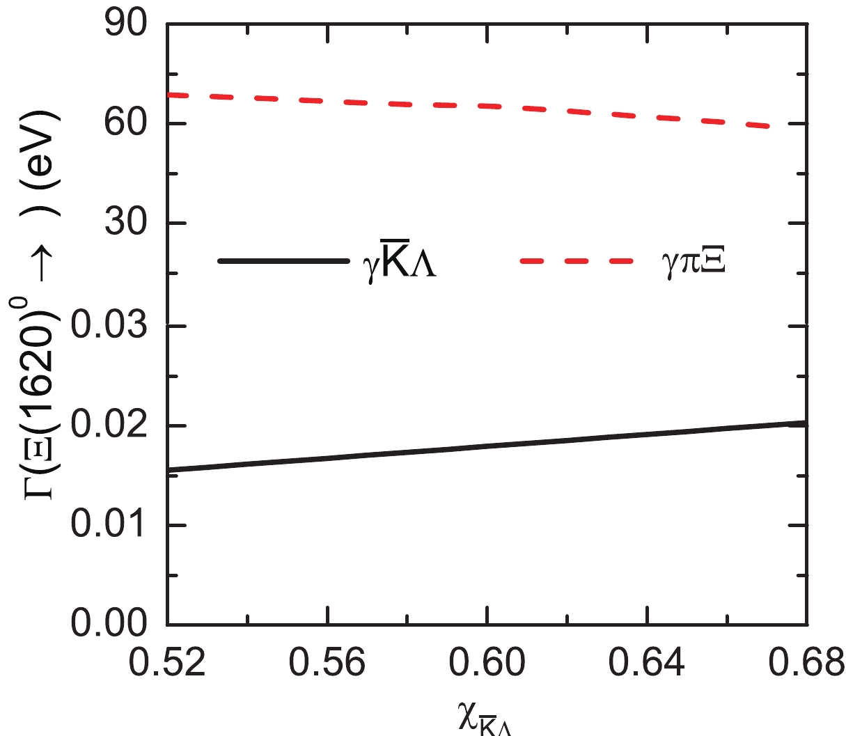

Figure 8

Figure 8.  (color online) Partial decay widths of the $\Xi(1620)^0\to\gamma\Xi\pi$ and $\Xi(1620)^0\to\gamma\bar{K}\Lambda$.

DownLoad: Full-Size Img PowerPoint

In Fig. 2, the diagrams with pion emitted directly from the intermediated $\Lambda$ and $\Sigma$ should be included. Our estimations indicate that in the discussed parameter range, the radiative transition strength for these diagrams are considerably small and the decay width is of the order of approximately 0.1 eV. Moreover, the interferences among them are also rather small. Therefore, the contributions from these channels are not considered in this paper.

IV. SUMMARY

• I. INTRODUCTION
• II. THEORETICAL FORMALISM
• III. NUMERICAL RESULTS AND DISCUSSIONS
• IV. SUMMARY
• APPENDIX A

We have studied the two-body and three-body radiative decays of the $\Xi(1620)$ state assuming that it is a bound state of $\bar{K}\Lambda$-$\bar{K}\Sigma$. The coupling of $\Xi(1620)$ to its components are fixed according to the Weinberg compositeness condition. The radiative decays for $\Xi(1620)^0\to\gamma\Xi^0$ and $\Xi(1620)^0\to\gamma\pi\Xi$ are obtained via triangle diagrams with exchanges of a pseudoscalar meson K, vector meson $K^{*}$, and baryons $\Sigma$ and $\Lambda$. The three-body decay for the $\Xi(1620)^0\to\gamma\bar{K}\Lambda$ occur at the tree level. In the relevant parameter region, the partial widths are evaluated as

Our calculation indicates the partial widths for $\Xi(1620)^0\to\gamma\pi\Xi$ and $\Xi(1620)^0\to\gamma\bar{K}\Lambda$ are too small to be observed, while for $\Xi(1620)^0\to\gamma\Xi^0$, the partial width can reach up to 174 keV at $E_{\rm c.m.} = 1.620$ GeV. Experimentally, with the current integrated luminosity that the LHCb experiment has accumulated at $1.620$ GeV, the process $\Xi(1620)^0\to$$\gamma\Xi^0$ may be searched with only $\gamma\Xi^0$ identified. Such research can also be conducted in the forthcoming Belle II experiment.

APPENDIX A

• I. INTRODUCTION
• II. THEORETICAL FORMALISM
• III. NUMERICAL RESULTS AND DISCUSSIONS
• IV. SUMMARY
• APPENDIX A

Using the Lagrangians in Section II, the amplitudes for the diagrams shown in Figs. 1-2 can be easily obtained:

where $\{{\cal{A}}$, and ${\cal{B}}\}$ are $\Lambda$ and $\Sigma$ baryon exchanges, respectively. The amplitudes of the $\Xi^{0}(1620)\to\gamma\pi\Xi,\gamma\bar{K}\Lambda$ can be also easily obtained:

where the expressions in the curly brackets, $\left \{ \begin{array}{ll} A\\ B \\ \end{array} \right.$, are for $\Xi^{*0}\to\pi^0\Xi^{0}\gamma$ and $\Xi^{*0}\to\pi^{+}\Xi^{-}\gamma$, respectively.

References