


 Abstract
 HTML
HTML Reference
 Related
 PDF
PDF


-
Doubly heavy baryons composed of two heavy quarks and a single light quark are interesting objects. Their investigation can help us better understand the non-perturbative nature of QCD and set up a good framework for understanding and predicting the spectrum of heavy baryons. Moreover, theoretical studies on different aspects of these baryons may shed light on the experimental searches for their states. These baryons have been in the focus of various theoretical studies [1-32]. Some interesting progress on OPE calculations of their lifetimes can be found in [33, 34]. Despite their predictions decades ago via quark model, we have very limited experimental knowledge on these baryons. Nevertheless, 2017 was a special year in this regard, because it was marked by the discovery of the doubly charmed
$ \Xi^{++}_{cc} $ baryon by the LHCb Collaboration [35]. This state was then confirmed in the decay channel$ \Xi^{++}_{cc}\rightarrow \Xi^+_c \pi^+ $ [36]. Although the charmed-bottom state$ \Xi^0_{bc} $ has been searched in the$ \Xi^0_{bc}\rightarrow D^0 p K^- $ decay by the LHCb collaboration, no evidence for a signal has been found [37]. However, the detection of$ \Xi^{++}_{cc} $ has raised hopes for the discovery of other members of doubly heavy baryons. It is remarkable that the LHC is opening new horizons in the discovery of heavy baryons, thus enabling the investigation of their electromagnetic, weak, and strong decays.Beyond the quark models [38-40], many effective models such as lattice QCD [41], Quark Spin Symmetry [42, 43], QCD Sum Rules [22-26], and Light-Cone Sum Rules [19, 20, 44-51] have been proposed to describe masses, residues, lifetimes, strong coupling constants, and other properties of doubly heavy baryons. Given that the expectations to discover more doubly heavy baryons are growing, we are witnessing the rise of further theoretical investigations in this respect.
Concerning the strong decays of doubly heavy baryons, the strong coupling constants are building blocks. They are introduced in the amplitudes of the strong decays, and the widths of the related decays are calculated in terms of these constants. They can also be used to construct the strong potential energy among the hadronic multiplets. These couplings appear in the low-energy (long-distance) region of QCD, where the running coupling becomes larger and the perturbation theory breaks down. Therefore, to calculate such coupling constants, a non-perturbative approach should be used. One of the comprehensive and reliable methods for evaluating non-perturbative effects is the light-cone QCD sum rule (LCSR), which has provided many successful descriptions of the hadronic properties so far. This method is a developed version of the standard technique of SVZ sum rule [52], using the conventional distribution amplitudes (DAs) of the on-sell states. The main difference between the SVZ sum rule and LCSR is that the latter employs the operator product expansion (OPE) near the light-cone
$ x^2\approx 0 $ instead of short distance$ x\approx 0 $ , and the corresponding matrix elements are parametrized in terms of hadronic DAs, which are classified according to their twists [53-55].In this study, we derive the strong coupling constants among the doubly heavy spin-3/2 baryons,
$ \Xi^*_{QQ'} $ and$ \Omega^*_{QQ'} $ , and light pseudoscalar mesons π, K, and η. Here both Q and$ Q' $ can be b or c quarks. The paper is organized as follows. In the next section, we derive the sum rules for the strong coupling constants using the LCSR. Numerical analysis and results are presented in Sec. III. Finally, Sec. IV is devoted to the summary and conclusion. -
In this section, we aim to derive the sum rules for the strong coupling constants among the doubly heavy spin-3/2 baryons (
$ \Xi^{*}_{QQ'} $ and$ \Omega^{*}_{QQ'} $ ) and light pseudoscalar mesons (π, K, and η) using the method of LCSR. The quark content of the doubly heavy spin-3/2 baryons is presented in Table 1.Baryon q Q $ Q^\prime $ 

$ \Xi^*_{QQ^\prime } $ 

u or d b or c b or c $ \Omega^*_{QQ^\prime} $ 

s b or c b or c Table 1. Quark content of the doubly heavy spin-3/2 baryons.
The first step to calculate the strong couplings is to write the proper correlation function (CF) in terms of doubly heavy baryons' interpolating current,
$ \eta_{\mu} $ . That is,$ \Pi_{\mu \nu}(p,q) = {\rm i} \int {\rm d}^4x {\rm e}^{{\rm i}px} \left< {\cal{P}}(q) \vert {\cal{T}} \left\{ \eta_{\mu} (x) \bar{\eta}_{\nu} (0) \right\} \vert 0 \right>, $

(1) where
$ {\cal{P}}(q) $ represents the pseudoscalar meson carrying the four-momentum q, and p represents the outgoing doubly heavy baryon four-momentum. The above CF can be calculated in two ways:$ \bullet $ By inserting the complete set of hadronic states with the same quantum numbers of the corresponding doubly heavy baryons. This is called the physical or phenomenological side of the CF. It is calculated in the timelike region and contains observables such as strong coupling constants.$ \bullet $ By calculating in the deep Euclidean spacelike region with the help of OPE and in terms of DAs of the on-shell mesons and other QCD degrees of freedom. This is called the theoretical or QCD side of the CF.These two sides are matched via a dispersion integral that leads to the sum rules for the corresponding coupling constants. To suppress the contributions of the higher states and continuum, Borel transformation and continuum subtraction procedures are applied. Next, we explain each of these steps in detail.
-
The procedure to construct the doubly heavy spin-3/2 interpolating current is to create a diquark structure with spin one and then attach the remaining spin-1/2 quark to build a spin-3/2 structure, which has to contain the quantum numbers of the related baryon. According to the results reported in [23] and [47], the corresponding interpolating current can be found as follows. The diquark structure has the form
$ \eta_{\text{diquark}} = q_1^T C \Gamma q_2, $

(2) where T and C represent the transposition and charge conjugation operators, respectively, and
$ \Gamma = I, \gamma_5, \gamma_{\mu}, \gamma_{\mu}\gamma_5, $ $ \sigma_{\mu\nu} $ . The dependence of the spinors on the spacetime x is omitted for now. Attaching the third quark, the general form of the corresponding structure is$ \big[q_1^T C \Gamma q_2\big]\Gamma' q_3 $ . Considering the color indices (a,b and c), the possible structures have the following forms:$ \varepsilon_{abc}(Q^{aT} C \Gamma Q^{'b})\Gamma' q^c $ ,$ \varepsilon_{abc}(q^{aT} C \Gamma Q^{b})\Gamma' Q^{'c} $ , and$ \varepsilon_{abc}(q^{aT} C \Gamma Q^{'b})\Gamma' Q^{c} $ , where$ Q^{(')} $ and q are the heavy and light quark spinors respectively and the antisymmetric Levi-Civita tensor,$ \varepsilon_{abc} $ , makes the interpolating current color singlet.The Γ matrices can be determined by investigating the diquark part of the interpolating current. In the first form, as the diquark structure has spin 1, it must be symmetric under the exchange of the heavy quarks
$ Q \leftrightarrow Q' $ . Transposing yields to$ \begin{aligned}[b] \Big[\epsilon_{abc} Q^{aT} C\Gamma Q'^b \Big]^T = &-\epsilon_{abc} Q'^{bT} \Gamma^T C^{-1} Q^a\\ =& \epsilon_{abc} Q'^{bT} C(C\Gamma^T C^{-1}) Q^a, \end{aligned} $

(3) where we have used the identities
$ C^T = C^{-1} $ and$ C^2 = -1 $ , and consider the anticommutation of the spinor components because they are Grassmann numbers. Given that$ C = i \gamma_2 \gamma_0 $ , the quantity$ C\Gamma^T C^{-1} $ would be$ C{\Gamma ^T}{C^{ - 1}} = \left\{ {\begin{array}{*{20}{l}} \Gamma &{{\rm{for}}\;\Gamma = 1,{\gamma _5},{\gamma _\mu }{\gamma _5},}\\ { - \Gamma }&{{\rm{for}}\;\Gamma = {\gamma _\mu },{\sigma _{\mu \nu }}.} \end{array}} \right. $

(4) Therefore, after switching the dummy indices in the LHS of Eq. (3), we obtain
$ \Big[\epsilon_{abc} Q^{aT} C\Gamma Q'^b \Big]^T = \pm \epsilon_{abc} Q'^{aT} C\Gamma Q^b, $

(5) where the
$ + $ and$ - $ signs are for$ \Gamma = \gamma_{\mu}, \sigma_{\mu \nu} $ and$ \Gamma = 1, $ $ \gamma_5, \gamma_5\gamma_\mu $ , respectively. Moreover, given that the RHS of the above equation has to be symmetric with respect to the exchange of heavy quarks, we have$ \Big[\epsilon_{abc} Q^{aT} C\Gamma Q'^b \Big]^T = \pm \epsilon_{abc} Q^{aT} C\Gamma Q'^b, $

(6) where the
$ + $ and$ - $ signs are for$ \Gamma = \gamma_{\mu}, \sigma_{\mu \nu} $ and$ \Gamma = 1, \gamma_5, $ $ \gamma_5\gamma_\mu $ respectively. Moreover, we know that the structure$ \epsilon_{abc} Q^{aT} C\Gamma Q'^b $ is a number ($ 1 \times 1 $ matrix), and therefore, the transposition leaves it unchanged. This leads us to conclude that the only possible choice for the Γ matrices would be$ \Gamma = \gamma_{\mu} $ or$ \sigma_{\mu \nu} $ .The aforementioned symmetry of exchanging heavy quarks should be properly respected by the two remaining structures, i.e.,
$ \varepsilon_{abc}(q^{aT} C \Gamma Q^{b})\Gamma' Q^{'c} $ and$ \varepsilon_{abc}(q^{aT} C \Gamma Q^{'b})\Gamma' Q^{c} $ , which leads to the following form:$ \varepsilon_{abc}\big[(q^{aT} C \Gamma Q^{b})\Gamma' Q^{'c} + (q^{aT} C \Gamma Q^{'b})\Gamma' Q^{c}\big], $

(7) where
$ \Gamma = \gamma_{\mu} $ or$ \sigma_{\mu \nu} $ . Consequently, the interpolating current can be written in two possible forms as$ \begin{aligned}\\[-10pt] \varepsilon_{abc} \Big\{ \big(Q^{aT} C \gamma_{\mu} Q^{'b}\big)\Gamma'_1 q^c + \big(q^{aT} C \gamma_{\mu} Q^{b}\big)\Gamma'_1 Q^{'c} + \big(q^{aT} C \gamma_{\mu} Q^{'b}\big)\Gamma'_1 Q^{c} \Big\}, \end{aligned} $ 
(8) $ \varepsilon_{abc} \Big\{ \big(Q^{aT} C \sigma_{\mu \nu} Q^{'b}\big)\Gamma'_2 q^c + \big(q^{aT} C \sigma_{\mu \nu} Q^{b}\big)\Gamma'_2 Q^{'c} + \big(q^{aT} C \sigma_{\mu \nu} Q^{'b}\big)\Gamma'_2 Q^{c} \Big\}. $

(9) To determine
$ \Gamma'_1 $ and$ \Gamma'_2 $ , one should consider Lorentz and parity symmetries. Given that Eqs. (8) and (9) must have the Lorentz vector structure,$ \Gamma'_1 = 1 $ or$ \gamma_5 $ and$ \Gamma'_2 = \gamma_{\nu} $ or$ \gamma_{\nu}\gamma_5 $ . However, parity considerations exclude the$ \gamma_5 $ matrix and therefore$ \Gamma'_1 = 1 $ and$ \Gamma'_2 = \gamma_{\nu} $ . Moreover, Eq. (9) will not remain if the three quarks are deemed the same, and therefore, the only possible choice comes from Eq. (8) as$ \begin{aligned}[b] \eta_{\mu}(x) =& \frac{1}{\sqrt{3}} \varepsilon_{abc} \Big\{ \big[Q^{aT}(x) C \gamma_{\mu} Q^{'b}(x)\big] q^c(x)\\& + \big[q^{aT}(x) C \gamma_{\mu} Q^{b}(x)\big] Q^{'c}(x) \\ &+ \big[q^{aT}(x) C \gamma_{\mu} Q^{'b}(x)\big] Q^{c}(x) \Big\}. \end{aligned}$

(10) Note that these currents couple not only to the positive-parity but to negative-parity doubly-heavy baryons [56-61]. Note also that the negative-parity partners bring uncertainties in the numerical results discussed in [62]. Here, we do not consider the contribution of negative-parity baryons.
-
At hadronic (low energy) level, first we insert the complete set of hadronic states with the same quantum numbers of the corresponding initial and final doubly heavy spin-3/2 baryons and then perform the Fourier transformation by integrating over four-x. By isolating the ground state, we obtain
$ \begin{aligned}[b]\\[-10pt] \Pi^{\text{Phys.}}_{\mu\nu}(p,q) = \frac{\langle 0\vert \eta_\mu \vert B^*_2(p,r)\rangle \langle B^*_2(p,r){\cal{P}}(q)\vert B^*_1(p+q,s)\rangle\langle B^*_1(p+q,s) \vert \bar{\eta}_\mu\vert 0\rangle}{(p^2-m_{2}^2)[(p+q)^2-m_{1}^2]} +\cdots\; , \end{aligned}$ 
(11) where
$ B^*_1(p+q,s) $ and$ B^*_2(p,r) $ are the incoming and outgoing doubly heavy spin-3/2 baryons with masses$ m_1 $ and$ m_2 $ , respectively; s and r are their spins; and the dots represent the higher states and continuum. The matrix element$ \langle 0\vert \eta_\mu\vert B^*_i(p,s)\rangle $ is defined as$ \langle 0\vert \eta_\mu\vert B^*_i(p,s)\rangle = \lambda_{B^*_i}u_\mu(p,s), $

(12) where
$ u_\mu(p,s) $ is the Rarita–Schwinger spinor and$ \lambda_{B^*_i} $ is the residue for the baryon$ B^*_i $ . The matrix element$ \langle B^*_2(p,r){\cal{P}}(q)\vert B^*_1(p+q,s)\rangle $ can be determined using the Lorentz and parity considerations as$ \langle B^*_2(p,r){\cal{P}}(q)\vert B^*_1(p+q,s)\rangle = g_{B^*_1 B^*_2 {\cal{P}}} \bar{u}_{\alpha}(p,r)\gamma_5 u^{\alpha}(p+q,s), $

(13) where
$ g_{B^*_1 B^*_2 {\cal{P}}} $ is the strong coupling constant of the doubly heavy spin-3/2 baryons$ B^*_1 $ and$ B^*_2 $ with the light pseudoscalar meson$ {\cal{P}} $ . After substituting the above matrix elements, i.e., Eqs. (12) and (13), in Eq. (11), given that the initial and final baryons are unpolarized, we need to sum over their spins using the following completeness relation:$ \begin{aligned}[b] \sum_s u_\mu (p,s) \bar{u}_\nu (p,s) =& - ( {{\notp} +m } )\Bigg( g_{\mu\nu} - {1\over 3} \gamma_\mu \gamma_\nu \\&- {2 p_\mu p_\nu \over 3 m^2} + {p_\mu \gamma_\nu - p_\nu \gamma_\mu \over 3 m} \Bigg)\; , \end{aligned} $

(14) which may lead to the corresponding physical side of the CF. However, we face two major problems here: First, not all emerging Lorentz structures are independent; second, given that the interpolating current
$ \eta_{\mu} $ also couples to the spin-1/2 doubly heavy baryon states, there are some unwanted contributions from them that must be removed properly. Imposing the condition$ \gamma^{\mu}\eta_{\mu} = 0 $ , these contributions can be written as$ \langle 0 \vert \eta_{\mu}\vert B(p,s = 1/2) \rangle = A \Bigg( \gamma_\mu - {4\over m_{\frac{1}{2}}} p_\mu \Bigg) u(p,s = 1/2)\; . $

(15) To fix the above-mentioned problems, we re-order the Dirac matrices in a way that helps us eliminate the spin-1/2 states' contributions easily. The ordering we choose is
$\gamma_\mu {\notp} {\notq} \gamma_\nu\gamma_5$ , which leads us to the final form of the physical side,$ \begin{aligned}[b] \Pi^{\text{Phys.}}_{\mu\nu}(p,q) =& \dfrac{ \lambda_{B_{1}^*} \lambda_{B_{2}^*}} {[(p+q)^2-m_{1}^2)] (p^2 - m_{2}^2)} \Bigg\{ \dfrac{2\; g_{B^*_1 B^*_2 {\cal{P}}}}{3 m_{1}^2} q_{\mu}q_{\nu}{\notp}{\notq} \gamma_5\\& + {\rm{structures}}\; \rm{beginning\; with}\; \gamma_{\mu}\; \rm{and\; ending\; with} \\& \gamma_{\nu}\gamma_5,{\rm{ or\; terms \;that\; are \;} \rm{proportional\; to}}\; {p}_{\mu}\;\rm{ or }\\&(p+q)_{\nu}+\rm{other \;structures}\Bigg\} \\&+ \int {\rm d}s_1 {\rm d}s_2 {\rm e}^{-(s_1+s_2)/2M^2}\rho^{\text{Phys.}}(s_1,s_2), \end{aligned} $

(16) where
$ \rho^{\text{Phys.}}(s_1,s_2) $ represents the spectral density for the higher states and continuum. Note that there are many structures such as$g_{\mu\nu}{\notp}{\notq} \gamma_5$ that emerge in the QCD side of the CF, which are not included in the Eq. (16) expansion; these structures can be considered to calculate the strong coupling constant$ g_{B^*_1 B^*_2 {\cal{P}}} $ . We select a structure with large number of momenta,$q_{\mu}q_{\nu}{\notp}{\notq} \gamma_5$ , which leads to more stable and reliable results and it is free of the unwanted doubly heavy spin-1/2 contributions.Now, to suppress the contributions of the higher states and continuum, we perform the double Borel transformation with respect to the squared momenta, i.e.,
$ p_1^2 = (p+q)^2 $ and$ p_2^2 = p^2 $ , which leads to$ \begin{aligned}[b] {\cal{B}}_{p_1}(M_1^2){\cal{B}}_{p_2}(M_2^2)\Pi^{\text{Phys.}}_{\mu\nu}(p,q) \equiv& \Pi^{\text{Phys.}}_{\mu\nu}(M^2)\\ =& \frac{2\; g_{B^*_1 B^*_2 {\cal{P}}}}{3 m_{1}^2} \lambda_{B_1} \lambda_{B_2} {\rm e}^{-m_{1}^2/M_1^2} {\rm e}^{-m_{2}^2/M_2^2}\\&\times q_{\mu}q_{\nu}{\notp}{\not q} \gamma_5\; + \cdots\; , \end{aligned}$

(17) where the dots represent suppressed higher states and continuum contributions,
$ M_1^2 $ and$ M_2^2 $ are the Borel parameters, and$ M^2 = M^2_1 M^2_2/(M^2_1+M^2_2) $ . The Borel parameters are chosen to be equal because the mass of the initial and final baryons are the same, and therefore,$ M^2_1 = M^2_2 = 2M^2 $ . After matching the physical and QCD sides, we perform the continuum subtraction according to the quark-hadron duality assumption. -
After evaluating the physical side of the CF, the next stage is to calculate the QCD side in the deep Euclidean spacelike region, where
$ -(p+q)^2\rightarrow \infty $ and$ -p^2\rightarrow \infty $ . The CF is thus calculated in terms of QCD degrees of freedom as well as non-local matrix elements of pseudoscalar mesons expressed in terms of the DAs of different twists [63-65].To proceed, according to Eq. (16), we choose the relevant structure
$ q_{\mu}q_{\nu}{\notp}{\notq} \gamma_5 $ from the QCD side and express the CF as$ \Pi^{\text{QCD}}_{\mu\nu}(p,q) = \Pi(p,q) q_{\mu}q_{\nu}{\notp}{\not q} \gamma_5, $

(18) where
$ \Pi(p,q) $ is an invariant function of$ (p+q)^2 $ and$ p^2 $ . To calculate$ \Pi(p,q) $ , we insert the interpolating current, i.e., Eq. (10), into the CF, i.e., Eq. (1), and using the Wick theorem, we find the QCD side of the CF as follows:$\begin{aligned}[b]\\[-8pt] \Big(\Pi^{\text{QCD}}_{\mu \nu}\Big)_{\rho\sigma}(p,q) =& \frac{\rm i}{3}\epsilon_{abc}\epsilon_{a'b'c'} \int {\rm d}^4 x {\rm e}^{{\rm i} q.x} \langle {\cal{P}}(q) \vert \bar{q}^{c^\prime}_{\alpha}(0)q^{c}_{\beta}(x)\vert 0\rangle \times \Bigg\{\delta_{\rho \alpha} \delta_{\beta \sigma }\text{Tr} \Big[ \tilde{S}^{aa^{\prime}}_{Q}(x) \gamma_\mu S^{bb^{\prime}}_{Q^{\prime}}(x) \gamma_\nu \Big]\\ & + \delta_{\alpha \rho}\Big( \gamma_\nu \tilde{S}^{aa^{\prime}}_{Q}(x) \gamma_\mu S^{bb^{\prime}}_{Q^{\prime}}(x) \Big)_{\beta \sigma } + \delta_{\alpha \rho} \Big( \gamma_\nu \tilde{S}^{bb^{\prime}}_{Q^{\prime}}(x) \gamma_\mu S^{aa^{\prime}}_{Q}(x) \Big)_{\beta \sigma } + \delta_{\beta\sigma} \Big( S^{bb^{\prime}}_{Q^{\prime}}(x) \gamma_\nu \tilde{S}^{aa^{\prime}}_{Q}(x) \gamma_\mu \Big)_{ \rho \alpha }\\ & -\delta_{\beta \sigma}\Big( S^{aa^{\prime}}_{Q}(x) \gamma_\nu \tilde{S}^{bb^{\prime}}_{Q^{\prime}}(x) \gamma_\mu \Big)_{ \rho \alpha} + \Big( \gamma_\nu \tilde{S}^{aa^{\prime}}_{Q}(x) \gamma_\mu \Big)_{ \beta \alpha} \Big(S^{bb^{\prime}}_{Q^{\prime}}(x)\Big)_{\rho \sigma} - \Big( C \gamma_\mu S^{aa^{\prime}}_{Q}(x) \Big)_{\alpha \sigma} \Big( S^{bb^{\prime}}_{Q^{\prime}}(x) \gamma_\nu C \Big)_{\rho \beta} \\ &-\Big( C \gamma_\mu S^{bb^{\prime}}_{Q^{\prime}}(x) \Big)_{\alpha \sigma} \Big( S^{aa^{\prime}}_{Q}(x) \gamma_\nu C \Big)_{\rho \beta} + \Big(\gamma_\nu \tilde{S}^{bb^{\prime}}_{Q^{\prime}}(x) \gamma_\mu \Big)_{\beta \alpha } \Big(S^{aa^{\prime}}_{Q}(x)\Big)_{\rho \sigma}\Bigg\}, \end{aligned} $ 
(19) where
$ S^{aa'}_{Q}(x) $ is the propagator of the heavy quark Q with color indices a and$ a' $ , and$ \tilde{S} = C S^T C $ ; μ and ν are Minkowski indices, whereas ρ and σ are Dirac indices. The propagators in the above equation contain both the perturbative and the non-perturbative contributions. As we previously mentioned, the non-local matrix elements$ \langle{\cal{P}}(q)\vert \bar{q}^{c^\prime}_{\alpha}(0)q^{c}_{\beta}(x)\vert 0\rangle $ , are written in terms of DAs of the corresponding light pseudoscalar meson$ {\cal{P}}(q) $ .The next step is to insert the explicit expression of the heavy quark propagator in Eq. (19) as follows [66]:
$ \begin{aligned}[b] S_Q^{aa^{\prime}}(x) = & {m_Q^2 \over 4 \pi^2} {K_1(m_Q\sqrt{-x^2}) \over \sqrt{-x^2}}\delta^{aa^{\prime}} - {\rm i} {m_Q^2 \not{x} \over 4 \pi^2 x^2} K_2(m_Q\sqrt{-x^2})\delta^{aa^{\prime}} \\&- {\rm i}g_s \int {{\rm d}^4k \over (2\pi)^4} {\rm e}^{-{\rm i}kx} \int_0^1 {\rm d}u \Bigg[ {\rlap/k+m_Q \over 2 (m_Q^2-k^2)^2} \sigma^{\lambda\tau} G_{\lambda\tau}^{aa^{\prime}} (ux) \\ &+ {u \over m_Q^2-k^2} x^\lambda \gamma^\tau G_{\lambda\tau}^{aa^{\prime}}(ux) \Bigg]+\cdots, \\[-10pt] \end{aligned} $

(20) where
$ m_Q $ is the heavy quark mass,$ K_1 $ and$ K_2 $ are the modified Bessel functions of the second kind, and$ G_{\lambda\tau}^{aa^{\prime}} $ is the gluon field strength tensor, which is defined as$ G^{aa^{\prime}}_{\lambda\tau }\equiv G^{A}_{\lambda\tau}t^{aa^{\prime}}_{A}, $

(21) with λ and τ being the Minkowski indices;
$ t^{aa'}_{A} = \lambda^{aa'}_{A}/2 $ , where$ \lambda_{A} $ denotes the Gell-Mann matrices with$ A = 1, \cdots, 8 $ ; and$ a, a' $ are the color indices. The free propagator contribution is determined by the first two terms, and the rest, which are$ \sim G_{\lambda\tau}^{aa^{\prime}} $ , are due to the interaction with the gluon field.Inserting Eq. (20) into Eq. (19) leads to several contributions. The first one results from replacing both heavy quark propagators with their free parts:
$ S_Q^{(\text{pert.})}(x) = {m_Q^2 \over 4 \pi^2} {K_1(m_Q\sqrt{-x^2}) \over \sqrt{-x^2}} - {\rm i} {m_Q^2 \rlap/{x} \over 4 \pi^2 x^2} K_2\Big(m_Q\sqrt{-x^2}\Big). $

(22) The DAS in this case are two-particle DAs. Replacing one heavy quark propagator (say
$ S^{aa'}_{Q} $ ) with its gluonic part, we obtain$ S^{aa^{\prime}(\text{non-p.})}_{Q}(x) = - {\rm i}g_s \int {{\rm d}^4k \over (2\pi)^4} {\rm e}^{-{\rm i}kx} \int_0^1 {\rm d}u G^{aa^{\prime}}_{\lambda\tau}(ux) \Delta^{\lambda\tau}_{Q}(x), $

(23) where
$ \Delta^{\lambda\tau}_{Q}(x) = \dfrac{1}{2 (m_Q^2-k^2)^2}\Big[(\rlap/k+m_Q)\sigma^{\lambda\tau} + 2u (m_Q^2-k^2)x^\lambda \gamma^\tau\Big], $

(24) and the other with its free part leads to the one gluon exchange between the heavy quark Q and the light pseudoscalar meson
$ {\cal{P}} $ . The non-local matrix elements of this contribution can be calculated in terms of three-particle DAs of meson$ \cal P $ . Replacing both heavy quark propagators with their gluonic parts involves$ {\cal{P}} $ meson four-particle DAs that are not yet determined, and we ignore them in the present study. Instead, we considered the two-gluon condensate contributions.The non-local matrix elements can be expanded using proper Fierz identities such as
$ \bar q _\alpha ^{c'} q _\beta ^c \to - \frac{1}{12} (\Gamma _J) _{\beta\alpha} \delta ^{cc'} \bar q \Gamma^J q , $

(25) where
$ \Gamma ^{J} = \mathbf{1,\ }\gamma _{5},\ \gamma _{\mu },\ i\gamma _{5}\gamma _{\mu },\ \sigma _{\mu \nu }/\sqrt{2} $ . It puts them in a form to be determined in terms of the corresponding DAs of different twists, which can be found in Refs. [63-65].Bringing all things together, one can calculate different contributions to the corresponding strong coupling. The leading order contribution corresponding to no gluon exchange can be obtained by replacing both heavy quark propagators with their free parts as follows:
$ \begin{aligned}[b] \Big(\Pi^{\text{QCD(0)}}_{\mu \nu}\Big)_{\rho\sigma}(p,q) = & \frac{\rm i}{6} \int {\rm d}^4 x {\rm e}^{{\rm i} q.x} \langle {\cal{P}}(q) \vert \bar{q}(0) \Gamma^J q(x)\vert 0\rangle \Bigg\{\text{Tr}\Big[ \tilde{S}^{(\text{pert.})}_{Q}(x) \gamma_\mu S^{(\text{pert.})}_{Q^{\prime}}(x) \gamma_\nu \Big]\Big(\Gamma_{J}\Big)_{\rho \sigma} \\ &+ \text{Tr} \Big[ \Gamma_J \gamma_\nu \tilde{S}^{(\text{pert.})}_{Q}(x) \gamma_\mu \Big] \Big(S^{(\text{pert.})}_{Q^{\prime}}(x)\Big)_{\rho \sigma} + \text{Tr} \Big[\Gamma_J \gamma_\nu \tilde{S}^{(\text{pert.})}_{Q^{\prime}}(x) \gamma_\mu \Big] \Big(S^{(\text{pert.})}_{Q}(x)\Big)_{\rho \sigma} \\ &+ \Big(\Gamma_J \gamma_\nu \tilde{S}^{(\text{pert.})}_{Q}(x) \gamma_\mu S^{(\text{pert.})}_{Q^{\prime}}(x) \Big)_{\rho \sigma } + \Big( \Gamma_J \gamma_\nu \tilde{S}^{(\text{pert.})}_{Q^{\prime}}(x) \gamma_\mu S^{(\text{pert.})}_{Q}(x) \Big)_{\rho \sigma } \\ &+ \Big( S^{(\text{pert.})}_{Q^{\prime}}(x) \gamma_\nu \tilde{S}^{(\text{pert.})}_{Q}(x) \gamma_\mu \Gamma_J\Big)_{ \rho \sigma } -\Big( S^{(\text{pert.})}_{Q^{\prime}}(x) \gamma_\nu \tilde{\Gamma}_J \gamma_\mu S^{(\text{pert.})}_{Q}(x) \Big)_{\rho \sigma} \\ &- \Big( S^{(\text{pert.})}_{Q}(x) \gamma_\nu \tilde{S}^{(\text{pert.})}_{Q^{\prime}}(x) \gamma_\mu \Gamma_J \Big)_{ \rho \sigma}-\Big( S^{(\text{pert.})}_{Q}(x) \gamma_\nu \tilde{\Gamma}_J \gamma_\mu S^{(\text{pert.})}_{Q^{\prime}}(x) \Big)_{\rho \sigma} \Bigg\}, \end{aligned}$ 
(26) where the superscript
$ (0) $ indicates no gluon exchange. The contribution of the exchange of one gluon between the heavy quark Q and the light pseudoscalar meson$ {\cal{P}} $ is obtained as$ \begin{aligned}[b] \Big(\Pi^{\text{QCD(1)}}_{\mu \nu}\Big)_{\rho\sigma}(p,q) =& \frac{-{\rm i} g_s}{96} \int \frac{{\rm d}^4 k}{(2\pi)^2} {\rm e}^{-{\rm i} k.x} \int_0^1 {\rm d}u \langle {\cal{P}}(q) \vert \bar{q}(0)\Gamma^J G_{\lambda \tau}q(x)\vert 0\rangle \times \Bigg\{\text{Tr}\Big[\tilde{\Delta}^{\lambda \tau}_{Q}(x) \gamma_\mu S^{(\text{pert.})}_{Q^{\prime}}(x) \gamma_\nu \Big]\Big(\Gamma_{J}\Big)_{\rho \sigma}\\ & + \text{Tr}\Big[ \gamma_\nu \tilde{\Delta}^{\lambda \tau}_{Q}(x) \gamma_\mu \Gamma_J \Big] \Big(S^{(\text{pert.})}_{Q^{\prime}}(x)\Big)_{\rho \sigma} + \text{Tr} \Big[\Gamma_J \gamma_\nu \tilde{S}^{(\text{pert.})}_{Q^{\prime}}(x) \gamma_\mu \Big] \Big(\Delta^{\lambda \tau}_{Q}(x)\Big)_{\rho \sigma} + \Big( \Gamma_J \gamma_\nu \tilde{\Delta}^{\lambda \tau}_{Q}(x) \gamma_\mu S^{(\text{pert.})}_{Q^{\prime}}(x) \Big)_{\rho \sigma} \\ &+ \Big( \Gamma_J \gamma_\nu \tilde{S}^{(\text{pert.})}_{Q^{\prime}}(x) \gamma_\mu \Delta^{\lambda \tau}_{Q}(x) \Big)_{\rho \sigma} + \Big( S^{(\text{pert.})}_{Q^{\prime}}(x) \gamma_\nu \tilde{\Delta}^{\lambda \tau}_{Q}(x) \gamma_\mu \Gamma_J \Big)_{\rho \sigma} - \Big(S^{(\text{pert.})}_{Q^{\prime}}(x) \gamma_\nu \tilde{\Gamma}_J \gamma_\mu \Delta^{\lambda \tau}_{Q}(x) \Big)_{\rho \sigma} \\ &-\Big( \Delta^{\lambda \tau}_{Q}(x) \gamma_\nu \tilde{S}^{(\text{pert.})}_{Q^{\prime}}(x) \gamma_\mu \Gamma_J \Big)_{\rho \sigma} - \Big(\Delta^{\lambda \tau}_{Q}(x) \gamma_\nu \tilde{\Gamma}_J \gamma_\mu S^{(\text{pert.})}_{Q^{\prime}}(x) \Big)_{\rho \sigma} \Bigg\}, \end{aligned} $

(27) where the superscript
$ (1) $ indicates one gluon exchange. By exchanging Q and$ Q' $ in the above equation one can simply find the contribution of one gluon exchange between the heavy quark$ Q' $ and the light pseudoscalar meson$ {\cal{P}} $ .The general configurations appear in the calculation of the QCD side of the CF, i.e., Eqs. (26) and (27) have the form
$ \begin{aligned}[b] T_{[\; \; ,\mu,\mu\nu,...]}(p,q) =& {\rm i} \int {\rm d}^4 x \int_{0}^{1} {\rm d}v \int {\cal{D}}\alpha {\rm e}^{{\rm i}p.x} \big(x^2 \big)^n \\&\times [{\rm e}^{{\rm i} (\alpha_{q} + v \alpha _g) q.x} \mathcal{G}(\alpha_{i}) , {\rm e}^{{\rm i}q.x} f(u)] \\& \times [1 , x_{\mu} , x_{\mu}x_{\nu},...]\\&\times K_{n_1}(m_1\sqrt{-x^2}) K_{n_2}(m_2\sqrt{-x^2}). \end{aligned} $

(28) The expressions in the brackets on the RHS correspond to different configurations that might arise in the calculations and
$ \int \mathcal{D}\alpha = \int_{0}^{1}{\rm d}\alpha _{q}\int_{0}^{1}{\rm d}\alpha _{\bar{q} }\int_{0}^{1}{\rm d}\alpha _{g}\delta (1-\alpha _{q}-\alpha _{\bar{q}}-\alpha _{g}). $

(29) On the LHS, the blank subscript indicates no
$ x_{\mu} $ in the corresponding configuration. There are several representations for the modified Bessel function of the second kind, and we use the cosine representation as$ K_n\Big(m_Q\sqrt{-x^2}\Big) = \frac{\Gamma(n+ 1/2)\; 2^n}{\sqrt{\pi}m_Q^n}\int_0^\infty {\rm d}t\; \cos(m_Qt)\frac{(\sqrt{-x^2})^n}{(t^2-x^2)^{n+1/2}}. $

(30) Note that choosing this representation increases the radius of convergence of the Borel transformed CF [44]. To perform the Fourier integral over x, we write the x configurations in the exponential representation as
$ \begin{aligned}[b] (x^2)^n =& (-1)^n \frac{\partial^n}{\partial \beta^n}\big({\rm e}^{- \beta x^2}\big)\big\uparrowvert_{\beta = 0}, \\ x_{\mu} {\rm e}^{{\rm i} P.x} = & (-{\rm i}) \frac{\partial}{\partial P^{\mu}} {\rm e}^{{\rm i} P.x}. \end{aligned}$

(31) -
Performing the Fourier transformation produces the version of CF that has to be Borel transformed to suppress the divergences that arise owing to the dispersion integral. Having two independent momenta
$ (p+q) $ and p, we use the double Borel transformation with respect to the square of these momenta as$ {\cal{B}}_{p_1}(M_{1}^{2}){\cal{B}}_{p_2}(M_{2}^{2}){\rm e}^{b (p + u q)^2} = M^2 \delta\left(b+\frac{1}{M^2}\right)\delta(u_0 - u) {\rm e}^{\textstyle\frac{-q^2}{M_{1}^{2}+M_{2}^{2}}}, $

(32) where
$ u_0 = M_{1}^{2}/(M_{1}^{2}+M_{2}^{2}) $ . To be specific, we select the following configuration:$ \begin{aligned}[b] T_{\mu\nu}(p,q) = & {\rm i} \int {\rm d}^4 x \int_{0}^{1} {\rm d}v \int {\cal{D}}\alpha {\rm e}^{{\rm i}[p+ (\alpha_{q} + v \alpha _g)q].x} \mathcal{G}(\alpha_{i}) \big(x^2 \big)^n \\&\times x_\mu x_\nu K_{n_1}(m_{Q_1}\sqrt{-x^2}) K_{n_2}(m_{Q_2}\sqrt{-x^2}), \end{aligned} $

(33) which leads, after Fourier and Borel transformations, to
$\begin{aligned}[b] T_{\mu\nu}(M^2) =& \frac{{\rm i} \pi^2 2^{4-n_1-n_2} {\rm e}^{\textstyle\frac{-q^2}{M_1^2+M_2^2}}}{M^2 m_{Q_1}^{2n_1} m_{Q_2}^{2n_2}}\int \mathcal{D}\alpha \int_{0}^{1} {\rm d}v \int_{0}^{1} {\rm d}z \frac{\partial^n }{\partial \beta^n} {\rm e}^{-\textstyle\frac{m_{Q_1}^2 \bar{z} + m_{Q_2}^2 z}{z \bar{z}(M^2 - 4\beta)}} z^{n_1-1}\bar{z}^{n_2-1} \\ &\times (M^2 - 4\beta)^{n_1+n_2-1} \delta[u_0 - (\alpha_{q} + v \alpha_{g})] \Big[ p_\mu p_\nu + (v \alpha_{g} +\alpha_{q})(p_\mu q_\nu +q_\mu p_\nu ) + (v \alpha_{g} +\alpha_{q})^2 q_\mu q_\nu + \frac{M^2}{2}g_{\mu\nu} \Big]. \end{aligned} $ 
(34) Ref. [44] reports the details of calculations for hadrons containing different numbers of heavy quarks (zero to five).
The dispersion integral that matches the physical and QCD sides of the CF contains contributions from both the ground state and the excited and continuum ones calculated in Eq. (16) as a double dispersion integral over
$ \rho^{\text{Phys.}}(s_1,s_2) $ . To suppress the latter, a proper version of subtraction is required that enhances the contribution of the ground state as well. There are several versions of subtraction. Using quark-hadron duality,$ \rho^{\text{Phys.}}(s_1,s_2) $ can be approximated by the physical spectral density, with its theoretical counterpart,$ \rho^{\text{QCD}}(s_1,s_2) $ . For more details see also Refs. [66-71].To proceed, for the generic factor
$ (M^2)^N {\rm e}^{-m^2/M^2} $ , the replacement [72]$ \left( M^{2}\right) ^{N}{\rm e}^{-m^{2}/M^{2}} \to \frac{1}{\Gamma (N)}\int_{m^{2}}^{s_0}{\rm d}s{\rm e}^{-s/M^{2}}\left( s-m^{2}\right) ^{N-1}, $

(35) is used for
$ N>0 $ , while keeping it unchanged for$ N<0 $ , where the energy threshold for higher states and continuum is considered as$ \sqrt{s_0} $ . Then we restrict the boundaries of the z integral to further suppress the unwanted excited states and continuum. Solving the equation$ {\rm e}^{-\textstyle\frac{m_{Q_1}^2 \bar{z} + m_{Q_2}^2 z}{M^2 z \bar{z}}} = {\rm e}^{-s_0/M^2}, $

(36) for z gives us the proper boundaries as follows:
$ \begin{aligned}[b] z_{\text{max}(\text{min})} =& \frac{1}{2s_0}\Bigg[(s_0+m_{Q_1}^2-m_{Q_2}^2)\\&+(-)\sqrt{(s0+m_{Q_1}^2-m_{Q_2}^2)^2-4m_{Q_1}^2s_0}\Bigg]. \end{aligned} $

(37) Replacing them in the z integral as
$ \int_{0}^{1}{\rm d}z \rightarrow \int_{z_{\text{min}}}^{z_{\text{max}}}{\rm d}z, $

(38) enhances the ground state and suppresses the higher states and continuum as much as possible.
Finally, selecting the coefficient of the corresponding structure
$q_{\mu}q_{\nu}{\notp}{\not q} \gamma_5$ gives us the invariant function to be used to find the corresponding strong coupling constants. The Borel transformed subtracted version of the invariant function for the vertex$ B^*_1B^*_2{\cal{P}} $ can be written as$ \Pi_{B^*_1B^*_2{\cal{P}}}(M^2,s_0) = T_{B^*_1B^*_2{\cal{P}}}(M^2,s_0)+T_{B^*_1B^*_2{\cal{P}}}^{GG}(M^2,s_0), $

(39) where the above functions for the vertex
$ \Xi^*_{bb}\Xi^*_{bb}\pi^0 $ , as an example, are expressed as$ \begin{aligned}[b] T_{\Xi^*_{bb}\Xi^*_{bb}\pi^0}(M^2,s_0) =& \frac{ {\rm e}^{-\textstyle\frac{q^2}{M_1^2+M_2^2}}}{9\sqrt{2} \pi ^2} \Bigg\{6 u_0 f_{\pi } m_b m_{\pi }^2 i_1({\cal{V}}^\parallel(\alpha_i),1) \Big[\zeta _{-1,0}(m_b)-\zeta _{0,0}(m_b)\Big]\\ &+ 6 u_0 f_{\pi} m_b m_{\pi}^2 i_1({\cal{V}}^\perp(\alpha_i),1) \Big[\zeta _{-1,0}(m_b)-\zeta _{0,0}(m_b)\Big] \\ &+ \mu_\pi \Bigg(-3 \Big[i_2(\alpha_g {\cal{T}}(\alpha_i),v)-2 i_2(\alpha_g {\cal{T}}(\alpha_i),v^2)+i_2(\alpha_q {\cal{T}}(\alpha_i),1) \\ &- 2 i_2(\alpha_q {\cal{T}}(\alpha_i),v)\Big] \Big[\tilde{\zeta}^{(1)} _{0,0}(m_b;s_0,M^2)-\tilde{\zeta}^{(1)} _{1,0}(m_b;s_0,M^2)\Big]\\ &+ (-1+\rho_\pi^2) u_0^2 \phi_\sigma(u_0) \Big[-\tilde{\zeta}^{(1)}_{1,0}(m_b;s_0,M^2)+\tilde{\zeta}^{(1)}_{2,0}(m_b;s_0,M^2)\Big]\Bigg)\Bigg\}, \end{aligned} $ 
(40) $ \begin{aligned}[b] T_{\Xi^*_{bb}\Xi^*_{bb}\pi^0}^{GG}(M^2,s_0) =& g_s^2\langle GG \rangle\frac{ {\rm e}^{-\textstyle\frac{q^2}{M_1^2+M_2^2}}}{324 \sqrt{2}M^6 \pi ^2} \Bigg\{6 u_0 f_{\pi} m_b^3 m_{\pi }^2 i_1({\cal{V}}^\parallel(\alpha_i),1) \Big[\zeta _{-2,0}(m_b)+\zeta _{-1,-1}(m_b)\Big]\\ &+ 6 u_0 f_{\pi } m_b^3 m_{\pi}^2 i_1({\cal{V}}^\perp(\alpha_i),1) \Big[\zeta _{-2,0}(m_b)+\zeta _{-1,-1}(m_b)\Big] \\ &+ \mu_{\pi} \Bigg(-3 \Big[i_2(\alpha_g {\cal{T}}(\alpha_i),v)-2i_2(\alpha_g {\cal{T}}(\alpha_i),v^2)+i_2(\alpha_q {\cal{T}}(\alpha_i),1)\\ &- 2 i_2(\alpha_q {\cal{T}}(\alpha_i),v)\Big] \Big\{m_b^2 \Big[\tilde{\zeta}^{(1)}_{-1,0}(m_b;s_0,M^2)+\tilde{\zeta}^{(1)}_{0,-1}(m_b;s_0,M^2)\Big] \\ &+ \tilde{\zeta}^{(2)}_{0,0}(m_b;s_0,M^2)\Big\} -2 (-1+\rho_\pi^2) u_0^2 \phi_\sigma(u_0) \Big[m_b^2 \tilde{\zeta}^{(1)}_{-1,0}(m_b;s_0,M^2) \\ &+ m_b^2 \tilde{\zeta}^{(1)}_{0,-1}(m_b;s_0,M^2)+2 \tilde{\zeta}^{(2)}_{0,0}(m_b;s_0,M^2) -m_b^2 \tilde{\zeta}^{(1)}_{0,0}(m_b;s_0,M^2) \\ &- m_b^2 \tilde{\zeta}^{(1)}_{1,-1}(m_b;s_0,M^2)-2 \tilde{\zeta}^{(2)}_{1,0}(m_b;s_0,M^2)\Big]\Bigg)\Bigg\}. \end{aligned}$

(41) Here the function
$ \zeta_{m,n}(m_1,m_2) $ is defined as$ \zeta_{m,n}(m_1,m_2) = \int_{z_{\text{min}}}^{z_{\text{max}}}{\rm d}z z^m \bar{z}^n {\rm e}^{-\textstyle\frac{m_1^2}{M^2 z}-\frac{m_2^2}{M^2 \bar{z}}}\; , $

(42) where m and n are integers and
$ \zeta_{m,n}(m_1,m_1) = \zeta_{m,n}(m_1) $ . Also$ \tilde{\zeta}^{(N)}_{m,n}(m_1,m_1;s_0,M^2) $ is defined as follows:$\begin{aligned}[b] \tilde{\zeta}^{(N)}_{m,n}(m_1,m_2;s_0,M^2) =& \frac{1}{\Gamma(N)} \int_{z_{\text{min}}}^{z_{\text{max}}}{\rm d}z\int_{\frac{m_1^2}{z}+\frac{m_2^2}{\bar{z}}}^{s_0} {\rm d}s\\&\times {\rm e}^{-s/M^2}z^m \bar{z}^n\Big(s-\frac{m_1^2}{z}-\frac{m_2^2}{\bar{z}}\Big)^{N-1}\; , \end{aligned}$

(43) where
$ \tilde{\zeta}^{(N)}_{m,n}(m_1,m_1;s_0,M^2) = \tilde{\zeta}^{(N)}_{m,n}(m_1;s_0,M^2) $ . The functions$ i_1 $ and$ i_2 $ are also defined as$ i_1(\phi(\alpha_i),f(v)) = \int {\cal{D}}\alpha_i \int_{0}^{1}{\rm d}v \phi(\alpha_{q},\alpha_{\bar{q}},\alpha_{g}) f(v) \theta(k-u_0)\; , $

(44) $ i_2(\phi(\alpha_i),f(v)) = \int {\cal{D}}\alpha_i \int_{0}^{1}{\rm d}v \phi(\alpha_{q},\alpha_{\bar{q}},\alpha_{g}) f(v) \delta(k-u_0)\; , $

(45) where
$ k = \alpha_{q} - v\alpha_{g} $ .Finally, matching both the physical and QCD sides of the CF leads to the sum rules for the strong coupling constant as
$ g_{B^*_1B^*_2{\cal{P}}} = \frac{3 m_{1}^2}{2} \dfrac{{\rm e}^{m_{1}^2/M_1^2} {\rm e}^{m_{2}^2/M_2^2}}{\lambda_{B^*_1} \lambda_{B^*_2}} \Pi_{B^*_1B^*_2{\cal{P}}}(M^2,s_0). $

(46) -
In this section, we present the numerical results of the sum rules for the strong coupling constants of the light pseudoscalar meson with doubly heavy spin-
$ 3/2 $ baryons. For numerical evaluations, two sets of parameters were employed. One corresponds to light pseudoscalar mesons that have their masses and decay constants as well as their non-perturbative parameters appearing in their DAs of different twists, which are listed in Tables 2 and 3 respectively. The other set includes the masses and residues of the doubly heavy spin-3/2 baryons, which are listed in Table 4.Parameters Values $ m_s $ 

$ 93^{+11}_{-5}~{\rm{MeV}} $ 

$ m_{c} $ 

$ 1.27^{+0.02}_{-0.02}~\rm{GeV} $ 

$ m_b $ 

$ 4.18^{+0.03}_{-0.02}~\rm{GeV} $ 

$ m_{\pi^0} $ 

$134.9768\pm0.0005 ~{\rm{MeV}}$ 

$ m_{\pi^\pm} $ 

$139.57039\pm0.00018 ~{\rm{MeV}}$ 

$ m_{\eta } $ 

$957.862\pm0.017 ~{\rm{MeV}}$ 

$ m_{K^0} $ 

$497.611\pm0.013~{\rm{MeV}} $ 

$ m_{K^{\pm}} $ 

$493.677\pm0.016~{\rm{MeV}}$ 

$ f_\pi $ 

$ 131~ {\rm{MeV}} $ 

$ f_\eta $ 

$ 130~{\rm{MeV}} $ 

$ f_{K} $ 

$ 160~ {\rm{MeV}} $ 

Table 2. Meson masses and leptonic decay constants along with the quark masses [73].
meson $a_2$ 

$\eta_3$ 

$w_3$ 

$\eta_4$ 

$w_4$ 

π 0.44 $0.015$ 

−3 10 0.2 K 0.16 $0.015$ 

−3 0.6 0.2 $\eta $ 

0.2 0.013 −3 0.5 0.2 Baryon Mass/GeV Residue/GeV3 $ \Xi^*_{cc} $ 

$ 3.69\pm0.16 $ 

$0.12\pm0.01$ 

$ \Xi^*_{bc} $ 

$ 7.25\pm0.20 $ 

$0.15\pm0.01$ 

$ \Xi^*_{bb} $ 

$ 10.14\pm1.0 $ 

$0.22\pm0.03$ 

$ \Omega^*_{cc} $ 

$ 3.78\pm0.16 $ 

$0.14\pm0.02$ 

$ \Omega^*_{bc} $ 

$ 7.3\pm0.2 $ 

$0.18\pm0.02$ 

$ \Omega^*_{bb} $ 

$ 10.5\pm0.2 $ 

$0.25\pm0.03$ 

Table 4. Masses and residues of spin-
$ 3/2 $ doubly heavy baryons [23].The first step in the numerical analysis was to fix the working intervals of the auxiliary parameters. These are the continuum threshold
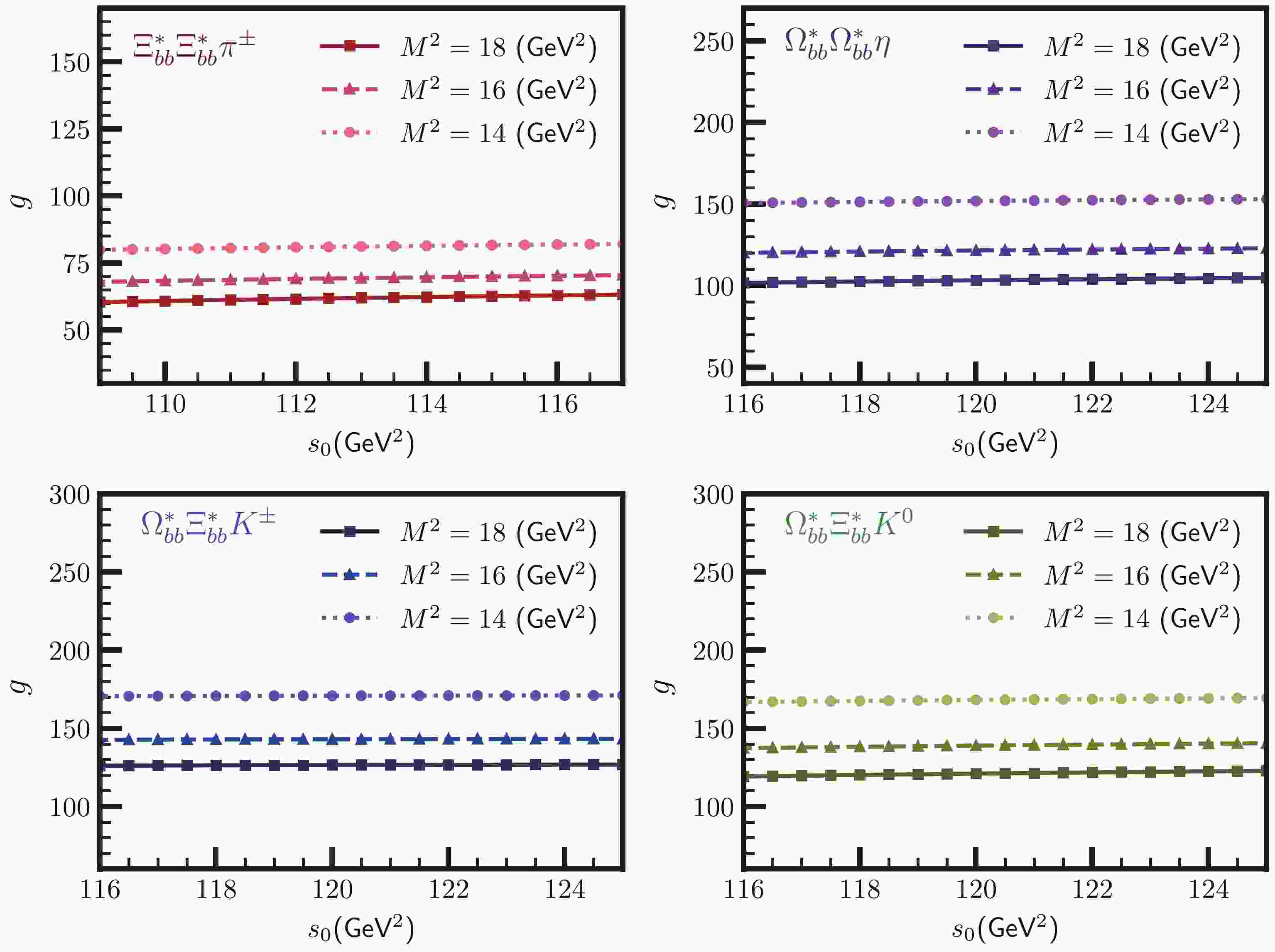
$ s_0 $ and Borel parameter$ M^2 $ . To this end, we imposed the conditions of OPE convergence, pole dominance, and relatively weak dependence of the results on auxiliary parameters. The threshold$ s_0 $ depends on the energy of the first excited state at each channel. We did not have any experimental information on the excited states of the doubly heavy baryons. However, our analyses show that in the interval$ m_{B^*}+ 0.3 \leqslant\sqrt{s_0}\leqslant $ $ m_{B^*}+ 0.5 \; \text{GeV} $ the standard requirements are satisfied. To fix the Borel parameter$ M^2 $ we proceeded with the following steps: for its upper limit, we imposed the condition of pole dominance; for its lower limit, we imposed the OPE convergence condition. These requirements led to the working regions 14$ \leqslant M^2 $ $ \leqslant 18 $ GeV2, 8$ \leqslant M^2 $ $ \leqslant 11 $ GeV2, and 4$ \leqslant M^2 $ $ \leqslant 6 $ GeV2 for the$ bb $ ,$ bc $ , and$ cc $ channels, respectively.In Fig. 1, as an example, we show the dependence of the coupling constant g on the continuum threshold at some fixed values of the Borel parameter for the vertices
$ \Xi^*_{bb}\Xi^*_{bb} \pi^{\pm} $ ,$ \Omega^*_{bb}\Omega^*_{bb} \eta $ ,$ \Omega^*_{bb}\Xi^*_{bb} K^{\pm} $ , and$ \Omega^*_{bb}\Xi^*_{bb} K^0 $ . Note that the strong coupling constants depend very weakly on$ s_0 $ . In another example, we show the dependence of g on the Borel parameter$ M^2 $ for the vertices$ \Xi^*_{bb}\Xi^*_{bb} \pi^{\pm} $ ,$ \Omega^*_{bb}\Omega^*_{bb} \eta $ ,$ \Omega^*_{bb}\Xi^*_{bb} K^{\pm} $ , and$ \Omega^*_{bb}\Xi^*_{bb} K^0 $ at fixed values of$ s_0 $ in Fig 2. From these plots, we see that the strong coupling constants show some dependence on the Borel parameter. This constitutes the main source of uncertainties. However, these uncertainties remain inside the limits allowed by the method.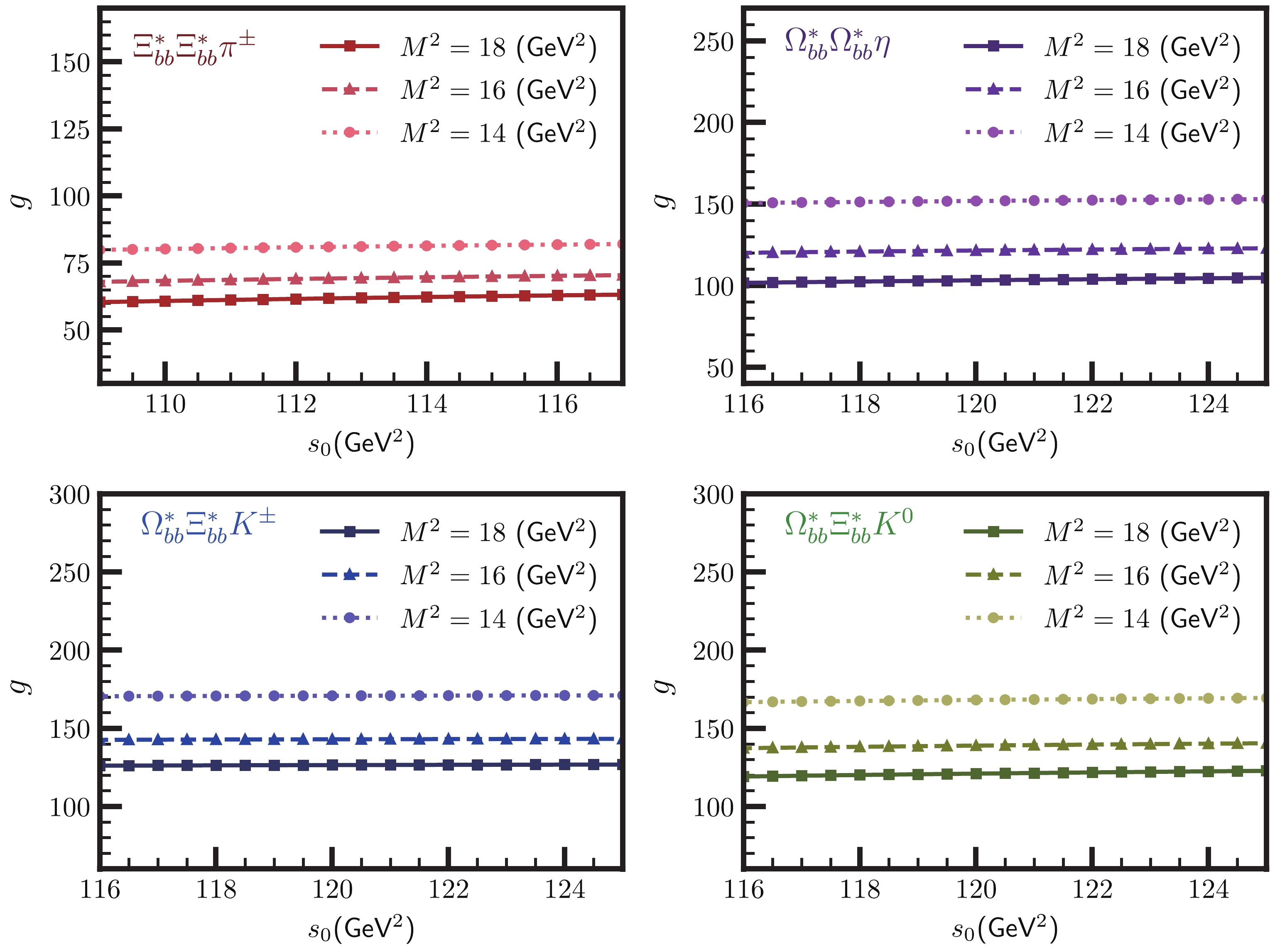
Figure 1. (color online) Dependence of the strong coupling constant g on the continuum threshold at different values of the Borel parameter
$ M^2 = $ 14, 16 and 18 GeV2.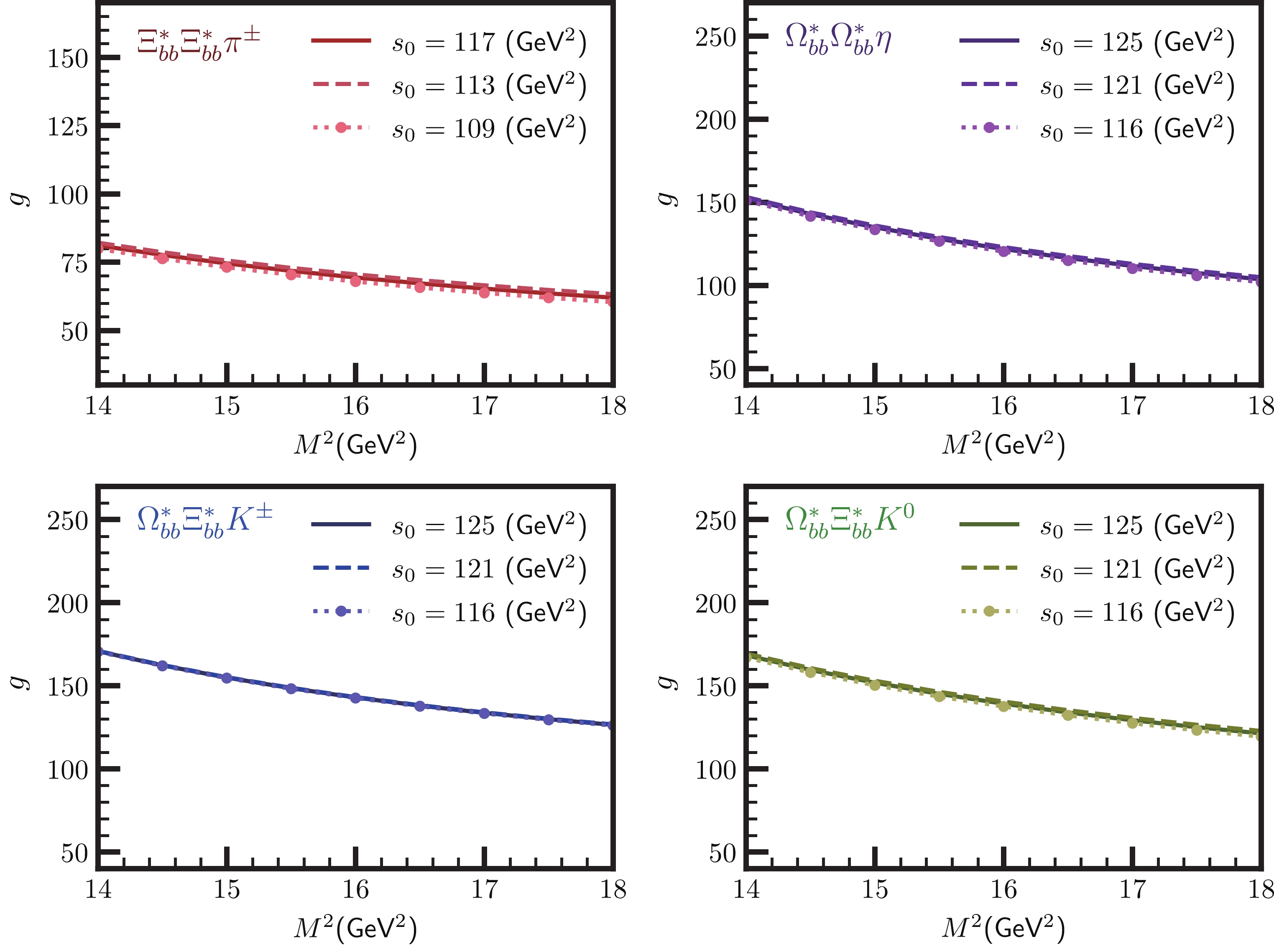
Figure 2. (color online) Dependence of the strong coupling constant g on the Borel parameter at different values of the continuum threshhold
$s_0$ . The lines correspond to$ s_0 = $ 109, 113, and 117 GeV2 for the$ \Xi^*_{bb}\Xi^*_{bb} \pi^{\pm} $ channel and$ s_0 = $ 116, 121, and 125 GeV2 for the$ \Omega^*_{bb}\Omega^*_{bb} \eta $ ,$ \Omega^*_{bb}\Xi^*_{bb} K^{\pm} $ , and$ \Omega^*_{bb}\Xi^*_{bb} K^0 $ channels.Taking into account all the input values as well as the working intervals for the auxiliary parameters, we extracted the numerical values for the strong coupling constants from the light-cone sum rules (46). The numerical results of g for all the considered vertices in
$ cc $ ,$ bc $ , and$ bb $ channels are presented in Table 5. There are three sources of errors in the results. The first is from the input parameters we used in the calculations. The second is the intrinsic error, which is due to the quark-hadron duality assumption. Finally, the third one is the error resulting from the variations with respect to the auxiliary parameters in their working intervals. The total error in the results amounts to 20%.Vertex $ M^2 $ /GeV2

$ s_0 $ /GeV2

strong coupling constant Decays to π $ \Xi^*_{bb} \Xi^*_{bb} \pi^0 $ 

$ 14\leqslant M^2\leqslant 18 $ 

$ 109\leqslant s_0\leqslant 117 $ 

$ 50.0^{\:7.9}_{\:7.8} $ 

$ \Xi^*_{bb} \Xi^*_{bb} \pi^\pm $ 

$ 14\leqslant M^2\leqslant 18 $ 

$ 109\leqslant s_0\leqslant 117 $ 

$ 70.8^{\:11.4}_{\:10.3} $ 

$ \Xi^*_{bc}\Xi^*_{bc} \pi^0 $ 

$ 7\leqslant M^2\leqslant 10 $ 

$ 57\leqslant s_0\leqslant 63 $ 

$ 13.4^{\:1.4}_{\:1.4} $ 

$ \Xi^*_{bc} \Xi^*_{bc} \pi^\pm $ 

$ 7\leqslant M^2\leqslant 10 $ 

$ 57\leqslant s_0\leqslant 63 $ 

$ 18.9^{\:2.0}_{\:2.0} $ 

$ \Xi^*_{cc} \Xi^*_{cc} \pi^0 $ 

$ 3\leqslant M^2\leqslant 6 $ 

$ 16\leqslant s_0\leqslant 19 $ 

$ 3.8^{\:0.3}_{\:0.4} $ 

$ \Xi^*_{cc} \Xi^*_{cc} \pi^\pm $ 

$ 3\leqslant M^2\leqslant 6 $ 

$ 16\leqslant s_0\leqslant 19 $ 

$ 5.5 ^{\:0.5}_{\:0.6} $ 

Decays to η $ \Omega^*_{bb} \Omega^*_{bb} \eta $ 

$ 14\leqslant M^2\leqslant 18 $ 

$ 116\leqslant s_0\leqslant 125 $ 

$ 125.7^{\:22.3}_{\:23.7} $ 

$ \Omega^*_{bc} \Omega^*_{bc} \eta $ 

$ 7\leqslant M^2\leqslant 10 $ 

$ 57\leqslant s_0\leqslant 64 $ 

$ 18.4^{\:2.1}_{\:2.0} $ 

$ \Omega^*_{cc} \Omega^*_{cc} \eta $ 

$ 3\leqslant M^2\leqslant 6 $ 

$ 16\leqslant s_0\leqslant 20 $ 

$ 5.9^{\:0.5}_{\:0.6} $ 

Decays to K $ \Omega^*_{bb} \Xi^*_{bb} K^0 $ 

$ 14\leqslant M^2\leqslant 18 $ 

$ 116\leqslant s_0\leqslant 125 $ 

$ 142.9^{\:26.6}_{\:23.4} $ 

$ \Omega^*_{bb} \Xi^*_{bb} K^\pm $ 

$ 14\leqslant M^2\leqslant 18 $ 

$ 116\leqslant s_0\leqslant 125 $ 

$ 142.3^{\:26.4}_{\:23.2} $ 

$ \Omega^*_{bc} \Xi^*_{bc} K^0 $ 

$ 7\leqslant M^2\leqslant 10 $ 

$ 57\leqslant s_0\leqslant 64 $ 

$ 27.5^{\:3.0}_{\:2.9} $ 

$ \Omega^*_{bc} \Xi^*_{bc} K^\pm $ 

$ 7\leqslant M^2\leqslant 10 $ 

$ 57\leqslant s_0\leqslant 64 $ 

$ 27.3^{\:3.0}_{\:2.9} $ 

$ \Omega^*_{cc} \Xi^*_{cc} K^0 $ 

$ 3\leqslant M^2\leqslant 6 $ 

$ 16\leqslant s_0\leqslant 20 $ 

$ 8.7^{\:0.8}_{\:0.9} $ 

$ \Omega^*_{cc} \Xi^*_{cc} K^\pm $ 

$ 3\leqslant M^2\leqslant 6 $ 

$ 16\leqslant s_0\leqslant 20 $ 

$ 8.6^{\:0.7}_{\:0.9} $ 

Table 5. Working regions of the Borel parameter
$ M^2 $ and continuum threshold$ s_0 $ as well as numerical values for different strong coupling constants extracted from the analyses. -
In the present study, we investigated the strong coupling constants of the doubly heavy spin-
$ 3/2 $ baryons,$ \Omega^*_{QQ'} $ and$ \Xi^*_{QQ'} $ , with the light pseudoscalar mesons, π, K, and η, by applying the LCSR formalism. We used the interpolating currents of the doubly heavy baryons and DAs of the mesons to construct the sum rules for the strong coupling constants. By fixing the auxiliary parameters, we addressed the calculations through the Borel transformation as well as continuum subtraction. We obtained the numerical results for different possible vertices considering the quark contents of the participating particles and other considerations.The results show that the heavier the doubly heavy baryons, the larger their strong couplings to the same pseudoscalar mesons. The significant difference between the c- and b-baryons can be explained using the heavy-quark spin symmetry, which states that the partial strong decay widths of heavy quark hadronic systems are independent of the heavy quark flavor and spin [74]. Considering the Fermi golden rule and the fact that the amplitude is proportional to the strong coupling constant, defining the corresponding vertex immediately implies that the heavier the doubly-heavy baryon, the larger the strong coupling constant. Moreover, comparing with the results presented in Ref. [47], the values of the strong coupling constants among the doubly heavy spin-3/2 baryons and light pseudoscalar mesons are mostly larger than that of the spin-1/2 baryons with the same mesons according to Ref. [47].
Our results may help experimental groups in analyses of data including the hadrons examined in the present study. The results may also be used in the construction of strong potentials among the doubly heavy baryons and pseudoscalar mesons.
Strong vertices of doubly heavy spin-3/2 baryons with light pseudoscalar mesons
- Received Date: 2021-06-21
- Available Online: 2021-11-15
Abstract: The strong coupling constants are basic quantities that carry information on the strong interactions among the baryon and meson multiplets as well as information on the nature and internal structures of the involved hadrons. These parameters are introduced in the transition matrix elements of various decays as main inputs and play key roles in analyses of experimental data including various hadrons. We derive the strong coupling constants among the doubly heavy spin-


 DownLoad: