


 Abstract
 HTML
HTML Reference
 Related
 PDF
PDF


-
Based on the quantum field theories with gauge symmetries, the Standard Model (SM) has proved to be extremely successful in the description of strong, electromagnetic, and weak interactions among elementary particles in nature. However, the fermion mass spectra, flavor mixing patterns, and CP violation have been completely unexplained in the SM [1]. In particular, the discovery of neutrino oscillations calls for new physics beyond the SM to accommodate tiny neutrino masses and significant leptonic flavor mixing. Apart from the direct searches for new physics at the high-energy frontiers, another important approach is to precisely measure the basic properties of the SM particles and look for clear deviations from the SM predictions.
Very recently, the Muon
$ (g-2) $ Collaboration at the Fermi National Laboratory in the US released the precise measurement of the anomalous muon magnetic moment$ a^{}_\mu \equiv (g^{}_\mu - 2)/2 $ and found a$ 4.2\sigma $ discrepancy with the SM prediction [2], when combined with the final result from the E821 experiment at the Brookhaven National Laboratory in 2006 [3]. The reported difference between the combined experimental result$ a^{\rm{exp}}_\mu = 116\ 592\ 061(41) \times $ $ 10^{-11} $ [2] and the SM prediction$ a^{\rm{SM}}_\mu = 116\ 591\ 810(43) \times $ $ 10^{-11} $ [4-42] of the anomalous muon magnetic moment is$ \Delta a^{}_\mu \equiv a^{\rm{exp}}_\mu - a^{\rm{SM}}_\mu = 251(59) \times 10^{-11} \; , $

(1) where the
$ 1\sigma $ error in the last two digits is given by the number in the parentheses. Although such a discrepancy must be further scrutinized by more experimental data and more reliable calculations [43], it has already stimulated a great number of theoretical works on the new physics interpretations and their connections to other fundamental problems in particle physics, astronomy, and cosmology [44-89]. See, e.g., Refs. [44, 54], for an excellent summary of new-physics scenarios and earlier references.Motivated by this exciting progress, we propose a simple but viable model to simultaneously account for neutrino masses, leptonic flavor mixing, and the anomalous muon magnetic moment. The basic idea is to augment the type-(I+II) seesaw model [90-96] by introducing the
$ {{U}}(1)^{}_{L^{}_\mu - L^{}_\tau} $ gauge symmetry [97-99] and an additional singlet scalar field S. The results obtained in the present work are distinct from those reported in previous works in at least two aspects. First, the flavor-dependent gauge symmetry$ {{U}}(1)^{}_{L^{}_\mu - L^{}_\tau} $ places very restrictive constraints on the lepton flavor structures, so it is nontrivial to correctly reproduce in a simple way two neutrino mass-squared differences and three flavor mixing angles, as observed in the neutrino oscillation experiments [100-110]. In our model, the singlet scalar field S and triplet Higgs ∆ are assigned with the opposite charges$ Q^{}_{\mu\tau}(S) = +1 $ and$ Q^{}_{\mu\tau}(\Delta) = - 1 $ under the$ {{U}}(1)^{}_{L^{}_\mu - L^{}_\tau} $ symmetry, respectively. As a consequence, the effective Majorana mass matrix$ M^{}_\nu $ of three light neutrinos can take the two-zero texture$ {\boldsymbol{B}}^{}_3 $ [111-113], which leads to readily testable predictions for the neutrino mixing parameters [114, 115]. Second, we point out that both the contributions from the Higgs triplet and those from the heavy Majorana neutrinos to$ \Delta a^{}_\mu $ appear with a negative sign. Therefore, the observed discrepancy$ \Delta a^{}_\mu $ can only be explained by the contribution from the gauge boson$ Z^\prime $ associated with the$ {{U}}(1)^{}_{L^{}_\mu - L^{}_\tau} $ gauge symmetry. As there is no tree-level interaction between the electrons and$ Z^\prime $ , the anomalous electron magnetic moment$ \Delta a^{}_e \equiv a^{\rm{exp}}_e - a^{\rm{SM}}_e $ receives the dominant correction from the Higgs triplet, implying a negative sign of$ \Delta a^{}_e $ that remains consistent with the experimental observation at the$ 2\sigma $ level. Our model offers an explicit example to realize the opposite signs for$ \Delta a^{}_\mu $ and$ \Delta a^{}_e $ in the same framework.The rest of this paper is organized as follows. In Sec. II, we introduce the extended version of the type-(I+II) model with a gauged
$ L^{}_\mu - L^{}_\tau $ symmetry, and explain its main features. The phenomenological implications for neutrino masses and flavor mixing are discussed in Sec. III, while the anomalous electron and muon magnetic moments are calculated in Sec. IV. Finally, some concluding remarks are presented in Sec. V. -
Although the individual lepton numbers
$ L^{}_\alpha $ (for$ \alpha = e, \mu, \tau $ ) and the baryon number B happen to be conserved in the SM at the classical level, they are actually violated by quantum anomalies [116]. However, the differences between any two of these global charges, such as$ B/3 - L^{}_\alpha $ (for$ \alpha = e, \mu, \tau $ ),$ L^{}_e - L^{}_\mu $ , and$ L^{}_\mu - L^{}_\tau $ , are anomaly-free and can naturally be promoted to gauge symmetries. The well-established phenomena of neutrino oscillations, in particular the approximate$ \mu $ -$ \tau $ exchange or reflection symmetries observed in the neutrino flavor mixing [117], indicate that the$ {{U}}(1)^{}_{L^{}_\mu - L^{}_\tau} $ gauge symmetry can be compatible with the experimental observations.In the canonical type-(I+II) seesaw model, where three right-handed neutrino singlets
$ \nu^{}_{\alpha {\rm{R}}} $ (for$ \alpha = e, \mu, \tau $ ) and one Higgs triplet ∆ under the$ {{SU}}(2)^{}_{\rm{L}} $ gauge symmetry are added into the SM particle content, it is natural to obtain tiny Majorana masses of three ordinary neutrinos. However, the flavor structures of the lepton Yukawa couplings and right-handed neutrino mass matrix are entirely unconstrained in the type-(I+II) seesaw model. As we shall see in the next section, the$ {{U}}(1)^{}_{L^{}_\mu - L^{}_\tau} $ gauge symmetry could impose tight constraints on the lepton flavor structures. Usually, the flavor structures are constrained to be too simple to accommodate two neutrino mass-squared differences$ \Delta m^2_{ij} \equiv m^2_i - m^2_j $ (for$ ij = 21, 31 $ ) and three neutrino mixing angles$ \{\theta^{}_{12}, \theta^{}_{13}, \theta^{}_{23}\} $ extracted from the neutrino oscillation experiments. For this reason, we have to modify the canonical type-(I+II) seesaw model in the most economical way by introducing an additional complex scalar S, which is singlet under the SM gauge symmetry but possesses a nontrivial$ {{U}}(1)^{}_{L^{}_\mu - L^{}_\tau} $ charge. The relevant fields and their charges under the overall gauge symmetry$ {{SU}}(2)^{}_{\rm{L}}\otimes {{U}}(1)^{}_{\rm{Y}}\otimes {{U}}(1)^{}_{L^{}_\mu - L^{}_\tau} $ have been summarized in Table 1. In what follows, we explain the extra terms appearing in the gauge-invariant Lagrangian and briefly discuss their phenomenological implications.$ \ell^{}_{e{\rm{L}}}, \ell^{}_{\mu{\rm{L}}}, \ell^{}_{\tau{\rm{L}}} $ 

$ e^{}_{\rm{R}}, \mu^{}_{\rm{R}}, \tau^{}_{\rm{R}} $ 

$ \nu^{}_{e{\rm{R}}}, \nu^{}_{\mu{\rm{R}}}, \nu^{}_{\tau{\rm{R}}} $ 

S H ∆ ${{SU} }(2)^{}_{\rm{L} }\otimes U(1)^{}_{\rm{Y} }$ 

(2, −1) (1, −2) (1, 0) (1, 0) (2, +1) (3, −2) $ U(1)^{}_{L^{}_\mu - L^{}_\tau}$ 

0, +1, −1 0, +1, −1 0, +1, −1 +1 0 −1 Table 1. Charge assignments of the relevant fields under the
$ {{SU}}(2)^{}_{\rm{L}}\otimes {{U}}(1)^{}_{\rm{Y}}\otimes {{U}}(1)^{}_{L^{}_\mu - L^{}_\tau} $ gauge symmetry in the extended type-(I+II) seesaw model.First, there is a new gauge symmetry, for which the gauge field is denoted as
$ Z^\prime_\mu $ and the gauge boson as$ Z^\prime $ . In addition to the new kinetic term① composed of the field-strength tensor$ Z^\prime_{\mu\nu} \equiv \partial^{}_\mu Z^\prime_\nu - \partial^{}_\nu Z^\prime_\mu $ , the covariant derivative will be modified to$ D^\prime_\mu \equiv \partial^{}_\mu - {\rm i} g \tau^a W^a_\mu - {\rm i} g^\prime \frac{Y}{2} B^{}_\mu - {\rm i} g^{}_{Z^\prime} Q^{}_{\mu\tau} Z^\prime_\mu \; , $

(2) where
$ Q^{}_{\mu\tau} $ represents the charge under the$ {{U}}(1)^{}_{L^{}_\mu - L^{}_\tau} $ symmetry (cf. the charges in the last row of Table 1), and$ g^{}_{Z^\prime} $ is the corresponding gauge coupling. As only the SM leptons and right-handed neutrinos of the muon and tauon flavors are charged fermions under such a gauge symmetry, the neutral-current interactions of these fermions with$ Z^\prime_\mu $ read$\begin{aligned}[b] {\cal{L}}^\prime_{\rm{NC}} =& g^{}_{Z^\prime} \Big[\left(\overline{\ell^{}_{\mu {\rm{L}}}} \gamma^\mu \ell^{}_{\mu {\rm{L}}} - \overline{\ell^{}_{\tau {\rm{L}}}} \gamma^\mu \ell^{}_{\tau {\rm{L}}}\right) + \left( \overline{\mu^{}_{\rm{R}}} \gamma^\mu \mu^{}_{\rm{R}} - \overline{\tau^{}_{\rm{R}}} \gamma^\mu \tau^{}_{\rm{R}} \right) \\& +\left( \overline{\nu^{}_{\mu{\rm{R}}}} \gamma^\mu \nu^{}_{{\mu}{\rm{R}}} - \overline{\nu^{}_{{\tau}{\rm{R}}}} \gamma^\mu \nu^{}_{{\tau}{\rm{R}}} \right)\Big]Z^\prime_\mu \; , \end{aligned} $

(3) where the interaction terms in the first two round brackets on the right-hand side contribute to the muon
$ (g-2) $ , as we shall see later.Second, the scalar potential of the model considerably resembles that of the type-II seesaw model [118], where only one Higgs triplet is introduced into the SM. With an extra singlet scalar S, we can immediately determine the gauge-invariant scalar potential as
$ \begin{aligned}[b] V(S, H, \Delta) = & -\mu^2_H H^\dagger H + \lambda^{}_H (H^\dagger H)^2 - \mu^2_S S^\dagger S + \lambda^{}_S (S^\dagger S)^2 \\&+ \frac{1}{2} M^2_\Delta {\rm{Tr}}(\Delta^\dagger \Delta) + \left(\lambda^{}_{1} S H^{\rm{T}} {\rm{i}}\sigma^{}_2 \Delta H + {\rm{h.c.}} \right)\\& + \frac{\lambda^{}_2}{2} (H^\dagger H) {\rm{Tr}}(\Delta^\dagger \Delta) + \frac{\lambda^{}_3}{4} (H^\dagger \sigma^{}_i H) {\rm{Tr}}(\Delta^\dagger \sigma^{}_i \Delta) \\&+ \frac{\lambda^{}_4}{2} (S^\dagger S) {\rm{Tr}}(\Delta^\dagger \Delta) + \frac{\lambda^{}_5}{2} (S^\dagger S) (H^\dagger H) \\&+ \frac{\lambda^{}_6}{4} {\rm{Tr}}\left[ (\Delta^\dagger \Delta)^2\right] + \frac{\lambda^{}_7}{4} \left[{\rm{Tr}}(\Delta^\dagger \Delta)\right]^2 \; , \end{aligned}$

(4) where the coupling constant
$ \lambda^{}_1 $ is, in general, complex. It should be noted that the coefficient of the trilinear coupling term of the SM Higgs doublet H and the Higgs triplet ∆ is of mass dimension and small in the type-II seesaw model, whereas it is now given by$ \lambda^{}_1 \langle S \rangle = \lambda^{}_1 v^{}_S $ after the singlet scalar acquires its vacuum expectation value (vev). Instead of a complete analysis of the vacuum structure based on the scalar potential$ V(S, H, \Delta) $ , we make some reasonable approximations and recapitulate the main features of the spontaneous symmetry breaking in our model.● The general scalar potential in Eq. (4) can be greatly simplified if some quartic couplings (e.g.,
$ \lambda^{}_3 $ ,$ \lambda^{}_4 $ ,$ \lambda^{}_5 $ , and$ \lambda^{}_7 $ ) are set to zero. In this case, the physical triplet scalars$ H^{\pm \pm} $ ,$ H^\pm $ ,$ H^0 $ , and$ A^0 $ are degenerate in mass, namely,$ M^{}_{H^{\pm\pm}} = M^{}_{H^\pm} = M^{}_{H^0} = M^{}_{A^0} = M^{}_\Delta $ . Meanwhile, the vev's of the neutral scalar bosons are approximately given by$ v^{}_S \approx \sqrt{\mu^2_S/\lambda^{}_S} $ ,$ v^{}_H \approx \sqrt{\mu^2_H/\lambda^{}_H} $ , and$ v^{}_\Delta \approx \lambda^{}_1 v^{}_S v^2_H/M^2_\Delta $ . It should be noted that the coupling constant$ \lambda^{}_1 $ can be made real by redefining the phases of the scalar fields S, H, and ∆.● The singlet scalar field S is only charged under the
$ {{U}}(1)^{}_{L^{}_\mu - L^{}_\tau} $ gauge symmetry, so the mass of the gauge boson$ Z^\prime $ is given by$ M^{}_{Z^\prime} = g^{}_{Z^\prime} v^{}_S/2 $ . As the Higgs triplet carries the charges of all three gauge symmetries, it induces mass mixing among the three neutral gauge bosons Z,$ Z^\prime $ , and$ \gamma $ after the spontaneous symmetry breaking. However, as the vev of the triplet Higgs is constrained severely by the precision measurement of the$ \rho $ parameter [119], namely,$ \rho \equiv M^2_W/(M^2_Z \cos^2 \theta^{}_{\rm{W}}) \approx (v^2_H + 2v^2_\Delta)/(v^2_H + $ $ 4 v^2_\Delta) = 1.00038 \pm 0.00020 $ , from which one can set an upper bound$ v^{}_\Delta \lesssim 2.58\; {\rm{GeV}} $ at the$ 3\sigma $ level for$ v^{}_H \approx $ $ 246\; {\rm{GeV}} $ , one expects that$ M^{}_{Z^\prime} $ is mainly determined by the gauge coupling$ g^{}_{Z^\prime} $ and the vev$ v^{}_S $ of the singlet scalar. In our case,$ v^{}_\Delta $ also contributes to the light neutrino masses, and thus, its magnitude is further required to be below$ 1\; {\rm{eV}} $ . Consequently, the dominant decay channel of the doubly-charged and singly-charged Higgs bosons is purely leptonic.Third, the gauge-invariant Yukawa interactions and mass terms for the leptons are given by
$ \begin{aligned}[b] {\cal{L}}^{}_{\rm{lepton}} =& - y^\alpha_l \overline{\ell^{}_{\alpha {\rm{L}}}} \alpha^{}_{\rm{R}} H - \frac{1}{2} y^{}_\Delta \left( \overline{\ell^{}_{e{\rm{L}}}} \Delta {\rm{i}}\sigma^{}_2 \ell^{\rm{C}}_{\tau {\rm{L}}} + \overline{\ell^{}_{\tau{\rm{L}}}} \Delta {\rm{i}}\sigma^{}_2 \ell^{\rm{C}}_{e {\rm{L}}}\right)\\& - y^\alpha_\nu \overline{\ell^{}_{\alpha {\rm{L}}}} \tilde{H} \nu^{}_{\alpha {\rm{R}}} - \frac{1}{2} y^{e\tau}_{S} \left( \overline{\nu^{\rm{C}}_{e{\rm{R}}}} \nu^{}_{\tau {\rm{R}}} + \overline{\nu^{\rm{C}}_{\tau{\rm{R}}}} \nu^{}_{e {\rm{R}}} \right) S\\& - \frac{1}{2} y^{e\mu}_{S} \left( \overline{\nu^{\rm{C}}_{e{\rm{R}}}} \nu^{}_{\mu {\rm{R}}} + \overline{\nu^{\rm{C}}_{\mu{\rm{R}}}} \nu^{}_{e {\rm{R}}} \right) S^\dagger \\& - \frac{1}{2} \left[ m^{ee}_{\rm{R}} \overline{\nu^{\rm{C}}_{e {\rm{R}}}} \nu^{}_{e {\rm{R}}} + m^{\mu\tau}_{\rm{R}} \left(\overline{\nu^{\rm{C}}_{\mu {\rm{R}}}} \nu^{}_{\tau {\rm{R}}} + \overline{\nu^{\rm{C}}_{\tau {\rm{R}}}} \nu^{}_{\mu {\rm{R}}} \right)\right] + {\rm{h.c.}} \; , \end{aligned}$

(5) which, after the spontaneous symmetry breaking with
$ \langle H \rangle = v^{}_H/\sqrt{2} $ ,$ \langle \Delta \rangle = v^{}_\Delta $ , and$ \langle S \rangle = v^{}_S/\sqrt{2} $ , leads to the lepton mass matrices$ \begin{aligned}[b]& M_l^{} = \frac{{v_H^{}}}{{\sqrt 2 }}\left( {\begin{array}{*{20}{c}} {y_l^e}&0&0\\ 0&{y_l^\mu }&0\\ 0&0&{y_l^\tau } \end{array}} \right)\;,\\& M_{\rm{D}}^{} = \frac{{v_H^{}}}{{\sqrt 2 }}\left( {\begin{array}{*{20}{c}} {y_\nu ^e}&0&0\\ 0&{y_\nu ^\mu }&0\\ 0&0&{y_\nu ^\tau } \end{array}} \right)\;,\end{aligned} $

(6) and
$ \begin{aligned}[b] &M_{\rm{L}}^{} = \left( {\begin{array}{*{20}{c}} 0&0&{y_\Delta ^{}v_\Delta ^{}}\\ 0&0&0\\ {y_\Delta ^{}v_\Delta ^{}}&0&0 \end{array}} \right)\;,\\& M_{\rm{R}}^{} = \left( {\begin{array}{*{20}{c}} {m_{\rm{R}}^{ee}}&{y_S^{e\mu }v_S^{}/\sqrt 2 }&{y_S^{e\tau }v_S^{}/\sqrt 2 }\\ {y_S^{e\mu }v_S^{}/\sqrt 2 }&0&{m_{\rm{R}}^{\mu \tau }}\\ {y_S^{e\tau }v_S^{}/\sqrt 2 }&{m_{\rm{R}}^{\mu \tau }}&0 \end{array}} \right)\;.\end{aligned} $

(7) Before discussing the details of the neutrino masses and leptonic flavor mixing, we examine the relevant model parameters in the leptonic sector. First, as indicated in Eq. (5), the charged-lepton Yukawa coupling matrix
$ Y^{}_l \equiv {\rm{Diag}}\{y^e_l, y^\mu_l, y^\tau_l \} $ is diagonal, and one can always choose the coupling constants$ y^\alpha_l $ (for$ \alpha = e, \mu, \tau $ ) to be real by redefining the phases of the right-handed charged-lepton fields. In this case, the charged-lepton masses are simply given by$ m^{}_\alpha = y^\alpha_l v^{}_H/\sqrt{2} $ (for$ \alpha = e, \mu, \tau $ ). Second, without loss of generality, we can also make the Dirac neutrino Yukawa coupling constants$ y^\alpha_\nu $ (for$ \alpha = e, \mu, \tau $ ) all real by absorbing their phases into the left-handed lepton doublets. In addition, the overall phase of$ y^{}_\Delta $ can be removed by rephasing the Higgs triplet ∆, so the type-II Majorana neutrino mass matrix$ M^{}_{\rm{L}} $ is symmetric and real. Finally, one can eliminate the phases of the mass parameters$ m^{ee}_{\rm{R}} $ and$ m^{\mu\tau}_{\rm{R}} $ by utilizing the freedom of redefining the phases of the right-handed neutrinos. However, it is impossible to choose both$ y^{e\mu}_S $ and$ y^{e\tau}_S $ to be real, even with the phase redefinition of the singlet scalar field S. For illustration, we consider$ y^{e\mu}_S $ to be complex and all the other model parameters to be real and positive in the following discussions. The other case with a complex$ y^{e\tau}_S $ but real$ y^{e\mu}_S $ can be similarly studied. -
As the Dirac neutrino mass matrix
$ M^{}_{\rm{D}} = {\rm{Diag}} \{d^{}_e, $ $ d^{}_\mu, d^{}_\tau\} $ with$ d^{}_\alpha \equiv y^\alpha_\nu v^{}_H/\sqrt{2} $ is simply diagonal, the leptonic flavor mixing arises solely from the flavor structure of$ M^{}_{\rm{R}} $ and its interplay with the contribution from the Higgs triplet. Without the Higgs triplet, the phenomenological implications for the neutrino masses and leptonic flavor mixing have been thoroughly studied in a numerical way in the literature [105]. In the assumption of$ y^{e\tau}_S \ll |y^{e\mu}_S| $ , we found that it is possible to perform an analytical calculation, which can manifest the direct correlation between the model parameters and physical observables.Ignoring the element
$ y^{e\tau}_S v^{}_S/\sqrt{2} $ in the Majorana mass matrix of the right-handed neutrinos$ M^{}_{\rm{R}} $ , we observe that it can be exactly diagonalized via the orthogonal transformation$ U^\dagger M^{}_{\rm{R}} U^* = \widehat{M}^{}_{\rm{R}} = {\rm{Diag}}\{M^{}_1, M^{}_2, M^{}_3\} $ , where$ M^{}_i $ (for$ i = 1, 2, 3 $ ) are heavy Majorana neutrino masses and related to the real and positive parameters by [120, 121]$ m^e_{\rm{R}} = M^{}_3 (1 - y^{}_{\rm{R}} + x^{}_{\rm{R}} y^{}_{\rm{R}}) \; , $

(8) $ \frac{|y^{e\mu}_S| v^{}_S}{\sqrt{2}} = M^{}_3 \left[ \frac{y^{}_{\rm{R}} (1 - x^{}_{\rm{R}}) (1 - y^{}_{\rm{R}}) (1 + x^{}_{\rm{R}} y^{}_{\rm{R}})}{1 - y^{}_{\rm{R}} + x^{}_{\rm{R}} y^{}_{\rm{R}}} \right]^{1/2} \; , $

(9) $ m^{\mu\tau}_{\rm{R}} = M^{}_3 \left( \frac{x^{}_{\rm{R}} y^2_{\rm{R}}}{1 - y^{}_{\rm{R}} + x^{}_{\rm{R}} y^{}_{\rm{R}}} \right)^{1/2} \; , $

(10) where the mass ratios
$ x^{}_{\rm{R}} \equiv M^{}_1/M^{}_2 $ and$ y^{}_{\rm{R}} \equiv M^{}_2/M^{}_3 $ have been defined with both$ x^{}_{\rm{R}} $ and$ y^{}_{\rm{R}} $ being in the range$ (0, 1) $ . The nine elements$ U^{}_{\alpha i} $ (for$ \alpha = e, \mu, \tau $ and$ i = 1, 2, 3 $ ) of the unitary matrix U are explicitly given by [121]$ \begin{aligned}[b] U^{}_{e1} =& - \left[ \frac{x^{}_{\rm{R}}y^{}_{\rm{R}}(1-x^{}_{\rm{R}})(1+x^{}_{\rm{R}}y^{}_{\rm{R}})}{(1+x^{}_{\rm{R}})(1-x^{}_{\rm{R}}y^{}_{\rm{R}})(1-y^{}_{\rm{R}}+x^{}_{\rm{R}}y^{}_{\rm{R}})} \right]^{1/2} \; , \\ U^{}_{e2} =& -{\rm{i}} \left[ \frac{y^{}_{\rm{R}} (1 - x^{}_{\rm{R}}) (1 - y^{}_{\rm{R}})}{(1 + x^{}_{\rm{R}}) (1 + y^{}_{\rm{R}}) (1 - y^{}_{\rm{R}} + x^{}_{\rm{R}} y^{}_{\rm{R}})} \right]^{1/2} \; , \\ U^{}_{e3} =& + \left[ \frac{(1 - y^{}_{\rm{R}}) (1 + x^{}_{\rm{R}} y^{}_{\rm{R}})}{(1 - x^{}_{\rm{R}} y^{}_{\rm{R}})(1 + y^{}_{\rm{R}})(1 - y^{}_{\rm{R}} + x^{}_{\rm{R}} y^{}_{\rm{R}})} \right]^{1/2} \; , \\ U^{}_{\mu 1} =& + {\rm e}^{{\rm{i}}\phi} \left[ \frac{x^{}_{\rm{R}}(1 - y^{}_{\rm{R}})}{(1 + x^{}_{\rm{R}}) (1 - x^{}_{\rm{R}} y^{}_{\rm{R}})} \right]^{1/2} \; , \\ U^{}_{\mu 2} =& + {\rm{i}} {\rm e}^{{\rm{i}}\phi} \left[ \frac{1 + x^{}_{\rm{R}} y^{}_{\rm{R}}}{(1 + x^{}_{\rm{R}}) (1 + y^{}_{\rm{R}})} \right]^{1/2} \; , \\ U^{}_{\mu 3} =& + {\rm e}^{{\rm{i}}\phi} \left[ \frac{y^{}_{\rm{R}} (1 - x^{}_{\rm{R}})}{(1 - x^{}_{\rm{R}} y^{}_{\rm{R}})(1 + y^{}_{\rm{R}})} \right]^{1/2} \; , \\ U^{}_{\tau 1} = & + {\rm e}^{-{\rm{i}}\phi} \left[ \frac{1 - y^{}_{\rm{R}}}{(1 + x^{}_{\rm{R}})(1 - x^{}_{\rm{R}} y^{}_{\rm{R}})(1 - y^{}_{\rm{R}} + x^{}_{\rm{R}} y^{}_{\rm{R}})} \right]^{1/2} \; , \\ U^{}_{\tau 2} =& -{\rm{i}} {\rm e}^{-{\rm{i}}\phi} \left[ \frac{x^{}_{\rm{R}}(1 + x^{}_{\rm{R}} y^{}_{\rm{R}})}{(1 + x^{}_{\rm{R}})(1 + y^{}_{\rm{R}})(1 - y^{}_{\rm{R}} + x^{}_{\rm{R}} y^{}_{\rm{R}})} \right]^{1/2} \; , \\ U^{}_{\tau 3} =& + {\rm e}^{-{\rm{i}}\phi} \left[ \frac{x^{}_{\rm{R}}y^3_{\rm{R}}(1 - x^{}_{\rm{R}})}{(1 - x^{}_{\rm{R}} y^{}_{\rm{R}}) (1 + y^{}_{\rm{R}}) (1 - y^{}_{\rm{R}} + x^{}_{\rm{R}} y^{}_{\rm{R}})} \right]^{1/2} \; , \end{aligned}$

(11) where the phase
$ \phi $ is defined as$ y^{e\mu}_S \equiv |y^{e\mu}_S| {\rm e}^{{\rm{i}}\phi} $ . From the above discussions, three heavy Majorana neutrino masses$ M^{}_i $ (for$ i = 1, 2, 3 $ ) or equivalently$ \{x^{}_{\rm{R}}, y^{}_{\rm{R}}, M^{}_3\} $ can be implemented to replace the model parameters$ m^e_{\rm{R}} $ ,$ |y^{e\mu}_S| v^{}_S $ , and$ m^{\mu\tau}_{\rm{R}} $ . The effective Majorana mass matrix of the three light neutrinos can be obtained from the type-(I+II) seesaw formula, i.e.,$ M^{}_\nu \approx M^{}_{\rm{L}} - M^{}_{\rm{D}} M^{-1}_{\rm{R}} M^{\rm{T}}_{\rm{D}} \; , $

(12) from which the explicit expressions of the six independent matrix elements are found to be
$ \begin{aligned}[b] \left(M^{}_\nu\right)^{}_{ee} =& - \frac{d^2_e}{M^{}_3} \cdot \frac{1}{1 - y^{}_{\rm{R}} + x^{}_{\rm{R}} y^{}_{\rm{R}}} \; , \\ \left(M^{}_\nu\right)^{}_{\mu\mu} = & 0 \; , \\ \left(M^{}_\nu\right)^{}_{\tau\tau} =& -\frac{d^2_\tau}{M^{}_3} \cdot \frac{(1 - x^{}_{\rm{R}}) (1 - y^{}_{\rm{R}}) (1 + x^{}_{\rm{R}} y^{}_{\rm{R}})}{x^{}_{\rm{R}} y^{}_{\rm{R}} (1 - y^{}_{\rm{R}} + x^{}_{\rm{R}} y^{}_{\rm{R}} )} \cdot {\rm e}^{2{\rm{i}} \phi} \; , \end{aligned} $

(13) and
$ \begin{aligned}[b] \left(M^{}_\nu\right)^{}_{e\mu} =& 0 \; , \\ \left(M^{}_\nu\right)^{}_{e\tau} =& y^{}_\Delta v^{}_\Delta + \frac{d^{}_e d^{}_\tau}{M^{}_3} \cdot \frac{1}{1 - y^{}_{\rm{R}} + x^{}_{\rm{R}} y^{}_{\rm{R}}} \\&\times \left[ \frac{(1 - x^{}_{\rm{R}}) (1 - y^{}_{\rm{R}}) (1 + x^{}_{\rm{R}} y^{}_{\rm{R}})}{x^{}_{\rm{R}} y^{}_{\rm{R}}} \right]^{1/2} \cdot {\rm e}^{{\rm{i}}\phi}\; , \\ \left(M^{}_\nu\right)^{}_{\mu\tau} =& -\frac{d^{}_\mu d^{}_\tau}{M^{}_3} \cdot \left( \frac{x^{}_{\rm{R}} y^2_{\rm{R}}}{1 - y^{}_{\rm{R}} + x^{}_{\rm{R}} y^{}_{\rm{R}}} \right)^{1/2} \; . \end{aligned} $

(14) One can immediately realize that the effective Majorana neutrino mass matrix
$ M^{}_\nu $ with$ (M^{}_\nu)^{}_{e\mu} = (M^{}_\nu)^{}_{\mu\mu} = 0 $ takes the form of the two-zero texture$ {\boldsymbol{B}}^{}_3 $ , for which the implications for the neutrino masses and leptonic flavor mixing have been carefully examined in the literature [114, 115]. Some helpful comments are as follows.● In the hierarchical limit of the heavy Majorana neutrino masses, i.e.,
$ M^{}_1 \ll M^{}_2 \ll M^{}_3 $ or equivalently$ x^{}_{\rm{R}}, y^{}_{\rm{R}} \ll 1 $ , the expressions of the nonzero neutrino mass matrix elements can be greatly simplified. More explicitly, we have$ \begin{aligned}[b]& \left(M^{}_\nu\right)^{}_{ee} = - d^2_e/M^{}_3 \\& \left(M^{}_\nu\right)^{}_{\tau\tau} = - d^2_\tau {\rm e}^{2{\rm{i}}\phi}/(M^{}_3 x^{}_{\rm{R}} y^{}_{\rm{R}})\\&\left(M^{}_\nu\right)^{}_{e\tau} = y^{}_\Delta v^{}_\Delta + d^{}_e d^{}_\tau {\rm e}^{{\rm{i}}\phi}/(M^{}_3 \sqrt{x^{}_{\rm{R}} y^{}_{\rm{R}}})\\& \left(M^{}_\nu\right)^{}_{\mu\tau} = - d^{}_\mu d^{}_\tau \times \rhbr \sqrt{x^{}_{\rm{R}}} y^{}_{\rm{R}}/M^{}_3\end{aligned}$

Because the charged-lepton mass matrix
$ M^{}_l = {\rm{Diag}}\{m^{}_e, m^{}_\mu, m^{}_\tau\} $ is diagonal, the effective neutrino mass matrix$ M^{}_\nu $ can be directly reconstructed from the leptonic mixing matrix V and three neutrino masses$ \widehat{M}^{}_\nu \equiv {\rm{Diag}}\{m^{}_1, m^{}_2, m^{}_3\} $ via$ M^{}_\nu = V \widehat{M}^{}_\nu V^{\rm{T}} $ . With precision measurements of the neutrino masses and flavor mixing parameters, one can extract very useful information about the model parameters from Eqs. (13) and (14).● For the two-zero texture
$ {\boldsymbol{B}}^{}_3 $ of the neutrino mass matrix$ M^{}_\nu $ , the zero elements results in serious constraints on the neutrino masses and flavor mixing parameters. Given$ (M^{}_\nu)^{}_{e\mu} = (M^{}_\nu)^{}_{\mu\mu} = 0 $ , we find [112-115]$ \begin{aligned}[b] \frac{\lambda^{}_1}{\lambda^{}_2} =& - \tan \theta^{}_{23} \cdot \frac{\sin \theta^{}_{12} \sin \theta^{}_{23} + \cos \theta^{}_{12} \cos \theta^{}_{23} \sin \theta^{}_{13} {\rm e}^{-{\rm{i}}\delta}}{\sin \theta^{}_{12} \cos \theta^{}_{23} - \cos \theta^{}_{12} \sin \theta^{}_{23} \sin \theta^{}_{13} {\rm e}^{+{\rm{i}}\delta}} \; , \\ \frac{\lambda^{}_2}{\lambda^{}_3} =& - \tan \theta^{}_{23} \cdot \frac{\cos \theta^{}_{12} \sin \theta^{}_{23} - \sin \theta^{}_{12} \cos \theta^{}_{23} \sin \theta^{}_{13} {\rm e}^{-{\rm{i}}\delta}}{\cos \theta^{}_{12} \cos \theta^{}_{23} + \sin \theta^{}_{12} \sin \theta^{}_{23} \sin \theta^{}_{13} {\rm e}^{+{\rm{i}}\delta}} \; , \end{aligned} $

(15) where
$ \lambda^{}_1 \equiv m^{}_1 {\rm e}^{2{\rm{i}}\rho} $ ,$ \lambda^{}_2 \equiv m^{}_2 {\rm e}^{2{\rm{i}}\sigma} $ , and$ \lambda^{}_3 \equiv m^{}_3 $ , with$ \rho $ and$ \sigma $ being two Majorana-type CP-violating phases. It can be observed that the standard parametrization of the leptonic flavor mixing matrix V has been adopted [119], where$ \{\theta^{}_{12}, \theta^{}_{13}, \theta^{}_{23}\} $ are three flavor mixing angles and$ \delta $ is the Dirac-type CP-violating phase. In the leading-order approximation, we ignore the terms proportional to$ \sin\theta^{}_{13} \approx 0.15 $ in Eq. (15) and thus observe that$ m^{}_1/m^{}_2 \approx m^{}_2/m^{}_3 \approx \tan^2 \theta^{}_{23} $ . Therefore, if the neutrino mass ordering is normal (i.e.,$ m^{}_1 < m^{}_2 < m^{}_3 $ ), then$ \theta^{}_{23} < 45^\circ $ should hold. Although the best-fit value$ \theta^{}_{23} \approx 49^\circ $ is found by the global-fit analysis of the current neutrino oscillation data [122], the values$ 39.6^\circ \lesssim \theta^{}_{23} \lesssim 51.8^\circ $ are still allowed at the$ 3\sigma $ level. If the neutrino mass ordering is inverted (i.e.,$ m^{}_3 < m^{}_1 < m^{}_2 $ ), then$ \theta^{}_{23} > 45^\circ $ is required. Such a correlation between the neutrino mass ordering and the octant of$ \theta^{}_{23} $ will definitely be tested in future neutrino oscillation experiments. At the next-to-leading order, one can determine the Dirac CP-violating phase via$ \cos \delta \approx - \frac{\Delta m^2_{21}}{\Delta m^2_{31}} \cdot \frac{\sin2\theta^{}_{12} \cot^2 \theta^{}_{23}}{2\sin \theta^{}_{13} \tan 2\theta^{}_{23}} \; , $

(16) where
$ \Delta m^2_{ij} \equiv m^2_i - m^2_j $ (for$ ij = 21, 31 $ ) are two neutrino mass-squared differences. In the case of normal neutrino mass ordering (i.e.,$ \Delta m^2_{21} > 0 $ and$ \Delta m^2_{31} > 0 $ ), we have$ \cos\delta < 0 $ because of$ \tan 2\theta^{}_{23} > 0 $ for$ \theta^{}_{23} < 45^\circ $ . It is straightforward to ascertain that$ \cos\delta < 0 $ is also valid in the case of inverted neutrino mass ordering.In summary, in the limit of
$ y^{e\tau}_S \ll |y^{e\mu}_S| $ , one can exactly diagonalize the right-handed neutrino mass matrix$ M^{}_{\rm{R}} $ , and the effective Majorana neutrino mass matrix$ M^{}_\nu \approx M^{}_{\rm{L}} - M^{}_{\rm{D}} M^{-1}_{\rm{R}} M^{\rm{T}}_{\rm{D}} $ emerges to be of the form of the two-zero texture$ {\boldsymbol{B}}^{}_3 $ . At the$ 3\sigma $ level, the predictions for the neutrino masses and flavor mixing parameters are compatible with the current neutrino oscillation data. As there exists a direct connection between the neutrino mass ordering and the octant of$ \theta^{}_{23} $ , the predictions will be well testable in the next-generation neutrino oscillation experiments. -
Apart from the neutrino oscillation parameters, the contributions from the new particles beyond the SM to the anomalous electron and muon magnetic moments can be calculated. To this end, it is helpful to specify the new particles appearing in the type-(I+II) seesaw model under consideration and their interactions with the charged leptons.
In addition to the electromagnetic interactions, there are three types of contributions to the charged-lepton magnetic moment in the SM [123-126], for which the Feynman diagrams are listed in Fig. 1. Because the electroweak contributions are well known, we focus only on the new-physics ones. Owing to the
$ {{U}}(1)^{}_{L^{}_\mu - L^{}_\tau} $ symmetry, the Higgs triplet ∆ is coupled only to the electron and tauon flavors in a flavor-changing way. As a consequence, it contributes to the anomalous magnetic moments of the electron and tauon, which will be considered later on. For the flavor-universal contributions, only the Feynman diagram shown in Fig. 1(b) involving massive Majorana neutrinos matters. This is actually the case in the type-I seesaw model. In the basis of the left-handed neutrino states$ \nu^{}_{\alpha {\rm{L}}} $ and$ \nu^{\rm{C}}_{\alpha {\rm{R}}} $ , the overall$ 6\times 6 $ mass matrix of the neutrinos can be diagonalized via [1]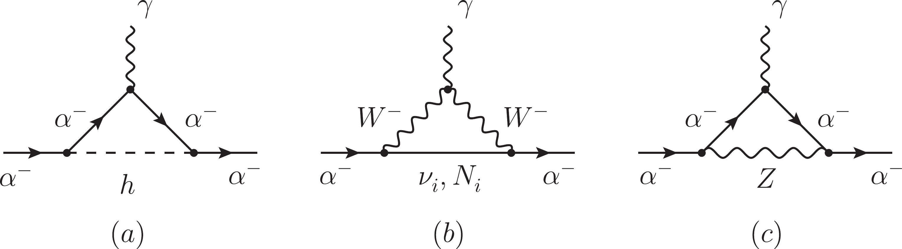
Figure 1. Feynman diagrams for the contributions to the anomalous magnetic moments of the charged lepton
$\alpha^-$ (for$\alpha = e, \mu, \tau$ ) in the type-(I+II) seesaw model: (a) the SM Higgs boson h; (b) the SM charged gauge boson$W^-$ and three light ($\nu^{}_i$ ) or heavy ($N^{}_i$ ) Majorana neutrinos; (c) the SM neutral gauge boson Z.$ \left( {\begin{array}{*{20}{c}} {M_{\rm{L}}^{}}&{M_{\rm{D}}^{}}\\ {M_{\rm{D}}^{\rm{T}}}&{M_{\rm{R}}^{}} \end{array}} \right) = \left( {\begin{array}{*{20}{c}} {\cal{V}}&{\cal{R}}\\ {\cal{S}}&{\cal{U}} \end{array}} \right)\left( {\begin{array}{*{20}{c}} {\hat M_\nu ^{}}&0\\ 0&{\hat M_{\rm{R}}^{}} \end{array}} \right){\left( {\begin{array}{*{20}{c}} {\cal{V}}&{\cal{R}}\\ {\cal{S}}&{\cal{U}} \end{array}} \right)^{\rm{T}}}\;, $

(17) where
$ {\cal{V}} $ ,$ {\cal{R}} $ ,$ {\cal{S}} $ , and$ {\cal{U}} $ are$ 3\times 3 $ non-unitary matrices satisfying the unitarity conditions$ {\cal{V}}{\cal{V}}^\dagger + {\cal{R}}{\cal{R}}^\dagger = {\cal{S}} {\cal{S}}^\dagger + $ $ {\cal{U}} {\cal{U}}^\dagger = {\bf{1}} $ and$ {\cal{V}}{\cal{S}}^\dagger + {\cal{R}}{\cal{U}}^\dagger = {\cal{S}} {\cal{V}}^\dagger + {\cal{U}} {\cal{R}}^\dagger = {\bf{0}} $ . For$ {\cal{O}}(M^{}_{\rm{D}}) $ $ \ll {\cal{O}}(M^{}_{\rm{R}}) $ as in the canonical type-I seesaw model, one can relate the non-unitary matrices$ {\cal{V}} $ and$ {\cal{R}} $ to the unitary matrices V and U introduced in the previous section by$ {\cal{V}} \approx ({\bf{1}} - {\cal{R}} {\cal{R}}^\dagger/2)V $ and$ {\cal{R}} \approx M^{}_{\rm{D}} U^* \widehat{M}^{-1} $ . In the mass basis, the leptonic charged-current interactions read$ {\cal{L}}^{}_{\rm{CC}} = \frac{g}{\sqrt{2}} \overline{\alpha^{}_{\rm{L}}} \gamma^\mu ({\cal{V}}^{}_{\alpha i} \nu^{}_i + {\cal{R}}^{}_{\alpha i} N^{}_i) W^-_\mu + {\rm{h.c.}} \; , $

(18) where
$ \nu^{}_i $ and$ N^{}_i $ (for$ i = 1, 2, 3 $ ) represent the mass eigenfields of three light and heavy Majorana neutrinos, respectively. With the charged-current interactions defined in Eq. (18) and the general formulas derived in Refs. [127, 128], we can obtain the contributions from the light and heavy Majorana neutrinos to the anomalous magnetic moments of the three charged leptons$ a^{W}_\alpha = \frac{G^{}_{\rm{F}} m^2_\alpha}{4 \sqrt{2} \pi^2} \left\{ \mathop \sum \limits_{i = 1}^3 {\cal{V}}^{}_{\alpha i} {\cal{V}}^*_{\alpha i} G\left(\frac{m^2_i}{M^2_W}\right) + \sum^3_{i = 1} {\cal{R}}^{}_{\alpha i} {\cal{R}}^*_{\alpha i} G\left(\frac{M^2_i}{M^2_W}\right) \right\} \; , $

(19) where the loop function is defined as
$ \begin{aligned}[b] G(z) \equiv &\int^1_0 {\rm{d}}x \frac{2x^2 (1+x) + z(2x - 3x^2 + x^3) }{ x + z (1 - x)} \\=& \frac{10 - 43 z + 78 z^2 - 49 z^3 + 4 z^4 + 18 z^3 \ln z}{6(1-z)^4} \; . \end{aligned} $

(20) It is straightforward to verify
$ G(z) = 5/3 - z/2 + {\cal{O}}(z^2) $ in the limit of$ z \ll 1 $ and$ G(z) = 2/3 - (11 - 6\ln z)/ $ $ (2z) + {\cal{O}}(z^{-2}) $ in the limit of$ z \gg 1 $ . The SM value can easily be obtained from Eq. (19) by setting$ {\cal{R}} \to {\bf{0}} $ ,$ {\cal{V}}{\cal{V}}^\dagger \to {\bf{1}} $ , and the vanishing neutrino masses. After subtracting the SM contribution, we obtain the contributions from the massive Majorana neutrinos, i.e.,$ \begin{aligned}[b] \Delta a^{W}_\alpha = &\frac{G^{}_{\rm{F}} m^2_\alpha}{4 \sqrt{2} \pi^2} \left\{ \sum^3_{i = 1} {\cal{R}}^{}_{\alpha i} {\cal{R}}^*_{\alpha i} \left[ G\left(\frac{M^2_i}{M^2_W}\right) - \frac{5}{3}\right] \right.\\&\left.- \frac{1}{2} \sum^3_{i = 1} {\cal{V}}^{}_{\alpha i} {\cal{V}}^*_{\alpha i} \frac{m^2_i}{M^2_W}\right\} \; . \end{aligned} $

(21) It is worthwhile to point out that the loop function in Eq. (20) and the final result in Eq. (21) are different from those in Ref. [129] for the type-I seesaw model. However, the conclusions from Ref. [129] remain valid, namely, the value of
$ [G(M^2_i/M^2_W) - 5/3] $ is always negative and thus$ \Delta a^W_\mu $ has the wrong sign. For illustration, if we consider$ M^{}_i = 1\; {\rm{TeV}} $ (i.e., the limit of$ M^2_i/M^2_W \gg 1 $ holds) and ignore the tiny neutrino masses$ m^{}_i $ , then$ \Delta a^W_\mu \approx -\frac{G^{}_{\rm{F}} m^2_\mu}{4 \sqrt{2} \pi^2} \left({\cal{R}} {\cal{R}}^\dagger\right)^{}_{\mu\mu} \approx - 0.1\times 10^{-11} \; , $

(22) for
$ ({\cal{R}}{\cal{R}}^\dagger)^{}_{\mu\mu} \approx 4.4\times 10^{-4} $ saturating the upper bounds from the electroweak precision data [130]. Compared to the experimental observation given in Eq. (1), the correction from$ \Delta a^W_\mu $ is negligible.Next, we focus on the impact of the triplet Higgs on the anomalous magnetic moment of electron
$ a^{}_e \equiv $ $ (g^{}_e - 2)/2 $ . The latest measurement of the fine structure constant leads to a reevaluation of$ a^{}_e $ , and a$ 1.6\sigma $ discrepancy with the theoretical prediction has been found [131]$ \Delta a^{}_e \equiv a^{\rm{exp}}_e - a^{\rm{SM}}_e = 0.48(30)\times 10^{-12} \; , $

(23) whereas the discrepancy from the caesium recoil measurements is even larger,
$ \Delta a^{}_e \equiv a^{\rm{exp}}_e - a^{\rm{SM}}_e = -0.88(36)\times $ $ 10^{-12} $ with an opposite sign [132]. At the$ 2\sigma $ level, either a positive or negative sign of$ \Delta a^{}_e $ is still allowed, namely,$ \Delta a^{}_e \in [-0.34, 0.98]\times 10^{-12} $ . The result in Eq. (21) is also applicable to the electron case, and it can be estimated by rescaling the value in Eq. (22) by a factor of$ m^2_e/m^2_\mu \approx $ $ 2.368\times 10^{-5} $ . Therefore, the contribution of the massive Majorana neutrinos to$ \Delta a^{}_e $ is negligibly small. In our model, the interaction between the triplet Higgs and charged leptons can be described by$ \begin{aligned}[b] {\cal{L}}^{}_{\rm{Yuk}} =& - \frac{1}{2} y^{}_\Delta \Big[ \sqrt{2} \left( \overline{e^{}_{\rm{L}}} \tau^{\rm{C}}_{\rm{L}} + \overline{\tau^{}_{\rm{L}}} e^{\rm{C}}_{\rm{L}} \right) H^{–} \\& +\left(\overline{\nu^{}_{e{\rm{L}}}} \tau^{\rm{C}}_{\rm{L}} + \overline{\nu^{}_{\tau {\rm{L}}}} e^{\rm{C}}_{\rm{L}} + \overline{e^{}_{\rm{L}}} \nu^{\rm{C}}_{\tau{\rm{L}}} + \overline{\tau^{}_{\rm{L}}} \nu^{\rm{C}}_{e{\rm{L}}} \right) H^- \Big] + {\rm{h.c.}} \; , \end{aligned}$

(24) which induces the corrections to the anomalous magnetic moments of the electron and tauon. The Feynman diagrams in the electron case are shown in Fig. 2, and those in the tauon case can be obtained by exchanging
$ e^- $ and$ \tau^- $ . According to the formulas provided in Ref. [128], the contributions to$ \Delta a^{}_e $ can be calculated as follows: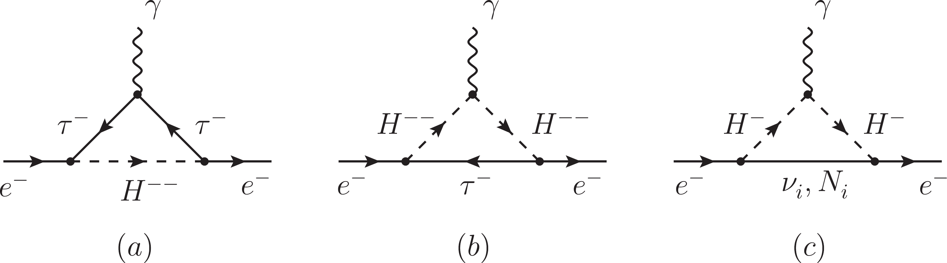
Figure 2. Feynman diagrams for the contributions to the anomalous electron magnetic moment in the type-(I+II) seesaw model: (a) and (b) from the doubly-charged Higgs boson
$H^{--}$ ; and (c) from the singly-charged Higgs boson$H^-$ .$ \begin{aligned}[b] \Delta a^{––}_e =& -\frac{y^2_\Delta m^2_e}{4\pi^2 M^2_\Delta} \int^1_0 {\rm{d}}x \left[\frac{x^2(1 - x)}{x + (m^2_\tau/M^2_\Delta) (1-x)}\right. \\&\left.+ \frac{x^2(1 - x)}{(1 - x) + (m^2_\tau/M^2_\Delta)x} \right] \approx - \frac{y^2_\Delta m^2_e}{12\pi^2 M^2_\Delta} \; , \\ \Delta a^-_e = & -\frac{y^2_\Delta m^2_e}{16\pi^2 M^2_\Delta} \int^1_0 {\rm{d}}x \frac{x^2(1 - x)}{x + (m^2_\tau/M^2_\Delta) (1-x)} \approx - \frac{y^2_\Delta m^2_e}{96\pi^2 M^2_\Delta} \; , \end{aligned} $

(25) where the mass degeneracy of the triplet scalars is assumed and the terms proportional to the small mass ratios
$ m^2_e/M^2_\Delta $ and$ m^2_\tau/M^2_\Delta $ in the integrands have been omitted. The combination of these two contributions gives$ \Delta a^{H}_e = \Delta a^{–}_e + \Delta a^-_e \approx - 3 y^2_\Delta m^2_e/(32\pi^2 M^2_\Delta) $ . Because$ y^{}_\Delta v^{}_\Delta \sim 0.1 $ $ {\rm{eV}} $ , as indicated by the cosmological bound on the sum of the three neutrino masses [133], one obtains$ M^{}_\Delta v^{}_\Delta \sim 26.8 $ $ {\rm{GeV}}\cdot {\rm{eV}} $ to reach the lower bound of the$ 2\sigma $ range, i.e.,$ \Delta a^{}_e = -0.34 \times 10^{-12} $ . At this point, we stress that the doubly-charged Higgs bosons$ H^{\pm \pm} $ and their leptonic decays$ H^{\pm \pm} \to e^\pm \tau^\pm $ can be observed at the CERN Large Hadron Collider. In particular, there exists only one leptonic decay channel$ H^{\pm \pm} \to e^\pm \tau^\pm $ , of which the total decay width is$ \Gamma(H^{\pm \pm} \to e^\pm \tau^\pm) = \frac{y^2_\Delta}{8\pi} M^{}_\Delta \; , $

(26) where the dependence on the triplet Higgs mass
$ M^{}_\Delta $ is different from that in the case of$ \Delta a^{H}_e $ . Therefore, it is interesting to further investigate the determination of the model parameters$ y^{}_\Delta $ ,$ M^{}_\Delta $ , and$ v^{}_\Delta $ by combining the neutrino oscillations, electron magnetic moment, and leptonic decays of the doubly-charged Higgs bosons.Finally, we focus on the anomalous muon magnetic moment, as shown in Fig. 3, to which the dominant contribution is made by the new neutral gauge boson
$ Z^\prime $ . Following the general formulas reported in Refs. [127, 128] and observing the neutral-current interaction shown in Eq. (3), we can calculate the correction from$ Z^\prime $ to$ \Delta a^{}_\mu $ , namely,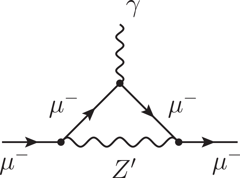
Figure 3. Feynman diagram for the dominant contribution from
$Z^\prime$ to the anomalous muon magnetic moment.$ \Delta a^{Z^\prime}_\mu = \frac{g^2_{Z^\prime} m^2_\mu}{4\pi^2 M^2_{Z^\prime}} \int^1_0 {\rm{d}}x \frac{x^2(1-x)}{(m^2_\mu/M^2_{Z^\prime})x^2 + (1-x)} \approx \frac{g^2_{Z^\prime} m^2_\mu}{12\pi^2 M^2_{Z^\prime}} \; , $

(27) where the term proportional to
$ m^2_\mu/M^2_{Z^\prime} $ has been omitted for$ M^2_{Z^\prime} \gg m^2_\mu $ in the last step. As in our model, the gauge boson$ Z^\prime $ acquires its mass$ M^{}_{Z^\prime} = g^{}_{Z^\prime} v^{}_S/2 $ after the spontaneous symmetry breaking. Therefore, if the anomalous muon magnetic moment$ \Delta a^{}_\mu = 251\times 10^{-11} $ in Eq. (1) is interpreted by the$ Z^\prime $ contribution, then we can identify$ \Delta a^{Z^\prime}_\mu $ with this number and estimate the vev of the singlet scalar from Eq. (27) as$ v^{}_S = \sqrt{\frac{m^2_\mu}{3\pi^2 \Delta a^{Z^\prime}_\mu}} \approx 385\; {\rm{GeV}} \; . $

(28) In the
$ {{U}}(1)_{L^{}_\mu - L^{}_\tau} $ gauge models, for$ M^{}_{Z^\prime} $ around the GeV scale, the most stringent bound has been extracted from the measurement of the neutrino trident events$ \nu^{}_\mu + N \to \nu^{}_\mu + \mu^+ + \mu^- + N $ [134] using the data collected by the CCFR Collaboration [135]. In the mass range$ M^{}_{Z^\prime} \in [0.4, 10^3]\; {\rm{GeV}} $ , the coupling$ g^{}_{Z^\prime} $ favored by the muon$ (g-2) $ has been excluded by the neutrino trident production [134]. However, if$ M^2_{Z^\prime} \ll m^2_\mu $ holds, then the result shown in Eq. (27) will be replaced by$ \Delta a^{Z^\prime}_\mu = \frac{g^2_{Z^\prime}}{8\pi^2} = 203\times 10^{-11} \cdot \left(\frac{g^{}_{Z^\prime}}{4\times 10^{-4}}\right)^2 \; . $

(29) It is evident that the anomalous muon magnetic moment can be entirely explained by choosing
$ g^{}_{Z^\prime} \sim 4\times 10^{-4} $ . For the intermediate range of$ M^{}_{Z^\prime} \lesssim m^{}_\mu $ , the loop integral shown in Eq. (27) varies from$ 0.1 $ for$ m^2_\mu/M^2_{Z^\prime} = 1 $ to$ 1/2 $ for$ m^2_\mu/M^2_{Z^\prime} \gg 1 $ . It can be easily found that$ \Delta a^{Z^\prime}_\mu = 205\times 10^{-11} $ for$ M^{}_{Z^\prime} = 105\; {\rm{MeV}} $ and$ g^{}_{Z^\prime} = 9\times 10^{-4} $ . In this case, we have$ v^{}_S = 2M^{}_{Z^\prime}/g^{}_{Z^\prime} \approx 233\; {\rm{GeV}} $ , which is related to the other model parameters via$ v^{}_\Delta = \lambda^{}_1 v^{}_S v^2_H/M^2_\Delta $ . The constraints on$ M^{}_{Z^\prime} $ at the MeV scale and the gauge coupling$ g^{}_{Z^\prime} $ arise from terrestrial experiments [136-139], astrophysical compact objects [140, 141], and cosmology [142]. However, the parameter space favoring the muon$ (g-2) $ result still survives. -
Motivated by the recent experimental measurement of the anomalous muon magnetic moment, which deviates from the theoretical prediction of the Standard Model at the
$ 4.2\sigma $ level, we proposed an extension of the type-(I+II) seesaw model by the gauged$ L^{}_\mu - L^{}_\tau $ symmetry. By explicitly constructing a viable model with an additional singlet scalar, we demonstrated that the neutral gauge boson$ Z^\prime $ associated with the$ {{U}}(1)^{}_{L^{}_\mu - L^{}_\tau} $ gauge symmetry can possibly help explain the anomalous muon magnetic moment, while the lepton flavor structures are severely constrained as well. The main new results are summarized below.First, for the triplet Higgs ∆ to develop a suitable vacuum expectation value, the introduction of a singlet scalar S with an opposite charge under the
$ {{U}}(1)^{}_{L^{}_\mu - L^{}_\tau} $ symmetry is necessary. At the same time, the mass$ M^{}_{Z^\prime} = g^{}_{Z^\prime} v^{}_S/2 $ of the neutral gauge boson$ Z^\prime $ is essentially determined by the gauge coupling$ g^{}_{Z^\prime} $ and the scale$ v^{}_S $ of spontaneous gauge symmetry breaking. This is distinct from the phenomenological$ Z^\prime $ models, where the gauge-boson mass$ M^{}_{Z^\prime} $ and gauge coupling$ g^{}_{Z^\prime} $ are usually considered to be independent.Second, owing to the new flavor-dependent gauge symmetry, the lepton flavor structures are severely restricted. The charged-lepton and Dirac neutrino Yukawa coupling matrices turn out to be flavor-diagonal. Meanwhile, the leptonic flavor mixing is mainly fixed by the structure of the right-handed neutrino mass matrix, receiving both contributions from the tree-level mass terms and the Yukawa interaction between the right-handed neutrinos and singlet scalar. Interestingly, the effective Majorana mass matrix of three ordinary neutrinos takes the form of the two-zero texture
$ {\boldsymbol{B}}^{}_3 $ , which is compatible with the current neutrino oscillation data at the$ 3\sigma $ level. The predicted strong correlation between the neutrino mass ordering and the octant of$ \theta^{}_{23} $ is readily testable in future neutrino oscillation experiments.Third, we showed that the anomalous magnetic moments of all the three charged leptons receive contributions from the massive Majorana neutrinos, which are, however, found to be negligibly small due to the experimental bounds on the unitarity violation of the leptonic flavor mixing matrix. However, the anomalous electron magnetic moment also acquires corrections from the Higgs triplet, and the correction with a negative sign is obtainable. The anomalous muon magnetic moment can be dominantly explained by the radiative correction from the new neutral gauge boson
$ Z^\prime $ . Considering the present experimental constraints, we find that the parameter space with$ M^{}_{Z^\prime} \sim 100\; {\rm{MeV}} $ and$ g^{}_{Z^\prime} \sim 10^{-4} $ is still allowed.We emphasize that the rich phenomenology of the proposed type-(I+II) model requires further dedicated investigations. The intrinsic correlation among the model parameters can be explored by carefully studying different physical processes, such as neutrino oscillations, lepton-flavor-violating decays of charged leptons, direct searches for new particles at high-energy colliders, and astrophysical and cosmological observations. If the reported discrepancy in the anomalous muon magnetic moment is confirmed by future precision data and refined calculations, it will be definitely intriguing to establish a connection between the possible underlying new physics and the generation of neutrino masses and leptonic flavor mixing. We hope that the results presented in this work will be instructive on this point. The systematic and self-consistent examination of all the phenomenological implications will be conducted in future studies.
-
The author thanks Yu-feng Li and Di Zhang for helpful discussions and Prof. Zhi-zhong Xing for inspiring comments. All the Feynman diagrams included in this work were produced using JaxoDraw [143].
Neutrino masses, leptonic flavor mixing, and muon (g−2) in the seesaw model with the $ {\boldsymbol U(1)^{}_{\boldsymbol L^{}_\mu - \boldsymbol L^{}_\tau} } $ gauge symmetry
- Received Date: 2021-09-06
- Available Online: 2022-01-15
Abstract: The latest measurements of the anomalous muon magnetic moment


 DownLoad: