Generalized Jackiw-Teitelboim gravity in presence of Block brane-like models

I. INTRODUCTION

• I. INTRODUCTION
• II. FORMALISM
• III. LINEAR STABILITY
• IV. SPECIFIC MODELS
•      A Model A
•      B Model B
• V. COMMENTS AND CONCLUSIONS

An interesting way to study quantum effects in gravity is through two-dimensional gravitation. Although this is not a phenomenological description, $2D$ gravity allows for the testing of some conjectures, thereby providing a path for the construction of a quantum theory of gravity in the future. $2D$ gravity has also been used as a theoretical framework to describe complex situations of $4D$ gravity, such as the evaporation of black holes [1–3], dynamics of black holes [4], supergravity [5–7], and other possibilities.

It is known that it is not possible to use the Einstein-Hilbert action for the description of $2D$ gravity, as this leads to identically null equations of motion. In this sense, it becomes necessary to resort to alternative representations to describe two-dimensional gravity. A well known alternative was proposed in the 1980s by Jackiw and Teitelboim, entitled Jackiw-Teitelboim (JT) gravity [8, 9]. In this representation, a real scalar field coupled to gravity, called dilaton field, is used to provide the dynamics of the model. The dilaton field has been used to investigate other physical problems, not only with JT gravity but also through other descriptions; see [10–12].

In order to describe new possibilities, many proposals for generalizing JT gravity have been presented over the years [13–17]. Many of them are motivated by so-called modified theories of gravitation in $4D$, such as $F(R)$-gravity, which introduces a general function of the Ricci scalar in action [18–21], Teleparallel Gravity, in which curvature is replaced by torsion as the mechanism by which geometric deformation produces a gravitational field [22] and also K-fields, which include modifications of the kinematics of the fields [23, 24]. Some generalized gravitation models have proved satisfactory for an attempt to build phenomenologically favorable inflationary models [25–27].

Recently, new theoretical studies have deepened the discussion about the stability of topological solutions in generalized Jackiw-Teilelboim gravity. In Refs. [28, 29] it was shown that it is possible to investigate the linear stability of the solutions by choosing an appropriate gauge. In Ref. [30] it was shown that it is possible to obtain stable solutions for models with unusual dynamics in the form of K-fields, to which cuscuton terms can be introduced to change stability conditions. More recently, in Ref. [31] the authors obtained double-kink solutions using models with standard dynamics.

The key point of these studies was the observation that the result of an analysis of the stability is very similar to the scalar perturbations obtained in five-dimensional braneworld models, which are theories of gravity in which the four-dimensional spacetime is immersed in an extra spatial dimension of infinite extent. This theory was proposed by Randall and Sundrum in 1999 and motivated the development of an alternative explanation for the hierarchy problem [32, 33]. The generalization of the original Randall-Sundrum scenario by incorporating scalar fields was initially proposed in [34–36], and introduced new and interesting perspectives for brane cosmology, such as the study of quintessence [37–39], inflation [40–43] and Teleparallel Gravity [44–46]; see [47–51] for other extended braneworld scenarios.

As $2D$ gravitation has been mirrored in the study of braneworld models, we think it is of interest to understand how the inclusion of new fields of matter can interfere in the study of stability. We know that in braneworld scenarios, when we include new scalar fields as a source of the density Lagrangian, interesting changes can appear in the internal structure of the model. Furthermore, when we include the cuscuton term in Bloch brane models, it seems to induce the appearance of a split in the warp factor [52–55].

Moreover, there is already extensive literature reporting investigations on topological defects in field theories in flat spacetime in the presence of several scalar fields [56–60]. We know that, in these models the study of linear stability is not trivial, because the linearized field equations are, in general, coupled differential equations [61, 62]. Therefore, we think that replicating some considerations of the studies of field theories in flat spacetime, in this new scenario of $2D$ gravity, may also open new research directions for dilaton gravity.

With these motivations in mind, we organize this paper as follows. In Sec. II, we present the general formalism that describes generalized JT gravity in the presence of a dilaton field and also in the presence of coupled scalar matter fields. In Sec. III, we study the linear stability by using the dilaton gauge in the linearized equations of motion. In Sec. IV, we investigate two distinct models that engender kink-like solutions and describe conditions for the emergence of possible bound states. In Sec. V, we present the conclusions and perspectives for future work.

II. FORMALISM

• I. INTRODUCTION
• II. FORMALISM
• III. LINEAR STABILITY
• IV. SPECIFIC MODELS
•      A Model A
•      B Model B
• V. COMMENTS AND CONCLUSIONS

Let us start this investigation by considering a generalization of the Jackiw-Teitelboim gravity that describes two-dimensional gravity in the form

where φ is the dilaton field, κ is a coupling constant, g is the determinant of the metric $g_{\mu\nu}$, $R=g^{\mu\nu}R_{\mu\nu}$ is the Ricci scalar and ${\cal L}_m$ is the Lagrangian density of matter. Here, the greek indexes $\mu,\nu,...$ run from $0$ to $1$ and the fields are all dimensionless.

It is possible to verify that the action defined by Eq. (1) depends on several independent quantities, which are the dilaton field φ, the metric tensor $g_{\mu\nu}$, and in general, the several fields introduced by the Lagrangian density of matter. In this sense, we can derive equations of motion for these quantities by varying the action with respect to them. For example, by variations of the actions with respect to the metric tensor we get the Einstein equation in the form

where $\Box\equiv\nabla_\alpha\nabla^\alpha$ is the two-dimensional Laplacian operator and $T_{\mu\nu}$ is the energy-momentum tensor defined in the usual way as

Note that to obtain the specific form of the energy-momentum tensor we must consider the Lagrangian density ${\cal L}_m$. In this paper, we are interested in investigating models of two scalar fields as matter source fields. With that objective in mind, we will consider a simple Lagrangian density that describes an interaction between the two fields ψ and χ in the form

where $V(\psi,\chi)$ is the potential that governs the interaction of these fields. With this description, we can express the energy-momentum tensor as

See that in addition to the representation giving by the Lagrangian density (4), it is also necessary to specify the form of the potential. Using a variation of Eq. (1) with respect to fields ψ and χ and using the Lagrangian density (4) we get

where we use the indices of V to denote the derivatives of the potential with respect to the matter fields. Similarly, the equation of motion for the dilaton field is obtained by a variation of Eq. (1) with respect to φ, i.e.,

In this case, we then have four independent quantities to consider: the dilaton, the metric tensor and the two scalar fields.

In an attempt to describe solutions with topological behavior, in [28], a two-dimensional representation of the Randall-Sundrum metric used to build five-dimensional braneworld models [33] was considered. We will follow this line and consider a metric in the form

As in the brane models, A is the warp function and ${\rm e}^{2A}$ will also be called warp factor. We assume that it depends only on the spatial coordinate x, i.e., $A=A(x)$. Thus, the Ricci scalar can be written as $R=2A'' +2{A^\prime}^2$, where the prime stands for the derivative with respect to x. Furthermore, we will consider static configurations for the matter fields and for the dilaton field, that is, $\psi=\psi(x)$, $\chi=\chi(x)$ and $\varphi= \varphi(x)$. In this case, the equations of motion (5) become

Note that in general we get coupled equations for the fields ψ and χ as V depends on both fields. Using static configurations, we can also obtain the non-vanishing components of the Einstein equation (2) as

In contrast, the equation of motion for the dilaton field (6) becomes

The five differential equations represented by Eqs. (8), Eqs. (9) and Eq. (10) describe all known information about the system. It is possible to show that one of these equations is not independent and can be obtained from the others, for example, we can use Eqs. (8), (9b) and (10) to obtain Eq. (9a). Thus, the set of five equations can be reduced to four independents equations. This is all we need, as here we have the dilaton φ, the warp function A and the two scalars ψ and χ to be determined.

It was shown in [28] that it is possible obtain a general solution for Eq. (10) in terms of two integration constants. In order to deal with first-order equations we consider a particular solution of Eq. (10) in this paper in the form

To improve the mathematical description, we can use the above solution to rewrite Eqs. (9) as

and

From these two equations it is possible to write the Ricci scalar defined below Eq. (7) in terms of the potential as

Note that, now, we need to work with a system of second-order differential equations that can be solved using the so-called first-order formalism, which allows for a reduction of the second-order differential equations to first-order equations. To proceed with this method, we must introduce an auxiliary function $W(\psi,\chi)$ that correlates the fields ψ and χ such that

where $W_{\psi}=\partial W/\partial \psi$ and $W_{\chi}=\partial W/\partial \chi$. Using the description in Eq. (12) we get the warp function as

Moreover, we can use Eq. (13) to write the potential in the form

The set of first-order equations represented in (15) are commonly found when one studies models described by two scalar fields. See for example [57, 60] in which the authors studied the presence of kink-like solutions in two-dimensional Minkowski spacetime. Also, see [52], in which a system was investigated, which could be described by two real scalar fields coupled with gravity in $(4, 1)$ dimensions in warped spacetime involving one extra dimension. It is worth noting that the first-order Eqs. (15) and (16) solve Eqs. (8) and (9) provided that the potential is given by (17). Furthermore, static and uniform solutions can be obtained from the algebraic equations $W_\psi=0$ and $W_{\chi}=0$, which takes us to a set of points in the space of fields given by $v_i=(\bar\psi_i,\bar\chi_i)$, $i=1,2,\cdots$, which satisfies Eq. (15). Then, we impose that the static solutions $\psi(x)$ and $\chi(x)$ tend to these values when $x\to\pm\infty$.

Due to the asymptotic behavior of the fields, as described above, the function W assumes constant values when the fields $\psi(x)$ and $\chi(x)$ are evaluated at $x\to\pm \infty$, i.e., $W(\psi(x\to\pm\infty), ~ \chi(x\to\pm\infty))=W_{\pm}$. With this, we can use Eq. (16) to write $A(|x| \gg 0)\approx -(\kappa W_\pm/4)\,x$, such that the warp factor ${\rm e}^{2A}$ becomes, asymptotically,

Thus, it may diverge, become a positive constant or vanish, depending on the sign of $W_\pm$ for positive κ .

III. LINEAR STABILITY

• I. INTRODUCTION
• II. FORMALISM
• III. LINEAR STABILITY
• IV. SPECIFIC MODELS
•      A Model A
•      B Model B
• V. COMMENTS AND CONCLUSIONS

In this section, we study the linear stability of dilaton gravitation in the presence of matter fields considering small perturbations around static solutions for the fields. Firstly, let us consider small perturbations in matter fields in the form $\psi\to\psi(x)+\eta(x,t)$ and $\chi\to\chi(x)+\xi(x,t)$. For the dilaton field we write $\varphi\to \varphi(x)+\delta \varphi(x,t)$. Lastly, we consider perturbations with the metric tensor as $g_{\mu\nu}\to g_{\mu\nu}(x)+$ $\pi_{\mu\nu}(x,t)$, where the indices of $\pi_{\mu\nu}$ are raised or lowered as $\pi^{\mu\nu}= -g^{\mu\alpha}\pi_{\alpha\beta}g^{\beta\nu}$.

Using the field perturbations, we can linearize the equations of motion to investigate the linear stability. For example, the $(0,0)$ component of the Einstein equation (2) can be written as

where $V_\psi$ and $V_\chi$ are applied to the static solutions. The $(0,1)$ or $(1,0)$ components are identical and have the form

In contrast, the $(1,1)$ component is

where we used the dot to express the derivative with respect to t and introduced a new variable as

One can show that the linearization of the equations of motion (5) provides us with the relationships,

and

We can also linearize the dilaton equation (6). Here, however, we will follow the description used in [28] and adopt the dilaton gauge, i.e., $\delta \varphi=0$. With this choice, the linearized equation that comes from Eq. (6) vanishes. Furthermore, we can use Eq. (11) to write Eqs. (19) and (21), respectively, as

Let us assume that the perturbations in matter fields can be decomposed as $\eta(x,t)=\sum_n\eta_n(x)\cos(\omega_nt)$ and $\xi(x,t)=\sum_n\xi_n(x)\cos(\omega_nt)$, where $\omega_n$ is a characteristic frequency. Using this decomposition and the set of Eqs. (25), we can represent Eqs. (23) and (24) as

where we defined

and

Note that Eq. (26) is a Sturm-Liouville equation. We can define the inner product of two states as

where $\rho(x)={\rm e}^{-A(x)}$ is the weight function [63, 64]. One can show that Eq. (26) has a state with $\omega=0$, which is given by

where ${\cal N}$ is a normalization constant which can be determined from Eq. (29).

We can use the first-order Eqs. (15), (16) and the potential in the form (17) to rewrite Eq. (26) in terms of the function $W(\psi,\chi)$ as

where we defined

In this case, we can express the stability equation as $S^\dagger S\Upsilon_n=\omega_n^2\Upsilon_n$, where

As in the study on supersymmetric quantum mechanics [65], we can define the supersymmetric partner operator as $SS^\dagger$, and applying it to the state $\Phi_n$, we have

The supersymmetric partner operators $S^\dagger S$ and $SS^\dagger$ can be used to relate their respective eigenstates and eigenvalues, which can facilitate the study of the stability equation (26).

We can also make a change in the variable in the form ${\rm d}z={\rm e}^{-A} {\rm d} x$ in order to make the metric conformally flat; in this case, the stability equation (26) becomes a Schrödinger-like equation, i.e.,

where

Here, we are using the index z to represent the derivative with respect to the new variable z, as in $\psi_z={\rm d}\psi/{\rm d}z$, etc. We also have a state with $\omega=0$, that is

Similarly to the Sturm-Liouville equation, we can fatorize Eq. (35) into ${\cal S}^\dagger {\cal S}\,\Upsilon_n=\omega_n^2\Upsilon_n$. Here, the operator ${\cal S}$ is given by

As we see, it is possible to study the linear stability of static solutions through a Schrödinger-like equation. In this case, to determine the correspondence between the two variables x and z, one has to integrate to find x as a function of z. However, this change cannot always be done analytically. Therefore, it is necessary to resort to numerical methods, as we will illustrate in one of our examples.

We can see from Eq. (37) that the zero mode may be divergent for $A_z=0$, and that this may lead to a non normalized zero mode. As the derivative of the warp function is proportional to W (see Eq. (16)), we can analyze the asymptotic behavior of W to get further insight into the behavior of the zero mode. We know that $W\to W_{\pm}$ asymptotically, so if the sign of $W_-$ is different from the sign of $W_+$, W has to vanish somewhere along the z axis to obstruct the normalization of the zero mode. In this sense, to make the zero mode normalizable, the sign of W should not change, and the warp factor should not diverge asymptotically.

IV. SPECIFIC MODELS

• I. INTRODUCTION
• II. FORMALISM
• III. LINEAR STABILITY
• IV. SPECIFIC MODELS
•      A Model A
•      B Model B
• V. COMMENTS AND CONCLUSIONS

In this section, we study two distinct models in order to understand how the formalism presented so far works. Furthermore, we investigate how the matter fields interact and give rise to the dilaton field, the warp factor and the Ricci scalar.

A Model A

• I. INTRODUCTION
• II. FORMALISM
• III. LINEAR STABILITY
• IV. SPECIFIC MODELS
•      A Model A
•      B Model B
• V. COMMENTS AND CONCLUSIONS

The first model that we consider in this paper is motivated by the so-called Bloch brane, which is a five-dimension braneworld model constructed by the interaction of two real scalar fields. The model was first considered in [52], in which the authors used an auxiliary function $W(\psi,\chi)$, to which we now add a real constant c to get

where r is a real parameter. In particular, c can be used to modify the structure of the solutions and r is positive and controls the coupling between the fields. Using the algebraic equations, $W_\chi=0$ and $W_\psi=0$, we obtain four sets of values for the asymptotic behavior of the fields: $v_{1}=(1,0)$, $v_{2}=(-1,0)$, $v_{3}=(0,1/\sqrt{r})$ and $v_{4}=(0,-1/\sqrt{r})$. Therefore, the auxiliary function W assumes the values, $W(v_{1}) = c+ 2/3$, $W(v_{2}) = c-2/3$ and $W(v_{3}) = W(v_{4}) = c$.

We can then obtain the asymptotic behavior of the warp factor using the asymptotic behavior of the fields. For example, for the solutions that connect $v_2$ to $v_1$, we get

where the plus sign in the exponential is for $x\to\infty$ and the minus sign for $x \to -\infty$. Note that, the warp factor has an asymmetric behavior when $c \neq 0$; furthermore, it tends asymptotically to zero at both extremes if $|c| < 2/3$, however, if $|c| > 2/3$ the warp factor diverges at one side. In contrast, the solutions that connect the values $v_4$ and $v_3$, lead to

In this case, the warp factor is asymmetric and not localized anymore. Using the model defined in (39), we can obtain the interaction potential of the matter fields as

Using the asymptotic values of the solutions, we find that $V(\pm1,0) = -(\kappa/8)(c \pm 2/3)^2$ and $V(0,\pm 1/\sqrt{r}) = -\kappa c^2/8$. Note that, for $\kappa>0$, we have $V(\bar{\psi}_i,\bar{\chi}_i)\leq0$ in all cases; this indicates that the space can be $AdS_2$ or $M_2$ asymptotically depending on the value of parameter c. As mentioned below Eq. (13), it is possible to relate the potential with the Ricci scalar. This result is interesting because it is possible to calculate the asymptotic value of the Ricci scalar directly without knowing the solutions in their explicit form, using only the required boundary conditions, as we will implement below.

We can now investigate the specific solutions of the model. For this, we use Eq. (15) to obtain a system of first-order differential equations as

We can solve the set of coupled differential equations in Eq. (43) numerically aiming to obtain solutions that connect the values $v_i$ obtained by solving the algebraic equations. However, it was shown in [58] that it is possible to decouple this system of equations considering the orbits $F(\psi,\chi)=0$ that connect the uniform solutions $v_i$. For this model we have orbits in the form

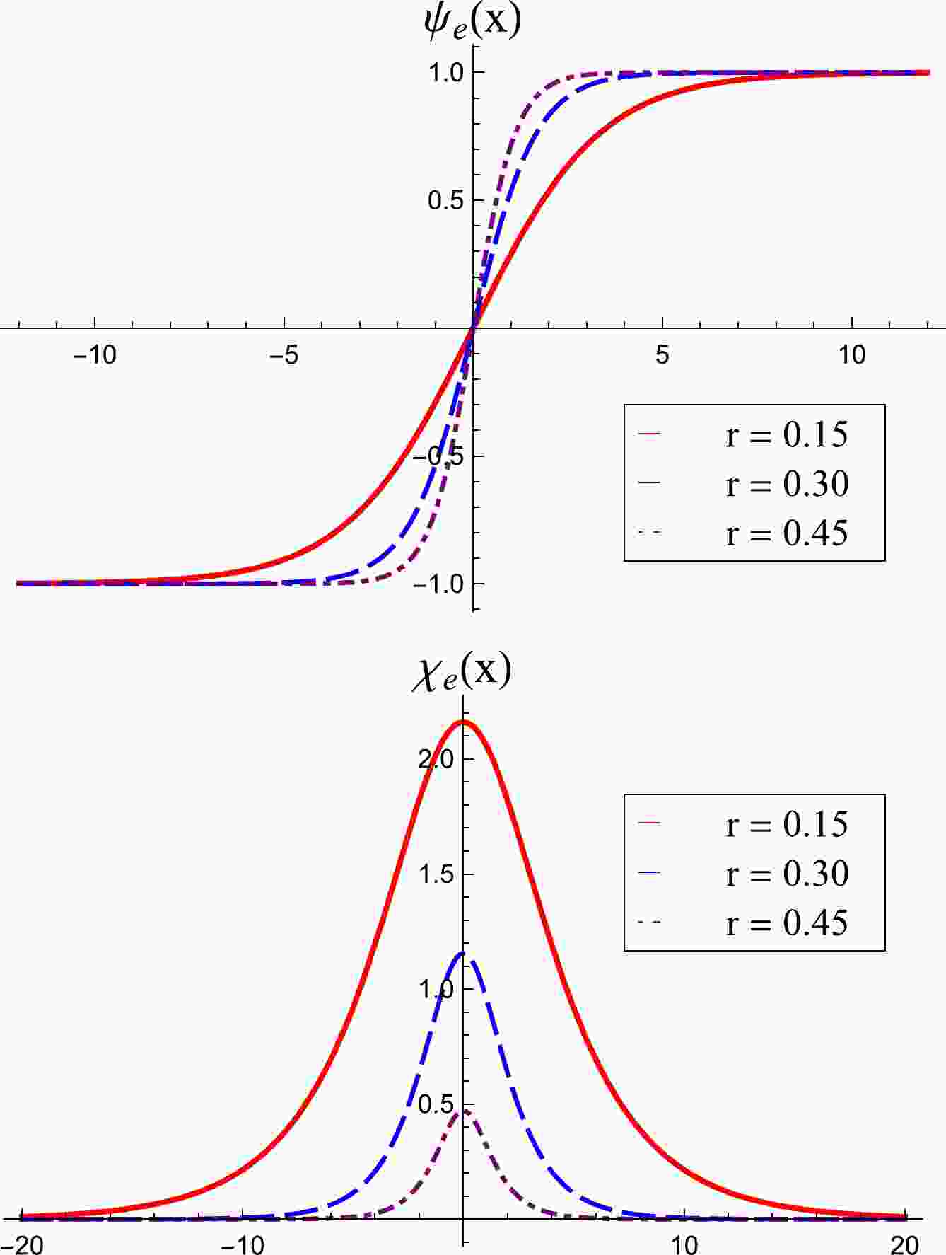
where b is a real integration constant that controls the shape of the above orbits. Here, we consider $b=0$. There is an interesting orbit, which is an elliptical one; in this case we have the solution

with $r\in (0, 1/2]$. The parameter r controls the thickness of the solutions and the height of $\chi_e(x)$, as can be seen in Fig. 1, where we display the above solutions for $r=0.15$, $0.30$ and $0.45$. We can show that, for $r\to 1/2$, the orbit becomes a straight line, with the solution

Figure 1

Figure 1.  (color online) Solutions for the elliptic orbit represent by Eq. (45a) (top panel) and Eq. (45b) (bottom panel).

DownLoad: Full-Size Img PowerPoint

Using Eqs. (16) and (11), we can obtain the dilaton field solution for the different possible orbits. For example, for the straight orbit we get

In contrast, for the elliptic orbit we have

Moreover, Fig. 2 shows the behavior of the dilaton field solution obtained by previous equations and depicted for $\kappa=1$, $r=1/4$ (elliptical orbit), and $c=0,\,1/3, \,2/3,\,1$.

Figure 2

Figure 2.  (color online) Dilaton field for straight orbit (top panel) and elliptic orbit (bottom panel) with $\kappa=1$ and $r=1/4$.

DownLoad: Full-Size Img PowerPoint

We also study the warp factor, and the two panels in Fig. 3 show how it behaves for the straight orbit (top panel) and for the elliptic orbit (bottom panel) with $r=1/4$.

Figure 3

Figure 3.  (color online) Warp factor for straight orbit (top panel) and for elliptic orbit (bottom panel) with $\kappa=1$ and $r=1/4$.

DownLoad: Full-Size Img PowerPoint

We can also calculate the Ricci scalar to verify how it behaves for the orbits obtained above. Using Eq. (14) and the potential in Eq. (42), the Ricci scalar can be obtained; for the straight orbit we get

However, in the case of the elliptic orbit we obtain

Figure 4 shows the Ricci scalar for the two orbits obtained here. We used $\kappa=1$, $c=0,1/3,2/3,1$ and for the elliptic orbits, $r=1/4$. For both, the straight and elliptic orbits, we have $R(x \to \pm \infty) = (\kappa^2/72)(2\pm3c)^2$, as calculated below Eq. (42). As we can see, the Ricci scalar is asymptotically constant, indicating that the two-dimensional space can be $M_2$ or $AdS_2$, see Ref. [66] for more details.

Figure 4

Figure 4.  (color online) Ricci scalar for straight orbit (top panel) and for elliptic orbit (bottom panel) with $\kappa=1$ and $r=1/4$.

DownLoad: Full-Size Img PowerPoint

Now, we turn our attention to investigating the linear stability of the solutions. We begin by analyzing the stability of the solutions for the straight orbit given by Eq. (46). In this case, the component $q(x)$ of Eqs. (28) vanishes, i.e., $q(x)=0$. Thus, the equations of stability (26) become two independent equations. In this case, we can examine each perturbation separately, i.e.,

where

and we defined $W_s(x)=c+\tanh(x)-(1/3)\tanh^3(x)$. We can use Eq. (51a) to obtain the zero mode as

where ${\cal N}$ is a normalization constant that can be obtained with Eq. (29). It is possible to verify that the zero mode is only normalizable for $c>2/3$. This integration can be done numerically, for example, for $\kappa = c = 1$, we have ${\cal N}\approx 0.668$. Using the supersymmetric partner equation in (34), it is possible to show that there is no normalizable eigenstate, regardless of the value of c. Thus, the stability equation (51a) will only have the eigenvalue $\omega_0=0$ with the eigenstate given by (53).

Let us now analyze Eq. (51b). In this case, the mode-zero is given by

where $\tilde{ {\cal N}}$ is another normalization constant. In this case, we find that the zero mode is always normalizable, regardless of the value of the parameter c. For instance, taking $\kappa=1$ and $c=0$, $1/3$, $2/3$ and $1$, we obtain $\tilde{ {\cal N}}\approx 0.683$, $0.682$, $0.679$ and $0.673$, respectively. We also verify that the zero mode is the only eigenstate present in this case.

We can change variables from x to z, as ${\rm d}z={\rm e}^{-A}{\rm d}x$, so that the Eqs. (51) become Schrödinger-like equations of the form

where the potentials are defined as ${\cal U}_1(z)={\rm e}^{2A(z)}p(z)$ and ${\cal U}_2(z)={\rm e}^{2A(z)}\bar{p}(z)$, and $A(z)=\varphi(z)/2$ is obtained by Eq. (47). In Fig. 5 we show the behavior of the potentials ${\cal U}_1(z)$ and ${\cal U}_2(z)$ for $\kappa=1$ and c as in Fig. 2. This result is numerical because it is not possible to change the variable from x to z analytically. It is possible to show that the potential ${\cal U}_1(z)$ supports the zero mode if $2/3<c<2(12+\kappa)/ (3\kappa)$. This result is in accordance with the investigation presented in Ref. [28]. For the second field there is the potential ${\cal U}_2(z)$ which is a result of the perturbation around the corresponding solution. In this case, it is possible to obtain the zero mode if $2/3<c< 2(6+\kappa)/(3\kappa)$, as can be seen in the bottom panel of Fig. 5.

Figure 5

Figure 5.  (color online) Plot of the stability potentials ${\cal U}_1(z)$ (top panel) and ${\cal U}_2(z)$ (bottom panel) for the straight orbit using $\kappa=1$.

DownLoad: Full-Size Img PowerPoint

To study the stability for the elliptical orbit, we first notice that $q(x)\neq0$, and the system of Eqs. (26) no longer decouples. In this case, we must deal with a matrix representation of the equations. As the expressions of $p(x)$, ${\bar p}(x)$ and $q(x)$ in Eq. (26) are long and awkward, we first define the quantities $T(x)=\tanh(2rx)$, $S(x)= \rm{sech}(2rx)$ and

and now the components of Eq. (28) can be worked out to be written in the following form

In this case, the zero mode can be obtained by Eq. (30) in the form

where ${\cal N}$ is the normalization constant determined by Eq. (29), and in order to have normalized states, we need to assume that $c>2/3$.

B Model B

• I. INTRODUCTION
• II. FORMALISM
• III. LINEAR STABILITY
• IV. SPECIFIC MODELS
•      A Model A
•      B Model B
• V. COMMENTS AND CONCLUSIONS

Let us now consider another model for which we obtain kink-like solutions. For this, we assume that

where, in addition to the real constant c, we also introduce two new real parameters $\gamma_1$ and $\gamma_2$ that influence the thickness of the solutions. It is interesting to note that although Eq. (59) does not contain interactions between fields explicitly, we still have a system whose potential $V(\psi,\chi)$ is coupled. This can be easily verified by Eq. (17), whose term $W^2$ provides the interaction between the two fields. This possibility was also considered in Refs. [67–69] in the braneworld context in five-dimensional spacetime with an extra spatial dimension of infinite extent. In the present case, the potential becomes

The asymptotic values of the solutions of model (59) can also be obtained by algebraic equations in the form $W_\psi=0$ and $W_\chi=0$. In this case, we have $v_{\pm}=(1,\pm1)$ and $\bar{v}_{\pm}=(-1,\pm1)$. Thus, $W(v_{\pm}) \equiv W_{\pm} = c+2\gamma_1/3\pm2\gamma_2/3$ and $W(\bar{v}_{\pm})\equiv \bar{W}_{\pm}=c-2\gamma_1/3\pm2\gamma_2/3$. Using the asymptotic values of the solutions for the potential, we obtain $V(v_{\pm})= -\kappa W_{\pm}^2/8$ and $V(\bar{v}_{\pm})=-\kappa \bar{W}_{\pm}^2/8$.

Let us now obtain the solutions for this model. We can write the first-order equations (15) as

The above first-order equations allow for kink-like solutions in the form:

where $x_0$ and $\tilde{x}_0$ are real constants that define the center of the solutions, while the parameters $\gamma_1$ and $\gamma_2$ control their thickness. We can also find the dilaton field using Eqs. (16) and (11) to write

As we know it is possible to calculate the warp factor of this model from the above equation as ${\rm e}^{2A(x)}$. Let us now turn our attention to how the parameters c, $\gamma_1$, $\gamma_2$, ${x}_0$, and $\tilde{x}_0$ modify the dilaton field and the warp factor. Firstly, we consider $c=0$, $\gamma_1=\gamma_2$, and $\tilde{x}_0=-x_0$; in this case, the parameter $x_0$ enlarges the center of the dilaton and the warp factor. This behavior can be seen in Fig. 6, in which we display $\varphi(x)$ and ${\rm e}^{2A(x)}$, for $c=0$, $\kappa= \gamma_1=\gamma_2=1$, and $x_0=0$, $2.5$, $5$ and $7.5$. In the previous model, the parameter c was responsible for an asymmetry in the dilaton field and warp factor; however, in the present model, we can generate an asymmetry from the parameters $\gamma_1$ and $\gamma_2$. To see this, we consider Fig. 7, where $c=0$, $\kappa= \gamma_1=1$, and $x_0=-\tilde{x}_0=5$ with $\gamma_2=1$, $1.1$, $1.2$, and $1.3$. As can be observed, it is possible to obtain asymmetric quantities with the parameter $c=0$. This is interesting because the model allows the warp factor to be always localized. Nevertheless, it is also possible to obtain asymmetric quantities through the parameter c. However, depending on the value of c, this may lead to a delocalized warp factor. In addition, the parameter c works differently from $\gamma_1$ and $\gamma_2$ in producing asymmetries; therefore, it is not possible for them to cancel each other's effects.

Figure 6

Figure 6.  (color online) Dilaton field and warp factor plotted for $c=0$, $\kappa=1$, $\gamma_1=\gamma_2=1$ and $\tilde{x}_0=-x_0$.

DownLoad: Full-Size Img PowerPoint

Figure 7

Figure 7.  (color online) Dilaton field and warp factor plotted for $c=0$, $\kappa=\gamma_1=1$ and $x_0=-\tilde{x}_0=5$.

DownLoad: Full-Size Img PowerPoint

To better understand the asymptotic behavior of gravity we can calculate the Ricci scalar. In the present case we have:

It is possible to show that

This result shows that the Ricci scalar tends to a non negative constant asymptotically, whereby the parameter c also generates an asymmetry in this case. In Fig. 8 we depict the Ricci scalar for some values of the parameters. In the top panel, we use $c=0$, $\kappa=\gamma_1=\gamma_2=1$, $\tilde{x}_0=-x_0$ with $x_0$ as in Fig. 6. In the bottom panel, we use $c=0$, $\kappa=\gamma_1=1$, $x_0=-\tilde{x}_0=5$ and $\gamma_2$ as in Fig. 7.

Figure 8

Figure 8.  (color online) Top panel shows the Ricci scalar depicted for $c=0$, $\kappa=\gamma_1=\gamma_2=1$ and $\tilde{x}_0=-x_0$. Bottom panel shows the Ricci scalar depicted for $c=0$, $\kappa=\gamma_1=1$ and $x_0=$$-\tilde{x}_0=5$.

DownLoad: Full-Size Img PowerPoint

Again, a study of stability is implemented via the matrix Eq. (26), with the components (28), which in this case can be written as:

where $T_1(x) = \tanh\big(\gamma_1(x - x_0)\big)$, $T_2(x) = \tanh\big(\gamma_2(x - \tilde{x}_0)\big)$, $S_1(x)= \rm{sech}\big(\gamma_1(x - x_0)\big)$, $S_2(x)= \rm{sech}(\gamma_2\big(x - \tilde{x}_0)\big)$ and

Again, we can calculate the zero mode in the following form

where the normalization constant ${\cal N}$ can be obtained using Eq. (29).

V. COMMENTS AND CONCLUSIONS

• I. INTRODUCTION
• II. FORMALISM
• III. LINEAR STABILITY
• IV. SPECIFIC MODELS
•      A Model A
•      B Model B
• V. COMMENTS AND CONCLUSIONS

In this study, we investigated two-dimensional Jackiw-Teitelboim gravity, in which the Lagrange density of matter displays coupled scalar fields. We investigated models that appeared before in studies of the five-dimensional braneworld model and considered two specific situations for which it is possible to obtain topological solutions to the matter fields analytically. For each case, we obtained the solution of the dilaton field and analyzed the linear stability. We verified that, in general, the equations of stability for the matter fields are coupled, obtained in the matrix form.

In the first model, we investigated the analogous situation of the so-called Bloch brane that was studied in [52]. We verified that it is possible to obtain a set of solutions for the matter fields that present topological behavior and connect the asymptotic values obtained by the algebraic equations $W_\psi=0$ and $W_\chi=0$; however, the result is generally non-analytical. Nevertheless, for an adequate choice of parameters, it is possible to obtain two classes of analytical solutions that describe straight and elliptic orbits. For these two specific situations, we found the dilaton field solution and showed that the Ricci scalar presents the usual behavior, connecting two asymptotic $AdS_2$ or $M_2$ spaces. Although the general solutions only allow us to reconstruct the stability potential in the matrix form, we found that for the specific case of the straight orbit, the equations of the perturbations were decoupled, and we could analyze each perturbation of the matter fields separately.

In the second model studied in this paper, we used an auxiliary function that generates kink solutions with different thicknesses. We showed that even though the coupling of the fields is not present in the auxiliary function, the scalar potential is still coupled. We also obtained the solution for the dilaton field and verified the behavior of the Ricci scalar. Moreover, we studied the stability in the matrix representation as the equations of stability do not decouple. However, we found the zero mode analytically.

In addition to the study presented here, we think it is also of current interest to address situations in which JT gravity is generalized by introducing new scalars built from the Ricci scalar, such as in $\,F(R)$-gravity [18–21], and models with gauge and other fields. Another direction of current interest concerns the study of 2D Einstein-Maxwell-Dilaton gravity and connections with $AdS_2$ holography; see, e.g., Ref. [70] and references therein for further details on this subject. Furthermore, modifications that aim to encompass exotic properties such as dark matter and dark energy were obtained through the inclusion of matter fields with unusual dynamics, called K-fields [23, 24]. We are also studying dilaton gravity [12] with the inclusion of fields that engender compact behavior. We believe that new studies along the above lines may add other effects and give rise to new research perspectives for $2D$ gravity. These and other related issues are now under consideration, and we hope to report on them in the near future.

References