Decay constants of B_c(nS) and ${\boldsymbol B_c^*}$ (nS)

I. INTRODUCTION

• I. INTRODUCTION
• II. MODEL
• III. DECAY CONSTANT
• IV. RESULTS
• V. SUMMARY AND CONCLUSION
• ACKNOWLEDGEMENTS
• APPENDIX A
• APPENDIX B

$B_c$ mesons are the only open flavor mesons containing two heavy valence quarks, i.e. one charm quark and one bottom anti-quark (or vice versa). The flavor forbids their annihilation into gluons or photons, so the ground state pseudoscalar $B_c(1S)$ can only decay weakly, which makes it particularly interesting for the study of the weak interaction. From an experimental aspect, $B_c$ mesons are much less explored than charmonium and bottomonium due to their small production rate, as the dominant production mechanism requires the production of both $c\overline{c}$ and $b\overline{b}$ pairs. The $B_c(1S)$ meson was first observed by CDF experiment in 1998 [1]. In later years, the mass and lifetime of $B_c(1S)$ were measured precisely, and its hadronic decay modes were also observed [2–5]. The excited $B_c$ meson state was not observed until 2014 by the ATLAS experiment [6]. The mass of $B_c(2S)$ was measured by the LHCb experiment [7] and CMS experiment [8] independently in 2019. However, for the vector $B_c$ mesons, only the mass difference $M_{B_c^*(2S)} - M_{B_c^*(1S)} = 567\ {\rm{ MeV}}$ is known [8].

From a theoretical aspect, the mass spectrum and the decays of $B_c$ mesons are investigated by various methods; for example, the quark model [9–14], the light-front quark model [15–17], the QCD sum rule [18–20], the QCD factorization [17,21–24], the instantaneous approximation Bethe-Salpeter equation [25, 26], the continuum QCD approach [27–29], the lattice QCD [30] and other methods [31–33]. The quark model, with the interaction motivated by quantum chromodynamics (QCD), is quite successful in describing the hadron spectrum and decay branching ratios; see Refs. [34, 35] for an introduction. The nonrelativistic version of the quark model is suitable for heavy quark systems. It is not only phenomenologically successful in describing mesons and baryons [36–38] but also powerful in predicting the properties of exotic hadrons, such as tetraquarks [39, 40].

The decay constant carries information of the strong interaction in leptonic decay, and thus it is intrinsically nonperturbative. A precise determination of the decay constant is crucial for a precise calculation of the leptonic decay width. In this paper, we investigate the decay constants of low lying S-wave $B_c$ mesons, i.e. $B_c(nS)$ and $B^*_c(nS)$ with $n\leq 3$ in the nonrelativistic quark model. As $B_c$ mesons are less explored, our result is significant for both theoretical and experimental exploration of the $B_c$ family. The work of Lakhina and Swanson [41] showed that two elements are important in calculating decay constants within the nonrelativistic quark model: one is the running coupling of the strong interaction, and the other is the relativistic correction. Both of these elements are taken into account in this paper. Moreover, the uncertainty due to varying parameters and losing Lorentz covariance are considered carefully.

This paper is organized as follows. In section II, we introduce the framework of the quark model. The formulas for the decay constants in the quark model are given in section III. In section IV, the results of mass spectrum and decay constants are presented and discussed. A summary and conclusions are given in section V. We also present the mass spectrum and decay constants of charmonium in Appendix A and those of bottomium in Appendix B for comparison.

II. MODEL

• I. INTRODUCTION
• II. MODEL
• III. DECAY CONSTANT
• IV. RESULTS
• V. SUMMARY AND CONCLUSION
• ACKNOWLEDGEMENTS
• APPENDIX A
• APPENDIX B

The framework has been introduced elsewhere; see for example Refs. [10, 36, 37]. We recapitulate the framework here for completeness and to specify the details. The masses and wave functions are obtained by solving the radial Schrödinger equation,

where $T =- \dfrac{\hbar^2}{2\mu_m r^2}\dfrac{{\rm{d}}}{{\rm{d}}r}\left(r^2\dfrac{{\rm{d}}}{{\rm{d}}r}\right) + \dfrac{L(L+1)\hbar^2}{2\mu_m r^2}$ is the kinetic energy operator, r is the distance between the two constituent quarks, $R(r)$ is the radial wave function, $\mu_m = \dfrac{m \bar{m}}{m + \bar{m}}$ is the reduced mass with m and $\bar{m}$ being the constituent quark masses, and L is the orbital angular moment quantum number. V is the potential between the quarks and E is the energy of this system. The meson mass is then $M = m + \bar{m} + E$. Note that the complete wave function is $\Phi_{nLM_L}({\boldsymbol{r}}) = R_{nL}(r)Y_{LM_L}(\theta,\phi)$, where n is the main quantum number, $M_L$ is the magnetic quantum number of orbital angular momentum, and $Y_{LM_L}(\theta,\phi)$ is the spherical harmonics. In this paper a bold character stands for a three-dimensional vector, for example, ${\boldsymbol{r}} = \vec{r}$.

The potential could be decomposed into

$H^{{\rm{SI}}}$ is the spin independent part, which is composed of a coulombic potential and a linear potential,

where b is a constant and $\alpha_s(Q^2)$ is the running coupling of the strong interaction. The other three terms are spin dependent.

is the spin-spin contact hyperfine potential, where ${\boldsymbol{s}}$ and ${\boldsymbol{\bar{s}}}$ are the spin of the quark and antiquark respectively, and $\tilde{\delta}_\sigma({\boldsymbol{r}}) = \left(\dfrac{\sigma}{\sqrt{\pi}}\right)^3 {\rm{e}}^{-\sigma^2 r^2}$ with σ being a parameter.

is the tensor potential. $H^{{\rm{SO}}}$ is the spin-orbital interaction potential and could be decomposed into a symmetric part $H^{{\rm{SO+}}}$ and an anti-symmetric part $H^{{\rm{SO-}}}$, i.e.

where ${\boldsymbol{S}}_\pm = {\boldsymbol{s}} \pm {\boldsymbol{\bar{s}}}$, and ${\boldsymbol{L}}$ is the orbital angular momentum of the quark and antiquark system.

In Eqs. (3)$-$(8), the running coupling takes the following form:

where $\Lambda_{{\rm{QCD}}}$ is the energy scale below which nonperturbative effects take over, $\beta = 11-\dfrac{2}{3}N_f$ with $N_f$ being the flavor number, Q is the typical momentum of the system, and $\alpha_0$ is a constant. Equation (9) approaches the one loop running form of QCD at large $Q^2$ and saturates at low $Q^2$. In practice $\alpha_s(Q^2)$ is parametrized by the form of a sum of Gaussian functions and transformed into $\alpha_s(r)$ as in Ref. [35].

It should be mentioned that the potential containing $\dfrac{1}{r^3}$ is divergent. Following Refs. [36, 37], a cutoff $r_c$ is introduced, so that $\dfrac{1}{r^3} \to \dfrac{1}{r^3_c}$ for $r \leq r_c$. Herein $r_c$ is a parameter to be fixed by observables. Most of the interaction operators in Eq. (2) are diagonal in the space with basis $|JM_J;LS \rangle$ except $H^{{\rm{SO-}}}$ and $H^{{\rm{T}}}$, where J, L and S are the total, orbital and spin angular momentum quantum numbers, and $M_J$ is the magnetic quantum number. The anti-symmetric part of the spin-orbital interaction, $H^{{\rm{SO-}}}$, arising only when the quark masses are unequal, causes $^3L_J \leftrightarrow ^1L_J$ mixing. The tensor interaction, $H^{{\rm{T}}}$, causes $^3L_J \leftrightarrow ^3L'_J$ mixing. The former mixing is considered in our calculation while the latter one is ignored, as the mixing due to the tensor interaction is very weak [35].

There are eight parameters in all: m, $\bar{m}$, $N_f$, $\Lambda_{{\rm{QCD}}}$, $\alpha_0$, b, σ and $r_c$. m and $\bar{m}$ are fixed by the mass spectra of charmonium and bottomium; see Appendix A and Appendix B. $N_f$ and $\Lambda_{{\rm{QCD}}}$ are chosen according to QCD estimation. $N_f=4$ for charmonium and $B_c$ mesons, and $N_f = 5$ for bottomium mesons. In this work we vary $\Lambda_{{\rm{QCD}}}$ in the range $0.2 {\rm{ GeV}} <\Lambda_{{\rm{QCD}}} < 0.4{\rm{ GeV}}$, and $\alpha_0$, b, σ and $r_c$ are fixed by the masses of $B_c(1^1S_0)$, $B_c(2^1S_0)$, $B^*_c(1^3S_1)$ and $B_c(1^3P_0)$. For the $B_c$ meson masses, the experimental values [42] or the lattice QCD results [30] are referred.

III. DECAY CONSTANT

• I. INTRODUCTION
• II. MODEL
• III. DECAY CONSTANT
• IV. RESULTS
• V. SUMMARY AND CONCLUSION
• ACKNOWLEDGEMENTS
• APPENDIX A
• APPENDIX B

The decay constant of a pseudoscalar meson, $f_P$, is defined by

where $|P(p) \rangle$ is the pseudoscalar meson state, $p^\mu$ is the meson four-momentum, and $j^{\mu 5}(x) = \bar{\psi}\gamma^\mu \gamma^5 \psi(x)$ is the axial vector current with $\psi(x)$ being the quark field. In the quark model the pseudoscalar meson state is described by

where ${\boldsymbol{k}}$, ${\boldsymbol{\bar{k}}}$ and ${\boldsymbol{p}}$ are the momenta of the quark, antiquark and meson respectively, $E_p =\sqrt{M^2 + {\boldsymbol{p}}^2}$ is the meson energy, $N_c$ is the color number, ${\boldsymbol{S}}(={\boldsymbol{S}}_+)$ is the total spin and ${\boldsymbol{M_S}}$ is its z-projection (in the case of pseudoscalar meson, ${\boldsymbol{S}} = {\boldsymbol{M_S}} = 0$), and $b^\dagger_{{\boldsymbol{ks}}}$ and $d^\dagger_{{\boldsymbol{\bar{k}\bar{s}}}}$ are the creation operators of the quark and antiquark respectively. $\chi^{{\boldsymbol{SM_S}}}_{{\boldsymbol{s\bar{s}}}}$ is the spin wave function, and $\Phi\left(\dfrac{\bar{m}{\boldsymbol{k}} - m{\boldsymbol{\bar{k}}}}{m+\bar{m}} = {\boldsymbol{k}}_r\right)$ is the wave function in momentum space, where ${\boldsymbol{k}}_r$ is the relative momentum between the quark and antiquark. While $\Phi({\boldsymbol{k}}_r) = \int {\rm{d}}^3{\boldsymbol{r}}\Phi({\boldsymbol{r}}) {\rm{e}}^{-{\rm i}{\boldsymbol{k}}_r \cdot{\boldsymbol{r}}}$, we use the same symbol for wave functions in coordinate space and momentum space.

The decay constant is Lorentz invariant by definition, as in Eq. (10). However, $|P(p) \rangle$ defined by Eq. (11) is not Lorentz covariant, and thus leads to ambiguity about the decay constant. Letting the four-momentum be $p^\mu = (E_p, {\boldsymbol{p}})$ and ${\boldsymbol{p}} = (0,0,p)$, we can obtain the decay constant by comparing the temporal ($\mu = 0$) component or the spatial ($\mu = 3$) component of Eq. (10). The decay constant obtained with the temporal component is

where ${\boldsymbol{l}}_+ = {\boldsymbol{l}} + \dfrac{m{\boldsymbol{p}}}{m+\bar{m}}$, ${\boldsymbol{l}}_- = {\boldsymbol{l}} - \dfrac{\bar{m}{\boldsymbol{p}}}{m+\bar{m}}$, $E_{l_+} = \sqrt{({\boldsymbol{l}}_+)^2 + m^2}$, and $\bar{E}_{l_-} = \sqrt{({\boldsymbol{l}}_-)^2 + \bar{m}^2}$. The decay constant obtained with the spatial component is

The Lorentz covariance is violated in two aspects. Firstly, Eqs. (12) and (13) lead to different results. Secondly, $f_P$ varies as the momentum $p = |{\boldsymbol{p}}|$ varies. Losing Lorentz covariance is a deficiency of nonrelativistic quark model and covariance is only recovered in the nonrelativistic and weak coupling limits [41]. Herein we treat the center value as the prediction, and the deviation is treated as the uncertainty due to losing Lorentz covariance.

The decay constant of a vector meson, $f_V$, is defined by

where $M_V$ is the vector meson mass, $\epsilon^\mu$ is its polarization vector, $j^{\mu}(x) = \bar{\psi}\gamma^\mu \psi(x)$ is the vector current, the vector meson state is the same as Eq. (11) except ${\boldsymbol{S}} = 1$ and ${\boldsymbol{M_S}} = 0, \pm 1$ (we use the quantum number to present the value of the angular momentum). With $p^\mu = (E_p, 0,0,p)$, the polarization vector is

We obtain three different expressions for $f_V$ in the nonrelativistic quark model. Let $\epsilon^\mu = \epsilon^\mu_0$ and $\mu=0$ (temporal),

Let $\epsilon^\mu = \epsilon^\mu_0$ and $\mu=3$ (spatial longitudinal),

Let $\epsilon^\mu = \epsilon^\mu_+ {\rm{ or }} \epsilon^\mu_-$ and $\mu=1\ {\rm{ or }}\ 2$ (spatial transverse),

Again the center value is treated as the prediction of $f_V$, and the deviation is treated as the uncertainty due to losing Lorentz covariance.

IV. RESULTS

• I. INTRODUCTION
• II. MODEL
• III. DECAY CONSTANT
• IV. RESULTS
• V. SUMMARY AND CONCLUSION
• ACKNOWLEDGEMENTS
• APPENDIX A
• APPENDIX B

We take Eq. (1) as an eigenvalue problem, and solve it using the Gaussian expansion method [43]. Three parameter sets are used in our calculation, which are listed in Table 1. The $B_c$ mass spectra corresponding to these three parameter sets are listed in Table 2 in columns three to five. The parameters are fixed by the masses of $B_c(1^1S_0)$, $B_c(2^1S_0)$, $B^*_c(1^3S_1)$ and $B_c(1^3P_0)$, where the experimental values [42] (column seven) or the lattice QCD results [30] (column eight) are referred. The others are all outputs of the quark model explained from Eqs. (2) to (9). We also list the results of a previous nonrelativistic quark model [10] using a constant $\alpha_s$ in column six. Comparing the results using different parameters, we see that the deviation increases as n increases. The deviation from the center value is about $30\ {\rm{ MeV}}$ for $3S$ states and $50\ {\rm{ MeV}}$ for $3P$ states.

Table 1

Table 1.  Three parameter sets used in our calculation. $m_c$ and $m_b$ are fixed by the mass spectra of charmonium and bottomium respectively; see Table A1 and Table B1 in the appendix. $N_f$ and $\Lambda_{\text{QCD}}$ are chosen according to QCD estimation. $\alpha_0$, b, σ and $r_c$ are fixed by the masses of $B_c(1^1S_0)$, $B_c(2^1S_0)$, $B^*_c(1^3S_1)$ and $B_c(1^3P_0)$ (the experimental values [42] or the lattice QCD results [30] are referred).

	$m_c/{\rm{GeV} }$	$m_b/{\rm{GeV} }$	$N_f$	$\Lambda_{\text{QCD} }/{\rm{GeV} }$	$\alpha_0$	b/GeV$^2$	σ/GeV	$r_c/{\rm{fm} }$
Parameter1	1.591	4.997	4	0.20	1.850	0.1515	1.86	0.538
Parameter2	1.591	4.997	4	0.30	1.074	0.1250	1.50	0.420
Parameter3	1.591	4.997	4	0.40	0.865	0.1126	1.40	0.345

DownLoad: CSV

Show Table

Table 2

Table 2.  Mass spectra of $B_c$ mesons (in GeV). The third to fifth columns are our results corresponding to the three parameter sets in Table 1, where the underlined values are used to fix $\alpha_0$, b, σ and $r_c$. The sixth column is the result of a previous nonrelativistic quark model using a constant $\alpha_s$. $M^{\rm{expt.}}_{c\bar{b}}$ is the experimental value, $M_{B_c(1^1S_0)}$ and $M_{B_c(2^1S_0)}$ are taken from Ref. [42], and $M_{B^*_c(2^3S_1)}$ is obtained by combining the experimental value $M_{B^*_c(2^3S_1)} - M_{B^*_c(1^3S_1)} = 0.567 \text{ GeV}$ [8] and the lQCD value of $M_{B^*_c(1^3S_1)}$. $M^{\rm{lQCD}}_{c\bar{b}}$ is the recent lattice QCD result [30].

state	$J^{\rm{P}}$	$M_{c\bar{b}}$			$M_{c\bar{b}}$ [10]	$M^{\rm{expt.}}_{c\bar{b}}$ [8, 42]	$M^{\rm{lQCD}}_{c\bar{b}}$ [30]
		Parameter1	Parameter2	Parameter3
$B_c(1^1S_0)$	$0^{-}$	6.275	6.275	6.275	6.271	6.274(0.3)	6.276(3)(6)
$B_c(2^1S_0)$	$0^{-}$	6.872	6.872	6.872	6.871	6.871(1)	–
$B_c(3^1S_0)$	$0^{-}$	7.272	7.241	7.220	7.239	–	–
$B^*_c(1^3S_1)$	$1^{-}$	6.333	6.333	6.333	6.326	–	6.331(4)(6)
$B^*_c(2^3S_1)$	$1^{-}$	6.900	6.895	6.893	6.890	6.898(6)	–
$B^*_c(3^3S_1)$	$1^{-}$	7.292	7.256	7.233	7.252	–	–
$B_c(1^3P_0)$	$0^{+}$	6.712	6.712	6.712	6.714	–	6.712(18)(7)
$B_c(2^3P_0)$	$0^{+}$	7.145	7.123	7.106	7.107	–	–
$B_c(3^3P_0)$	$0^{+}$	7.487	7.433	7.396	7.420	–	–
$B_c(1P_1)$	$1^{+}$	6.729	6.736	6.744	6.757	–	6.736(17)(7)
$B_c(1P'_1)$	$1^{+}$	6.725	6.741	6.755	6.776	–	–
$B_c(2P_1)$	$1^{+}$	7.153	7.134	7.123	7.134	–	–
$B_c(2P'_1)$	$1^{+}$	7.145	7.130	7.120	7.150	–	–
$B_c(3P_1)$	$1^{+}$	7.493	7.440	7.406	7.441	–	–
$B_c(3P'_1)$	$1^{+}$	7.485	7.435	7.404	7.458	–	–
$B_c(1^3P_2)$	$2^{+}$	6.735	6.755	6.772	6.787	–	–
$B_c(2^3P_2)$	$2^{+}$	7.152	7.139	7.133	7.160	–	–
$B_c(3^3P_2)$	$2^{+}$	7.491	7.441	7.413	7.464	–	–

DownLoad: CSV

Show Table

Note that $B_c(nP'_1)$ and $B_c(nP_1)$ are mixing states of $B_c(n^1P_1)$ and $B_c(n^3P_1)$,

where $\theta_{nP}$ is the mixing angle. We choose $|nP'_1\rangle$ to be the state nearer to $|n^1P_1\rangle$, i.e. the mixing angle is always in the range $0^\circ \leq \theta_{nP} \leq 45^\circ$. Let $H_0 = m + \bar{m} + T + H^{{\rm{SI}}} + H^{{\rm{SS}}} + H^{{\rm{T}}} + H^{{\rm{SO+}}}$, $H' = H^{{\rm{SO-}}}$, and M be the mass of $|nP'_1\rangle$ or $|nP_1\rangle$; then the equation $(H_0 + H')|nP'_1\rangle = M|nP'_1\rangle$ leads to

Using $\langle n^1P_1|$ and $\langle n^3P_1|$ to dot product the above equation, we obtain

where $M_1$ and $M_3$ are the masses of $|n^1P_1\rangle$ and $|n^3P_1\rangle$ respectively, $E' = \langle n^3P_1| H' |n^1P_1\rangle = \langle n^1P_1| H' |n^3P_1\rangle$. By normalizing $|n^1P_1\rangle$ and $|n^3P_1\rangle$ properly, we can always make $0\leq\theta_{nP}\leq \pi/4$. Equation (23) gives $M_{\pm} = (M_1 + M_3)/2 \pm (M_1 - M_3)\sqrt{1+E'^2/(M_1-M_3)^2}/2$. The mass of $|nP'_1\rangle$ (the state nearer to $|n^1P_1\rangle$) is $M_+$, and the mixing angle is

If $|M_1-M_3| \gg |E'|$, then $\theta_{nP} \approx 0^\circ$, i.e. the mixing is very weak in this case. If $|M_1-M_3| \ll |E'|$, then $\theta_{nP} \approx 45^\circ$, which is the case of the strongest mixing.

Our results of the mixing angles are listed in the second to fourth columns in Table 3, and the previous quark model results using a constant strong coupling [10] are listed in the fifth column. The mixing angles are sensitive to the parameters because both $|M_1-M_3|$ and $|E'|$ are small in the actual situation. However we can still find that a running coupling affects $\theta_{1P}$ very little, and the mixing angles of the radial excited mesons from a running coupling are much smaller than those from a constant $\alpha_s$. This feature is also confirmed by the results of Ref. [35]. We believe that the mixing of the radial excited mesons is much weaker than the ground state.

Table 3

Table 3.  Mixing angles of the $nP_1$ and $nP'_1$ (n = 1, 2, 3) states. The second to fourth columns are our results corresponding to the three parameter sets in Table 1. The fifth column is the result of a previous quark model using a constant strong coupling [10].

Mixing angle	Herein			Previous [10]
	Parameter1	Parameter2	Parameter3
$\theta_{1P}$	$30.8^\circ$	$37.3^\circ$	$34.0^\circ$	$35.5^\circ$
$\theta_{2P}$	$24.2^\circ$	$9.9^\circ$	$29.9^\circ$	$38.0^\circ$
$\theta_{3P}$	$22.0^\circ$	$14.1^\circ$	$3.6^\circ$	$39.7^\circ$

DownLoad: CSV

Show Table

As explained in section III, we obtain two different expressions for $f_P$ and three for $f_V$, and they depend on the momentum of the meson, due to losing Lorentz covariance. This is illustrated in Fig. 1, where the left panel is $f_{B_c(1^1S_0)}$ and the right panel is $f_{B_c(1^3S_1)}$. The dependence on the meson momentum is weak up to 2 GeV; thus, the main uncertainty comes from the different expressions (Eqs. (12) and (13) for $f_P$, Eqs. (18)-(20) for $f_V$). We treat the central value as the predicted decay constant, and the deviation from the central value as the uncertainty due to losing Lorentz covariance. Our results for the decay constants of $B_c(nS)$ and $B^*_c(nS)$ corresponding to the three parameter sets and their uncertainties are listed in Table 4. We see that the uncertainty due to losing Lorentz covariance is smaller for higher n states. Comparing the results from different parameters, the uncertainty due to varying the parameter is smaller than the former one in most cases.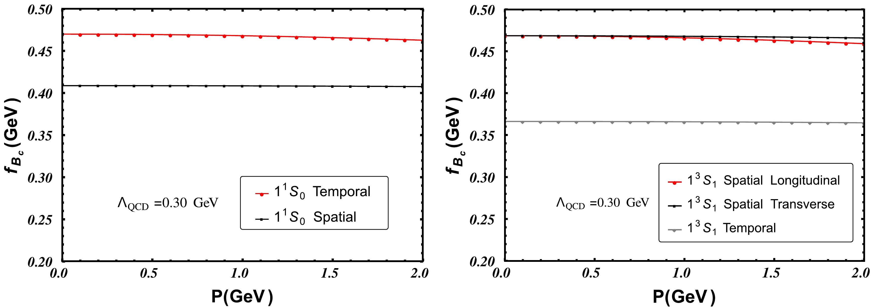

Figure 1

Figure 1.  (color online) Decay constants calculated using Parameter2 in Table 1; the horizontal coordinate is the momentum of the meson. Left: decay constant of $B_c(1^1S_0)$; "$1^1S_0$ Temporal" is calculated from Eq. (12), and "$1^1S_0$ Spatial" is calculated from Eq. (13). Right: decay constant of $B_c(1^3S_1)$; "$1^3S_1$ Temporal" is calculated from Eq. (18), "$1^3S_1$ Spatial Longitudinal" is calculated from Eq. (19), and "$1^3S_1$ Spatial Transverse" is calculated from Eq. (20).

DownLoad: Full-Size Img PowerPoint

Table 4

Table 4.  Our results of decay constants (in GeV) of $B_c(nS)$ and $B^*_c(nS)$ corresponding to the three parameter sets in Table 1; the uncertainties due to losing Lorentz covariance are listed in parentheses.

State	$J^{P}$	$f^{\rm{QM}}_{c\bar{b}}$
		Parameter1	Parameter2	Parameter3
$B_c(1\,^1S_0)$	$0^{-}$	0.429(30)	0.439(30)	0.456(32)
$B_c(2\,^1S_0)$	$0^{-}$	0.292(12)	0.282(13)	0.277(13)
$B_c(3\,^1S_0)$	$0^{-}$	0.251(5)	0.237(6)	0.230(6)
$B^*_c(1\,^3S_1)$	$1^{-}$	0.390(44)	0.417(51)	0.440(56)
$B^*_c(2\,^3S_1)$	$1^{-}$	0.294(33)	0.297(35)	0.296(37)
$B^*_c(3\,^3S_1)$	$1^{-}$	0.262(28)	0.257(29)	0.253(30)

DownLoad: CSV

Show Table

Our final prediction for the decay constant together with both uncertainties are listed in Table 5. We also compare our result with others. $f^{\rm{DSE}}_{c\bar{b}}$ is the result from Dyson-Schwinger equation (DSE) approach [27, 29]. $f^{\rm{lQCD}}_{c\bar{b}}$ is one of the lattice QCD results [44]; the other lattice QCD results are almost consistent with this one. The sixth and seventh columns are results from other potential models [45, 46]. The eighth column is the result from a light-front quark model [47]. These results are almost consistent except that our predictions for the radial excited mesons are smaller than those of Ref. [46]. The main difference is that Ref. [46] uses the nonrelativistic limit van Royen and Weisskopf formula to calculate the decay constants, and this results in a larger decay constant [41]. The reliability of our results can also be supported by the mass spectra and decay constants of the charmonium and bottomium, which are presented in the appendixes. We can see from Table A1, Table A2, Table B1 and Table B2 that our results are overall consistent with other results.

Table 5

Table 5.  Decay constants of $B_c(nS)$ and $B^*_c(nS)$ (in GeV). $f^{\rm{QM}}_{c\bar{b}}$ is our prediction, where the first uncertainty is due to losing Lorentz covariance and the second uncertainty is due to varying the parameters. $f^{\rm{DSE}}_{c\bar{b}}$ are the results from Dyson-Schwinger equation approach, $f_{B_c(1\,^1S_0)}$ and $f_{B^*_c(1\,^3S_1)}$ are from Ref. [29], and $f_{B_c(2\,^1S_0)}$ and $f_{B^*_c(2\,^3S_1)}$ are from Ref. [27]. $f^{\rm{lQCD}}_{c\bar{b}}$ are the lattice QCD results [44]. The sixth and seventh columns are results from other potential models [45, 46]. The eighth column is the result from a light-front quark model [47].

State	$J^{P}$	$f^{\rm{QM}}_{c\bar{b}}$	$f^{\rm{DSE}}_{c\bar{b}}$ [27, 29]	$f^{\rm{lQCD}}_{c\bar{b}}$ [44]	$|f|$ [45]	$|f|$ [46]	$|f|$ [47]
$B_c(1\,^1S_0)$	$0^{-}$	0.439(30)(17)	0.441(1)	0.434(15)	$0.400(45)$	0.433	$0.389^{+16}_{-3}$
$B_c(2\,^1S_0)$	$0^{-}$	0.282(13)(10)	0.246(7)	–	$0.280(50)$	0.356	–
$B_c(3\,^1S_0)$	$0^{-}$	0.237(6)(14)	–	–	–	0.326	–
$B^*_c(1\,^3S_1)$	$1^{-}$	0.417(51)(27)	0.431(7)	0.422(13)	–	0.435	$0.391^{+4}_{-5}$
$B^*_c(2\,^3S_1)$	$1^{-}$	0.297(35)(3)	0.305(13)	–	–	0.356	–
$B^*_c(3\,^3S_1)$	$1^{-}$	0.257(29)(5)	–	–	–	0.326	–

DownLoad: CSV

Show Table

V. SUMMARY AND CONCLUSION

• I. INTRODUCTION
• II. MODEL
• III. DECAY CONSTANT
• IV. RESULTS
• V. SUMMARY AND CONCLUSION
• ACKNOWLEDGEMENTS
• APPENDIX A
• APPENDIX B

In summary, we calculate the decay constants of $B_c(nS)$ and $B^*_c(nS)$ mesons ($n = 1,2,3$) in the nonrelativistic quark model. Our approach can be distinguished from other quark model studies by three points:

(1) The effect of a running strong coupling is taken into account. We use the form Eq. (9), which approaches the one loop running form of QCD at large $Q^2$ and saturates at low $Q^2$. A running coupling affects the wave function of Eq. (1), so it has a considerable effect on the mixing angles and the decay constants.

(2) The ambiguity due to losing Lorentz covariance is discussed in detail. We obtain two different expressions for $f_P$ and three different expressions for $f_V$ in the nonrelativistic quark model as a result of losing Lorentz covariance. The central value is treated as the prediction, and the deviation is treated as the uncertainty. We also find that the uncertainties due to losing Lorentz covariance decrease as n increases.

(3) We use three parameter sets, and the uncertainties due to varying the parameters are given. In most cases, this uncertainty is smaller than the former one.

Comparing our results with those from other approaches, we see that they are in good agreement. While the lattice QCD and DSE approaches meet difficulties dealing with radial excited hadrons, the quark model can be extended to higher excited hadrons easily once the interaction is well constrained. In the appendixes, we compare the decay constants of charmonium and bottomium from our calculation and those from other approaches. The overall agreement also raises the credibility of our approach. Overall, the decay constants of $B_c(nS)$ and $B^*_c(nS)$ mesons ($n = 1,2,3$) are predicted, with the uncertainties well determined. We thus establish a good basis to study the decays of $B_c$ mesons.

ACKNOWLEDGEMENTS

• I. INTRODUCTION
• II. MODEL
• III. DECAY CONSTANT
• IV. RESULTS
• V. SUMMARY AND CONCLUSION
• ACKNOWLEDGEMENTS
• APPENDIX A
• APPENDIX B

We thank Professor Xianhui Zhong for careful reading of the manuscript and for his useful suggestions.

APPENDIX A

• I. INTRODUCTION
• II. MODEL
• III. DECAY CONSTANT
• IV. RESULTS
• V. SUMMARY AND CONCLUSION
• ACKNOWLEDGEMENTS
• APPENDIX A
• APPENDIX B

In this appendix, we list our nonrelativistic quark model results of the mass spectrum of charmonium in Table A1 and the decay constants of $\eta_c(nS)$ and $J/\psi(nS)$ (n = 1, 2, 3) in Table A2. The experimental values of the vector meson decay constants ($f_V$) in Table A2 and Table B2 are estimated by

where $\Gamma_{V\to e^+e^-}$ is the decay width of the vector meson to $e^+e^-$, α is the fine structure constant, Q is the electric charge of the constituent quark, and $M_V$ is the mass of the vector meson.

Table A1

Table A1.  Mass spectrum of charmonium (in GeV). $M_{c\bar{c}}^{\text{QM}}$ is our nonrelativistic quark model result, with the parameters $m_c = 1.591 \text{ GeV}$, $\alpha_0 = 1.082$, $N_f = 4$, $\Lambda_{\text{QCD}} = 0.30 \text{ GeV}$, $b = 0.1320 \text{ GeV}^2$, $\sigma = 1.30 \text{ GeV}$, $r_c = 0.375 \text{ fm}$. Note that $N_f$ and $\Lambda_{\text{QCD}}$ are chosen according to QCD estimatation, the other parameters are tuned to fit the masses of $\eta_c(1S)$, $\eta_c(2S)$, $J/\psi(1S)$ and $\chi_{c0}(1P)$, i.e. these four masses are inputs of our model, and all the other masses are outputs. $M^{\rm{expt.}}_{c\bar{c}}$ are the experiment values [42].

$n^{2S+1}L_J$	State	$J^{PC}$	$M_{c\bar{c}}^{\text{QM}}$	$M^{\rm{expt.}}_{c\bar{c}}$ [42]
$1^1S_0$	$\eta_c(1S)$	$0^{-+}$	2.984 (input)	2.984(0.4)
$2^1S_0$	$\eta_c(2S)$	$0^{-+}$	3.639 (input)	3.638(1)
$3^1S_0$	$\eta_c(3S)$	$0^{-+}$	4.054	–
$1^3S_1$	$J/\psi(1S)$	$1^{--}$	3.097 (input)	3.097(0)
$2^3S_1$	$\psi(2S)$	$1^{--}$	3.687	3.686(0.1)
$3^3S_1$	$\psi(4040)$	$1^{--}$	4.088	4.039(1)
$1^3P_0$	$\chi_{c0}(1P)$	$0^{++}$	3.415 (input)	3.415(0.3)
$2^3P_0$	$\chi_{c0}(2P)$	$0^{++}$	3.897	–
$3^3P_0$	$\chi_{c0}(3P)$	$0^{++}$	4.260	–
$1^1P_1$	$h_{c}(1P)$	$1^{+-}$	3.498	3.525(0.1)
$2^1P_1$	$h_{c}(2P)$	$1^{+-}$	3.931	–
$3^1P_1$	$h_{c}(3P)$	$1^{+-}$	4.279	–
$1^3P_1$	$\chi_{c1}(1P)$	$1^{++}$	3.492	3.511(0.1)
$2^3P_1$	$\chi_{c1}(2P)$	$1^{++}$	3.934	–
$3^3P_1$	$\chi_{c1}(3P)$	$1^{++}$	4.285	–
$1^3P_2$	$\chi_{c2}(1P)$	$2^{++}$	3.534	3.556(0.1)
$2^3P_2$	$\chi_{c2}(3930)$	$2^{++}$	3.956	3.923(1)
$3^3P_2$	$\chi_{c2}(3P)$	$2^{++}$	4.299	–

DownLoad: CSV

Show Table

Table A2

Table A2.  Decay constants of $\eta_c(nS)$ and $J/\psi(nS)$ (in GeV). $f^{\rm{QM}}_{c\bar{c}}$ are our nonrelativistic quark model results, with the parameters listed in the caption of Table A1. The uncertainties due to losing Lorentz covariance are listed in parentheses. $f^{\rm{DSE}}_{c\bar{c}}$ are the results from Dyson-Schwinger equation (DSE) approach, where $f_{\eta_c(1\,^1S_0)}$ and $f_{J/\psi(1\,^3S_1)}$ are from Ref. [29], $f_{\eta_c(2\,^1S_0)}$ and $f_{\psi(2\,^3S_1)}$ are from Ref. [27], and the underlined values are inputs. $f^{\rm{lQCD}}_{c\bar{b}}$ are the lattice QCD results, where $f_{\eta_c(1\,^1S_0)}$ is from Ref. [48], and $f_{J/\psi(1\,^3S_1)}$ is from Ref. [49]. The seventh and eighth columns are other potential model results [45, 46]. The ninth column is a light front quark model result [47]. $f^{\rm{SR}}_{c\bar{c}}$ are the results from QCD sum rule [50]. $f^{\rm{expt.}}_{c\bar{c}}$ are the experimental values and the vector meson decay constant is estimated by Eq. (25).

$n^{2S+1}L_J$	State	$J^{PC}$	$f^{\rm{QM}}_{c\bar{c}}$	$f^{\rm{DSE}}_{c\bar{c}}$ [27, 29]	$f^{\rm{lQCD}}_{c\bar{c}}$ [48,49]	$|f|$ [45]	$|f|$ [46]	$|f|$ [47]	$f^{\rm{SR}}_{c\bar{c}}$ [50]	$f^{\rm{expt.}}_{c\bar{c}}$ [42]
$1\,^1S_0$	$\eta_c(1S)$	$0^{-+}$	0.447(32)	0.393	0.393(4)	–	0.350	$0.353^{+22}_{-17}$	0.309(39)
$2\,^1S_0$	$\eta_c(2S)$	$0^{-+}$	0.268(2)	0.223(11)	–	–	0.278	–	–
$3\,^1S_0$	$\eta_c(3S)$	$0^{-+}$	0.220(11)	–	–	–	0.249	–	–
$1\,^3S_1$	$J/\psi$	$1^{--}$	0.403(57)	0.430(1)	0.405(6)	0.400(35)	0.326	$0.361^{+7}_{-6}$	0.401(46)	0.416(8)
$2\,^3S_1$	$\psi(2S)$	$1^{--}$	0.295(35)	0.294(7)	–	0.297(26)	0.257	–	–	0.294(5)
$3\,^3S_1$	$\psi(3S)$	$1^{--}$	0.257(26)	–	–	0.226(20)	0.230	–	–	0.187(15)

DownLoad: CSV

Show Table

APPENDIX B

• I. INTRODUCTION
• II. MODEL
• III. DECAY CONSTANT
• IV. RESULTS
• V. SUMMARY AND CONCLUSION
• ACKNOWLEDGEMENTS
• APPENDIX A
• APPENDIX B

In this appendix, we list our nonrelativistic quark model results of the mass spectrum of charmonium in Table B1 and the decay constants of $\eta_b(nS)$ and $\varUpsilon(nS)$ (n=1, 2, 3) in Table B2.

Table B1

Table B1.  Mass spectra of bottomium (in GeV). $M_{b\bar{b}}^{\text{QM}}$ are our nonrelativistic quark model results, with the parameters $m_b = 4.997\ \text{ GeV}$, $\alpha_0 = 0.920$, $N_f = 5$, $\Lambda_{\text{QCD}} = 0.30\ \text{ GeV}$, $b = 0.1110\ \text{ GeV}^2$, $\sigma = 2.35\ \text{ GeV}$, $r_c = 0.195\ \text{ fm}$. Note that $N_f$ and $\Lambda_{\text{QCD}}$ are chosen by QCD estimatation, the other parameters are tuned to fit the masses of $\eta_b(1S)$, $\varUpsilon(1S)$, $\varUpsilon(2S)$ and $\chi_{b0}(1P)$, i.e. these four masses are inputs of our model, and all the other masses are outputs. $M^{\rm{expt.}}_{b\bar{b}}$ are the experimental values [42].

$n^{2S+1}L_J$	State	$J^{{PC} }$	$M^{\text{QM}}_{b\bar{b}}$	$M^{\text{expt.}}_{b\bar{b}}$ [42]
$1^1S_0$	$\eta_b(1S)$	$0^{-+}$	9.400 (input)	9.399(2)
$2^1S_0$	$\eta_b(2S)$	$0^{-+}$	10.004	9.999(4)
$3^1S_0$	$\eta_b(3S)$	$0^{-+}$	10.324	–
$1^3S_1$	$\varUpsilon(1S)$	$1^{--}$	9.460 (input)	9.460(0.3)
$2^3S_1$	$\varUpsilon(2S)$	$1^{--}$	10.023 (input)	10.023(0.3)
$3^3S_1$	$\varUpsilon(3S)$	$1^{--}$	10.336	10.355(1)
$4^3S_1$	$\varUpsilon(4S)$	$1^{--}$	10.573	10.579(1)
$1^3P_0$	$\chi_{b0}(1P)$	$0^{++}$	9.859 (input)	9.859(1)
$2^3P_0$	$\chi_{b0}(2P)$	$0^{++}$	10.224	10.233(1)
$3^3P_0$	$\chi_{b0}(3P)$	$0^{++}$	10.481	–
$1^1P_1$	$h_{b}(1P)$	$1^{+-}$	9.903	9.899(1)
$2^1P_1$	$h_{b}(2P)$	$1^{+-}$	10.244	10.260(1)
$3^1P_1$	$h_{b}(3P)$	$1^{+-}$	10.493	–
$1^3P_1$	$\chi_{b1}(1P)$	$1^{++}$	9.896	9.893(1)
$2^3P_1$	$\chi_{b1}(2P)$	$1^{++}$	10.242	10.255(1)
$3^3P_1$	$\chi_{b1}(3P)$	$1^{++}$	10.493	10.513(1)
$1^3P_2$	$\chi_{b2}(1P)$	$2^{++}$	9.921	9.912(1)
$2^3P_2$	$\chi_{b2}(2P)$	$2^{++}$	10.255	10.269(1)
$3^3P_2$	$\chi_{b2}(3P)$	$2^{++}$	10.502	10.524(1)
$1^3D_2$	$\varUpsilon_2(1D)$	$2^{--}$	10.152	10.164(1)

DownLoad: CSV

Show Table

Table B2

Table B2.  Decay constants of $\eta_b(nS)$ and $\varUpsilon(nS)$ (in GeV). $f^{\rm{QM}}_{b\bar{b}}$ are our nonrelativistic quark model results, with the parameters listed in the caption of Table B1. The uncertainties due to losing Lorentz covariance are listed in parentheses. $f^{\rm{DSE}}_{b\bar{b}}$ are the results from the Dyson-Schwinger equation (DSE) approach, where $f_{\eta_b(1\,^1S_0)}$ and $f_{\varUpsilon(1\,^3S_1)}$ are from Ref. [29], $f_{\eta_b(2\,^1S_0)}$ and $f_{\varUpsilon(2\,^3S_1)}$ are from Ref. [27], and the underlined values are inputs. $f^{\rm{lQCD}}_{c\bar{b}}$ are the lattice QCD results, where $f_{\eta_b(1\,^1S_0)}$ are from Ref. [48], and $f_{\varUpsilon(1\,^3S_1)}$ and $f_{\varUpsilon(2\,^3S_1)}$ are from Ref. [51]. The seventh and eighth columns are other potential model results [45, 46]. The ninth column is a light front quark model result [47]. $f^{\rm{expt.}}_{b\bar{b}}$ are the experimental values and the vector meson decay constant is estimated by Eq. (25).

$n^{2S+1}L_J$	State	$J^{\rm{PC}}$	$f^{\rm{QM}}_{b\bar{b}}$	$f^{\rm{DSE}}_{b\bar{b}}$ [27,29]	$f^{\rm{lQCD}}_{b\bar{b}}$ [48,51]	$|f|$ [45]	$|f|$ [46]	$|f|$ [47]	$f^{\rm{expt.}}_{b\bar{b}}$ [42]
$1\,^1S_0$	$\eta_b(1S)$	$0^{-+}$	0.749(41)	0.667	0.667(6)	–	0.646	$0.605^{+32}_{-17}$
$2\,^1S_0$	$\eta_b(2S)$	$0^{-+}$	0.441(14)	0.488(8)	–	–	0.519	–
$3\,^1S_0$	$\eta_b(3S)$	$0^{-+}$	0.356(7)	–	–	–	0.475	–
$1\,^3S_1$	$\varUpsilon(1S)$	$1^{--}$	0.712(78)	0.625(4)	0.649(31)	0.685(30)	0.647	$0.611^{+6}_{-11}$	0.715(10)
$2\,^3S_1$	$\varUpsilon(2S)$	$1^{--}$	0.460(48)	0.498(6)	0.481(39)	0.469(21)	0.519	–	0.497(9)
$3\,^3S_1$	$\varUpsilon(3S)$	$1^{--}$	0.381(38)	–	–	0.399(17)	0.475	–	0.425(8)

DownLoad: CSV

Show Table

References