


 Abstract
 HTML
HTML Reference
 Related
 PDF
PDF


-
The electromagnetic form factors of nucleons are important physical quantities, which are helpful to understand both the nucleon inner structure and the mechanism of strong interaction. For many years, the elastic lepton-nucleon scattering measurements have enabled us to obtain detailed information on the electromagnetic form factors of the proton and neutron over a wide range of kinematics. Numerous measurements were carried out at the Stanford Mark III accelerator [1], Cambridge Electron Accelerator [2], Stanford Linear Accelerator Center (SLAC) [3], Bonn [4], DESY [5], Mainz [6], NIKHEF [7], MIT-Bates [8], and Jefferson Lab [9]. The elastic scattering measurements have stimulated considerable activity over the past two decades in the determination of the flavor separated form factors of the up, down, and strange quarks in the nucleon. A number of measurements of the strange form factors have been successfully performed, starting with SAMPLE at Bates [10] and A4 at Mainz [11], followed by the high precision G0 [12] and HAPPEX [13] experiments at Jefferson Lab.
Numerous theoretical works have also been perfomed on the nucleon form factors. Owing to the non-perturbative property of the strong interaction, it is very difficult to study hadron properties using the QCD fundamental theory directly. Many theoretical calculations are based on phenomenological methods, such as the constituent quark model, cloudy bag model, perturbative chiral quark model, quark-diquark model, nonlocal quark meson coupling model, Nambu-Jona-Lasinio model, Dyson-Schwinger equations, vector meson dominance model, chiral quark soliton model, and AdS/QCD approach [14–30]. The lattice QCD simulation is the most rigorous method to study hadron properties. However, the simulated results have to be extrapolated to the continuum and infinite volume limits to compare them with experimental data. In addition, if the simulations are performed using heavy quark masses, the data need to be extrapolated to the physical quark masses. With the improvement in computing speed, currently, lattice simulation of nucleon form factors can be carried out at physical quark masses including the disconnected contributions [31, 32].
Besides lattice QCD, the chiral effective field theory (EFT) is another systematic approach that has been widely applied in hadron physics [33, 34]. Compared with the various phenomenological models, one advantage of the EFT is that it can provide some model-independent results. Although the chiral EFT has been a fairly successful approach, for the nucleon form factors it is only valid at relatively small
$ Q^2 $ values, for example, less than 0.1 GeV$ ^2 $ [35]. The range can be extended up to 0.4 GeV$ ^2 $ by explicitly including vector meson degrees of freedom into the theory [36].In recent years, we proposed a nonlocal chiral effective theory, which makes it possible to study hadron properties at a relatively large momentum transfer [37]. The basic idea is that in the nonlocal Lagrangian, a baryon and a meson are located in different coordinates described by a correlator. To guarantee the local gauge invariance, the path integral of the gauge field is introduced, which leads to the additional interactions. The additional Feynman diagrams are crucial to obtain the corrected normalized nucleon charge. On the one hand, the correlator makes the loop integral ultraviolet convergent. On the other hand, the physical quantities at a large momentum transfer can be described very well. Perturbative calculations in chiral EFT expand the observables as series in the pseudoscalar meson mass
$ {\cal O}(m_\phi/\Lambda_{\chi}) $ or small external momentum$ {\cal O}(q/\Lambda_{\chi}) $ , where$ \Lambda_{\chi} \sim 1 $ GeV is the scale associated with the chiral EFT. With the introducing of the regulator, the power counting of our nonlocal EFT is lost. The higher order terms are included as a type of resummation. This resummation of the chiral expansion induced through the introduction of a finite range cutoff in the momentum integrals of meson-loop diagrams has been shown to be a very good and effective resummation method. The nonlocal chiral EFT has been applied to study the nucleon electromagnetic form factors [38], strange form factors [39], unpolarized and polarized parton distribution functions (PDFs) [40–42], generalized parton distributions (GPDs) [43], etc. The approach has also been generalized to the fundamental interaction of QED, which provided an interesting explanation to the lepton$ g-2 $ anomaly [44, 45].In the previous form factor calculations, the bubble and tadpole diagrams were not included [38, 39, 46]. In fact, in the earlier extrapolation of nucleon form factors with finite-range regularization, these diagrams were not included either [47, 48]. The bubble and tadpole diagrams have no effect on the nucleon wave function renormalization because their contributions to the nucleon charge are summed to be zero. In this work, we will apply the nonlocal EFT to study the nucleon form factors, including these bubble and tadpole diagrams, to verify whether the results are changed or not. This paper is organized in the following way. In Sec. II, we briefly introduce the nonlocal chiral effective Lagrangian. The matrix elements of the bubble and tadpole diagrams for the electromagnetic and strange form factors are presented in Sec. III. Numerical results are discussed in Sec. IV. Finally, Sec. V is a brief summary.
-
We start from the local chiral effective Lagrangian. The lowest Lagrangian that describes the pseudoscalar mesons, octet and decuplet baryons, and their interaction is expressed as
$ \begin{aligned}[b] \mathcal{L}^{(1)} = & {\rm Tr}\big[\bar{B}\left({\rm i}\not {\mathcal{D}}-M_{B}\right)B\big]+D\,{\rm Tr}\left[\bar{B}\gamma^{\mu}\gamma^{5}\left\{ u_{\mu},B\right\} \right]\\ &+F\,{\rm Tr}\left[\bar{B}\gamma^{\mu}\gamma_{5}\left[u_{\mu},B\right]\right] +\overline{T}_{\mu}^{ijk}\left({\rm i}\gamma^{\mu\nu\alpha}\mathcal{D}_{\alpha}+{\rm i}M_{T}\sigma^{\mu\nu}\right)T_{\nu}^{ijk}\\ & +\mathcal{C}\left[\epsilon^{ijk}\overline{T}_{\mu}^{ ilm}\Theta^{\mu\nu}\left(u_{\nu}\right)^{lj}B^{mk}+\text{h.c.}\right] \\ & +\mathcal{H}\,\overline{T}_{\mu}^{ ijk}\gamma^{\mu\nu\alpha}\gamma^{5}\left(u_{\alpha}\right)^{kl}T_{\nu}^{ijl}+\frac{f^{2}}{4}{\rm Tr}\big[\partial_{\mu}U\left(\partial^{\mu}U\right)^{\dagger}\big],\\[-15pt] \end{aligned} $

(1) where D, F,
$ {\cal C} $ , and$ \mathcal{H} $ are the baryon-meson coupling constants.$ M_{B} $ and$ M_{T} $ are the octet and decuplet baryon masses.$ f\thickapprox93 $ MeV is the pseudoscalar decay constant. The$ \Theta^{\mu\nu} $ in the octet-decuplet transition operator is given by$ \begin{array}{*{20}{l}} \Theta^{\mu\nu}=g^{\mu\nu}-Z\gamma^{\mu}\gamma^{\nu}, \end{array} $

(2) where Z is the off shell parameter. The tensor
$ \gamma^{\mu\nu\alpha} $ is defined as$\gamma^{\mu\nu\alpha}=-{\rm i}\left\{ \sigma^{\mu\nu},\gamma^{\alpha}\right\}$ . The octet baryons and mesons are arranged in$ 3\times 3 $ matrices, while the decuplet baryons are represented by the symmetric tensor with three indices. The covariant derivatives of the octet and decuplet baryon fields are given by$ \mathcal{D}_{\mu}B=\partial_{\mu}B+[\Gamma_{\mu},B], \quad \mathcal{D_{\mu}}T_{\nu}^{ijk}=\partial_{\mu}T_{\nu}^{ijk}+(\Gamma_{\mu},T_{\nu})^{ijk}.$

(3) The mesons couple to the baryon fields through the vector and axial vector combinations defined as
$ \begin{aligned}[b] & \Gamma_{\mu}=\frac{1}{2}(u\partial_{\mu}u^{\dagger}+u^{\dagger}\partial_{\mu}u), ~~ u_{\mu}=\frac{{\rm i}}{2}(u\partial_{\mu}u^{\dagger}-u^{\dagger}\partial_{\mu}u), \end{aligned} $

(4) where
$ {u} $ is defined in terms of the pseudoscalar meson field$ {\phi} $ $ u^{2}=\exp\left({\rm i}\frac{\sqrt{2}\phi}{f}\right). $

(5) The octet, decuplet, and octet-decuplet transition magnetic moment operators are needed in the one loop calculation of nucleon form factors. The magnetic Lagrangian is written as
$ \begin{aligned}[b] {\cal L}_{\text{mag}} =&\frac{e}{4M_{B}}(c_{1} {\rm{Tr}}[\overline{B}\sigma^{\mu\nu}\{\mathcal{F}_{\mu\nu}^{\dagger},B\}]+c_{2} {\rm{Tr}}[\overline{B}\sigma^{\mu\nu}[\mathcal{F}_{\mu\nu}^{\dagger},B]]\\&+c_{3} {\rm{Tr}}[\mathcal{F}_{\mu\nu}^{\dagger}] {\rm{Tr}}[\overline{B}\sigma^{\mu\nu}B]) -\frac{eF_{2}^{T}}{4M_{T}}\overline{T}_{\mu}^{abc}\sigma^{\alpha\beta}\mathcal{F}_{\alpha\beta}Q^{ce}T^{\mu,eba} \\ & +\frac{{\rm i}ec_{4}}{4M_{B}}\mathcal{F}_{\mu\nu}(\epsilon^{ ijk}\overline{B}^{jm}Q^{il}\gamma^{\mu}\gamma^{5}T^{\nu,klm}\\&+\epsilon^{ ijk}\overline{T}^{\mu,klm}Q^{li}\gamma^{\nu}\gamma^{5}B^{mj}),\\[-10pt] \end{aligned} $

(6) where
$ c_{1} $ ,$ c_{2} $ , and$ c_{3} $ describe the magnetic moments of octet baryons at tree levels, whereas$ F_2^T $ and$ c_4 $ are related to the magnetic moments of the decuplet baryons and octet-decuplet transition. With the$ S U(6) $ symmetry, one can have the following relationships [43]:$ \begin{aligned}[b] c_3 =& c_2 - c_1, \\ F_{2}^T =&\frac{1}{3}(c_{1}+3c_{2}),\\ c_4 =& \frac{1}{\sqrt{3}}c_{1}. \end{aligned} $

(7) To calculate the contributions of the bubble diagrams, the following high order Lagrangian that provides the next-to-leading order baryon-baryon-meson-meson interaction has to be included [49]:
$ \begin{aligned}[b] \mathcal{L}^{(2)}=&\frac{\rm i}{2}\sigma^{\mu\nu}(b_{9} {\rm{Tr}}[\overline{B}u_{\mu}] {\rm{Tr}}[u_{\nu}B]+b_{10} {\rm{Tr}}[\overline{B}\{[u_{\mu},u_{\nu}],B\}]\\&+b_{11} {\rm{Tr}}[\overline{B}[[u_{\mu},u_{\nu}],B]]), \end{aligned} $

(8) where the coefficients
$ b_{9} $ ,$ b_{10} $ , and$ b_{11} $ are determined in Ref. [49] as$ b_{9}=1.36 $ GeV,$ b_{10}=1.24 $ GeV, and$b_{11} = 0.46$ GeV.The gauge invariant nonlocal Lagrangian can be obtained by the displacement of the coordinates of the meson and photon fields with the proper inclusion of the gauge link. For example, the gauge invariant local strong interaction
$ pp\pi\pi $ is expressed as$ \begin{aligned}[b] {\cal L}_{\pi\pi}^{\text{local}}=&\frac{\rm i}{4f^{2}}\overline{p}(x)\gamma^{\mu}p(x)\Big[\pi^+(x)(\partial_\mu -{\rm i}eA_\mu(x))\pi^-(x)\\&-\pi^-(x)(\partial_\mu+{\rm i}eA_\mu(x))\pi^+(x)\Big]. \end{aligned} $

(9) The corresponding nonlocal Lagrangian is expressed as
$ \begin{aligned}[b]\\[-8pt] {\cal L}_{\pi\pi}^{\text{nl}} = & \frac{{\rm i}}{4f^{2}}\overline{p}(x)\gamma^{\mu}p(x)\int {\rm d}a\int {\rm d}bF(a)F(b) \Big[\text{exp}\Big[{\rm i}e\int_{x}^{x+a}{\rm d}z_{\nu}\int {\rm d}c\mathcal{A}^{\nu}(z-c)F(c)\Big]\pi^+(x+a) \\ & \times (\partial_{\mu}-{\rm i}e\int {\rm d}cF(c)\mathcal{A}_{\mu}(x-c))\text{exp}\Big[-{\rm i}e\int_{x}^{x+b}{\rm d}z_{\nu}\int {\rm d}c\mathcal{A}^{\nu}(z-c)F(c)\Big]\pi^-(x+b)\\ & - (\partial_{\mu}+{\rm i}e\int {\rm d}cF(c)\mathcal{A}_{\mu}(x-c))\text{exp}\Big[{\rm i}e\int_{x}^{x+a}{\rm d}z_{\nu}\int {\rm d}c\mathcal{A}^{\nu}(z-c)F(c)\Big]\pi^+(x+a) \\ & \times \text{exp}\Big[-{\rm i}e\int_{x}^{x+b}{\rm d}z_{\nu}\int {\rm d}c\mathcal{A}^{\nu}(z-c)F(c)\Big]\pi^-(x+b)\Big], \end{aligned} $ 
(10) where
$ F(a) $ is the correlation function. To guarantee the gauge invariance, the gauge links are introduced in the above Lagrangian. Similarly, the nonlocal electromagnetic interaction of the nucleon can also be obtained. For example, the local interaction between a proton and a photon is written as$ \begin{align} {\cal L}_{\text{EM}}^{\text{local}}= & -e\bar{p}(x)\gamma^{\mu}p(x)\mathcal{A}_{\mu}(x)+\frac{(c_{1}+3c_{2})e}{12m_{N}}\bar{p}(x)\sigma^{\mu\nu}p(x)F_{\mu\nu}(x). \end{align} $

(11) The corresponding nonlocal Lagrangian is expressed as
$ \begin{aligned}[b] {\cal L}_{\text{EM}}^{\text{nl}}=&-e\int {\rm d}a\bar{p}(x)\gamma^{\mu}p(x)\mathcal{A}_{\mu}(x-a)F_{1}(a)\\&+\frac{(c_{1}+3c_{2})e}{12m_{N}}\int {\rm d}a\bar{p}(x)\sigma^{\mu\nu}p(x)F_{\mu\nu}(x-a)F_{2}(a), \end{aligned} $

(12) where
$ F_{1}(a) $ and$ F_{2}(a) $ are the correlation functions for the nonlocal electric and magnetic interactions. As in our previous work, we assume that the charge and magnetic form factors at the tree level have the same momentum dependence as the nucleon-pion vertex, i.e.,$ G_{M}^{{\rm tree}}(p)= \mu_p G_{E}^{{\rm tree}}(p)= \mu_p \tilde{F}(p) $ , where$ \tilde{F}(p) $ is the Fourier transformation of the correlation function$ F(a) $ . Therefore, the corresponding functions of$ \tilde{F}_{1}(q) $ and$ \tilde{F}_{2}(q) $ are expressed as$ \begin{aligned}[b] \tilde{F}_{1}(q) = \tilde{F}(q)\frac{4m_{N}^{2}+\mu_{p}Q^{2}}{4m_{N}^{2}+Q^{2}},\; \; \; \tilde{F}_{2}(q)=\tilde{F}(q)\frac{(\mu_{p}-1)4m_{N}^{2}}{4m_{N}^{2}+Q^{2}}. \end{aligned} $

(13) The nonlocal Lagrangian is invariant under the following gauge transformation
$ \begin{aligned}[b] &\pi^+(y)\rightarrow {\rm e}^{{\rm i}\alpha(y)}\pi^+(y),\; \; \; \; p(x)\rightarrow {\rm e}^{{\rm i}\alpha(x)}p(x),\; \; \; \;\\& \mathcal{A}_{\mu}(x)\rightarrow \,\mathcal{A}_{\mu}(x)-\frac{1}{e}\partial_{\mu}\alpha'(x), \end{aligned} $

(14) where
$\alpha(x)=\int \,{\rm d}a\alpha^{\prime}(x-a)F(a)$ .From the nonlocal Lagrangian, the interaction with the external photon can be obtained. There are two types of electromagnetic interactions in a nonlocal case. Besides that from the minimal substitution, which is the same as in the local interaction, there is an additional one generated from the expansion of the gauge link. For example, from Eq. (10), we can obtain the additional interaction as
$ \begin{aligned}[b] {\cal L}^{\text{add}} =&-\frac{e}{4f^{2}}\overline{p}(x)\gamma^{\mu}p(x)\int {\rm d}a\int {\rm d}bF(a) F(b)\\&\times\Big[\int_{x}^{x+a}{\rm d}z_{\nu}\int {\rm d}c\mathcal{A}^{\nu}(z-c)F(c)\pi^+(x+a)\partial_{\mu}\pi^-(x+b) \\ & -\pi^+(x+a)\partial_{\mu}\Big(\int_{x}^{x+b}{\rm d}z_{\nu}\int {\rm d}c\mathcal{A}^{\nu}(z-c)F(c)\pi^-(x+b)\Big) \\ & -\partial_{\mu}\Big(\int_{x}^{x+a}{\rm d}z_{\nu}\int {\rm d}c\mathcal{A}^{\nu}(z-c)F(c)\pi^+(x+a)\Big)\pi^-(x+b) \\ & +\partial_{\mu}\pi^+(x+a)\int_{x}^{x+b}{\rm d}z_{\nu}\int {\rm d}c\mathcal{A}^{\nu}(z-c)F(c)\pi^-(x+b)\Big]. \end{aligned} $

(15) The additional interaction is important to acquire the renormalized proton (neutron) charge 1 (0). With the nonlocal Lagrangian, one can calculate the electromagnetic and strange form factors of the nucleon.
-
The Dirac and Pauli form factors of the nucleon are defined as
$ \begin{aligned}[b]& <N(p')|J^{\mu}|N(p)>\\=&\bar{u}(p')\left\{ \gamma^{\mu}F_{1}^{N}(Q^{2})+\frac{{\rm i} \sigma^{\mu\nu}q_{\nu}}{2m_{N}}F_{2}^{N}(Q^{2})\right\} u(p), \end{aligned} $

(16) where
$ q=p^{\prime}-p $ and$ Q^{2}=-q^{2} $ .$ F_{1}^{N}(Q^{2}) $ and$ F_{2}^{N}(Q^{2}) $ are the Dirac and Pauli form factors, respectively. The combination of the above form factors can generate the electric and magnetic form factors as$ \begin{aligned}[b] G_{E}^{N}(Q^{2})=&F_{1}^{N}(Q^{2})-\frac{Q^{2}}{{4m_{N}^{2}}}F_{2}^{N}(Q^{2})\\ G_{M}^{N}(Q^{2})=&F_{1}^{N}(Q^{2})+F_{2}^{N}(Q^{2}). \end{aligned} $

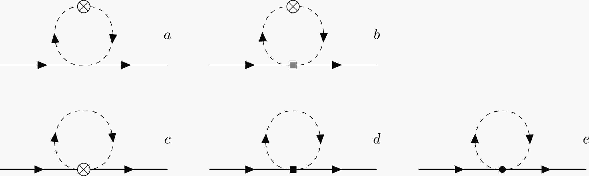
(17) In Eq. (16), the contributions of the u, d, and s quarks are all included in the current. If only the strange current is included, one can obtain the strange form factors. According to the Lagrangian, the one-loop Feynman diagrams that contribute to the nucleon electromagnetic form factors are plotted in Fig. 1, where only bubble and tadpole diagrams are shown. In Fig. 1, diagrams a and b are called bubble diagrams, while c, d, and e are called tadpole diagrams. Here, we only present the formulas for the bubble and tadpole diagrams. The formulas for the other diagrams can be found in Refs. [38, 46].
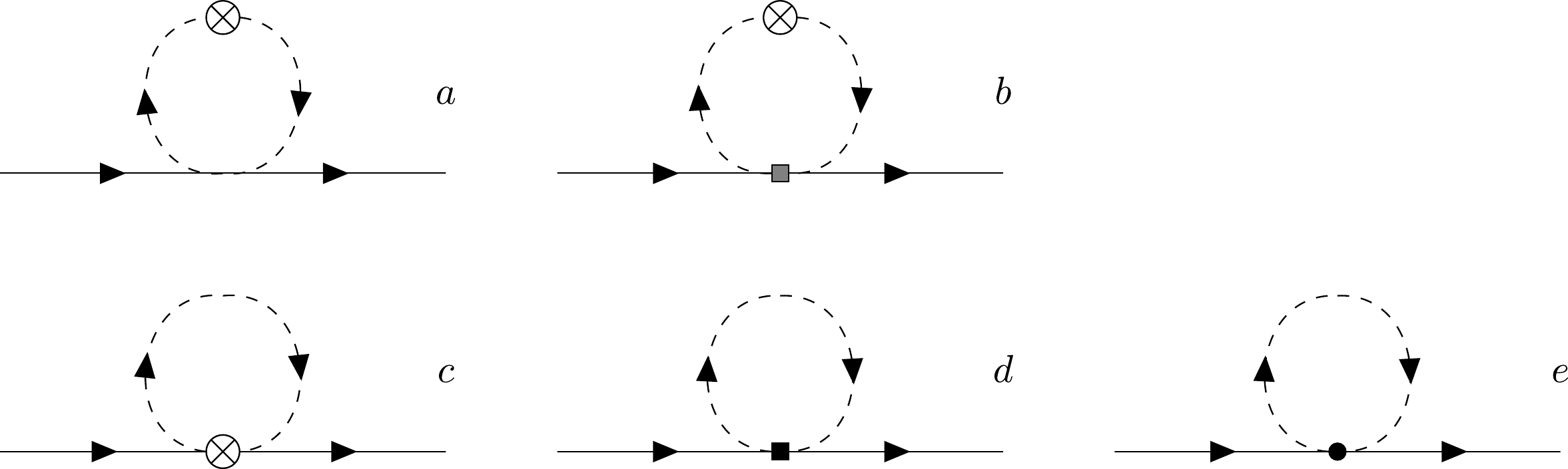
Figure 1. One-loop Feynman diagrams for the nucleon electromagnetic form factors. The solid and dashed lines are for a nucleon and meson, respectively. The crossed circle represents the interaction with the photon field from the minimal substitution, the black square represents the magnetic interaction in Eq. (6), the gray square denotes the interaction in Eq. (8), and the filled circle denotes the additional gauge link interaction with the photon field.
The contributions of the leading bubble diagram, Fig. 1(a), to the matrix elements in Eq. (16) are written as
$ \begin{aligned}[b] \Gamma_{a}^{\mu(p)} & =-\frac{1}{4f^{2}}I^\mu_{a,\pi^+\pi^-}-\frac{1}{2f^{2}}I^\mu_{a,K^+K^-}, \\ \Gamma_{a}^{\mu(n)} & =\frac{1}{4f^{2}}I^\mu_{a,\pi^+\pi^-}-\frac{1}{4f^{2}}I^\mu_{a,K^+K^-}, \\ \Gamma_{a}^{\mu(s)} & =\frac{1}{4f^{2}}I_{a,K^+K^-}^{\mu}+\frac{1}{2f^{2}}I_{a,K^{0}\bar{K}^0}^{\mu}, \end{aligned} $

(18) where the integral
$ I_{a,\phi^+\phi^-}^{\mu} $ is expressed as$ \begin{aligned}[b] I^\mu_{a,\phi^+\phi^-}=&\tilde{F}(q)\,\bar{u}(p')\int \frac{{\rm d}^{4}k}{(2\pi)^{4}}\tilde{F}(k)\frac{1}{D_\phi(k)}\\&\times(2{\not k}+{\not q})2k^{\mu}\tilde{F}(k+q)\frac{1}{D_\phi(k+q)}u(p). \end{aligned} $

(19) Besides the matrix elements for the proton and neutron, the matrix element of the strange quark
$ \Gamma_{a}^{\mu(s)} $ is also written. In the above integral,$ D_\phi(k) $ is the propagator of meson ϕ. The correlators$ \tilde{F}(k) $ and$ \tilde{F}(k+q) $ make the loop integral convergent and$ \tilde{F}(q) $ gives a proper meson form factor at the tree level. The contributions of the bubble diagram at next-to-leading order, Fig. 1(b), to the matrix elements are written as$ \begin{aligned}[b] \Gamma_{b}^{\mu(p)} & =-\frac{2(b_{10}+b_{11})}{f^{2}}I^\mu_{b,\pi^+\pi^-}-\frac{4b_{11}+b_{9}}{f^{2}}I^\mu_{b,K^+K^-}, \\ \Gamma_{b}^{\mu(n)} & =\frac{2(b_{10}+b_{11})}{f^{2}}I^\mu_{b,\pi^+\pi^-}-\frac{2(b_{10}-b_{11})}{f^{2}}I^\mu_{b,K^+K^-},\\ \Gamma_{b}^{\mu(s)} & =-\frac{2(b_{10}-b_{11})}{f^{2}}I_{b,K^+K^-}^{\mu}+\frac{4b_{11}+b_{9}}{f^{2}}I_{b,K^{0}\bar{K}^0}^{\mu}, \end{aligned} $

(20) where the integral
$ I_{b,\phi^+\phi^-}^{\mu} $ is expressed as$ \begin{aligned}[b] I^\mu_{b,\phi^+\phi^-}=&\tilde{F}(q)\,\bar{u}(p')\int \frac{{\rm d}^{4}k}{(2\pi)^{4}}\sigma^{\rho\nu}q_{\rho}k_{\nu}\tilde{F}(k)\frac{1}{D_\phi(k)}\\&\times 2k^{\mu}\tilde{F}(k+q)\frac{1}{D_\phi(k+q)}u(p). \end{aligned} $

(21) For the tadpole diagram with electric coupling to the photon field, Fig. 1(c), the matrix elements are written as
$ \begin{aligned}[b] \Gamma_{c}^{\mu(p)} =&-\frac{4m_{N}^{2}+Q^{2}(1+c_{1}+c_{2})}{2(4m_{N}^{2}+Q^{2})f^{2}}I_{c,\pi^+\pi^-}^{\mu}\\&-\frac{4m_{N}^{2}+Q^{2}(1+c_{2})}{(4m_{N}^{2}+Q^{2})f^{2}}I_{c,K^+K^-}^{\mu}, \\ \Gamma_{c}^{\mu(n)} =&\frac{4m_{N}^{2}+Q^{2}(1+c_{1}+c_{2})}{2(4m_{N}^{2}+Q^{2})f^{2}}I_{c,\pi^+\pi^-}^{\mu}\\&-\frac{4m_{N}^{2}+Q^{2}(1-c_{1}+c_{2})}{2(4m_{N}^{2}+Q^{2})f^{2}}I_{c,K^+K^-}^{\mu},\\ \Gamma_{c}^{\mu(s)} = &\frac{4m_{N}^{2}+Q^{2}(1-c_{1}+c_{2})}{2(4m_{N}^{2}+Q^{2})f^{2}}I_{c,K^+K^-}^{\mu}\\ &+\frac{4m_{N}^{2}+Q^{2}(1+c_{2})}{(4m_{N}^{2}+Q^{2})f^{2}}I_{c,K^{0}\bar{K}^0}^{\mu}, \end{aligned} $

(22) where the integral
$ I_{c,\phi^+\phi^-}^{\mu} $ is expressed as$ I_{c,\phi^+\phi^-}^{\mu}=\tilde{F}(q)\,\bar{u}(p')\int \frac{{\rm d}^{4}k}{(2\pi)^{4}}\tilde{F}^{2}(k)\frac{1}{D_{\phi}(k)}\gamma^{\mu}u(p). $

(23) For the tadpole diagram with the magnetic coupling to the photon field, Fig. 1(d), the matrix elements are written as
$ \begin{aligned}[b] \Gamma_{d}^{\mu(p)} & =-\frac{2m_{N}^{2}(c_{1}+c_{2})}{(4m_{N}^{2}+Q^{2})f^{2}}I_{d,\pi^+\pi^-}^{\mu}-\frac{4m_{N}^{2}c_{2}}{(4m_{N}^{2}+Q^{2})f^{2}}I_{d,K^+K^-}^{\mu}, \end{aligned} $

$ \begin{aligned}[b] \Gamma_{d}^{\mu(n)} & =\frac{2m_{N}^{2}(c_{1}+c_{2})}{(4m_{N}^{2}+Q^{2})f^{2}}I_{d,\pi^+\pi^-}^{\mu}+\frac{2m_{N}^{2}(c_{1}-c_{2})}{(4m_{N}^{2}+Q^{2})f^{2}}I_{d,K^+K^-}^{\mu},\\ \Gamma_{d}^{\mu(s)} & =-\frac{2m_{N}^{2}(c_{1}-c_{2})}{(4m_{N}^{2}+Q^{2})f^{2}}I_{d,K^+K^-}^{\mu}+\frac{4m_{N}^{2}c_{2}}{(4m_{N}^{2}+Q^{2})f^{2}}I_{d,K^{0}\bar{K}^0}^{\mu}, \end{aligned} $

(24) where the integral
$ I_{d,\phi^+\phi^-}^{\mu} $ is expressed as$ I_{d,\phi^+\phi^-}^{\mu}=\tilde{F}(q)\,\bar{u}(p')\int \frac{{\rm d}^{4}k}{(2\pi)^{4}}\tilde{F}^{2}(k)\frac{1}{D_{\phi}(k)}\frac{\sigma^{\mu\nu}q_{\nu}}{2m_{N}}u(p). $

(25) In the nonlocal chiral EFT, there is an additional interaction with the external photon, which is generated from the expansion of the gauge link. The contributions of this additional diagram, Fig. 1(e), to the matrix elements are written as
$ \begin{aligned}[b] \Gamma_{e}^{\mu(p)} & =-\frac{1}{2f^{2}}I_{e,\pi^+\pi^-}^{\mu}-\frac{1}{f^{2}}I_{e,K^+K^-}^{\mu}, \\ \Gamma_{e}^{\mu(n)} & =\frac{1}{2f^{2}}I_{e,\pi^+\pi^-}^{\mu}-\frac{1}{2f^{2}}I_{e,K^+K^-}^{\mu}, \\ \Gamma_{e}^{\mu(s)} & =\frac{1}{2f^{2}}I_{e,K^+K^-}^{\mu}+\frac{1}{f^{2}}I_{e,K^{0}\bar{K}^0}^{\mu}, \end{aligned} $

(26) where the integral
$ I_{e,\phi^+\phi^-}^{\mu} $ is expressed as$ \begin{aligned}[b] I_{e,\phi^+\phi^-}^{\mu}= &\tilde{F}(q)\,\bar{u}(p')\int \frac{{\rm d}^{4}k}{(2\pi)^{4}}\tilde{F}(k)\frac{1}{D_{\phi}(k)}\\ &\times 2{\not k}\frac{(2k+q)^{\mu}}{2k\cdot q+q^{2}}[\tilde{F}(k+q)-\tilde{F}(k)]u(p). \end{aligned} $

(27) After simplifying the γ matrix algebra, we can obtain the separate expressions for the Dirac and Pauli form factors. Together with the contributions from the rainbow and Kroll-Rudderman diagrams, which have been obtained in our previous work [38, 46], the nucleon form factors can be obtained. In the next section, the numerical results will be discussed.
-
In the numerical calculations, the parameters are selected as
$ D=0.75 $ ,$ F=\dfrac{2}{3}D $ , and$ \mathcal{H}=-3D $ . The coupling constant$ {\cal C} $ is set to be$ 1.0 $ , which is the same as that in Refs. [38, 50]. The parameters$ c_{1} $ and$ c_{2} $ are determined by the experimental magnetic moments of the proton and neutron,$ \mu_p=2.79 $ and$ \mu_n=-1.91 $ . The covariant regulator for the baryon-meson interaction is chosen to be a dipole form$ \tilde{F}(k)=\left(\frac{\Lambda^{2}-m_{\phi}^{2}}{\Lambda^{2}-k^{2}}\right)^{2}, $

(28) where
$ m_\phi $ is the meson mass. For the photon field, the regulator is the same, except that the meson mass is replaced by zero. In our calculation, Λ is the only free parameter. It is found that when Λ is approximately 1.0 GeV, the obtained nucleon form factors are reasonable compared with the experimental data. The determined parameters$ c_1 $ and$ c_2 $ are listed in Table 1. For both cases, with or without bubble and tadpole diagrams, we can reproduce the experimental nucleon magnetic moments with proper choices of$ c_i $ .$ c_1 $ and$ c_2 $ will be slightly smaller when the bubble and tadpole diagrams are included.Λ /GeV $ c_{1} $ 

$ c_{2} $ 

$ c_{1} $ 

$ c_{2} $ 

0.9 2.05 0.75 1.77 0.67 1.0 1.98 0.74 1.61 0.63 1.1 1.92 0.72 1.46 0.59 Table 1. Obtained parameters
$ c_{1} $ and$ c_{2} $ . The first and second two$ c_i $ $(i=1,2)$ are for the cases without and with bubble and tadpole diagrams, respectively.With the determined parameters, we will show the results of the electromagnetic and strange form factors of the proton and neutron. The proton electric form factor versus momentum transfer is plotted in Fig. 2. The blue and red bands are the results for Λ
$ 1.0 \pm 0.1 $ GeV with and without bubble and tadpole diagrams, respectively. The experimental data are also shown in the figure. From the figure, one can observe that the experimental data can be reasonably described in both cases. The obtained charge form factor$ G_E^p(Q^{2}) $ with bubble and tadpole contributions is slightly smaller than that without bubble and tadpole contributions. With the additional diagram generated from the interaction of gauge link, the proton charge is 1 at$ Q^2=0 $ . Compared with the results with dimensional and infrared regularizations, the nonlocal approach can describe the form factor data at a relatively large momentum transfer. The calculated magnetic form factor of the proton$ G_{M}^{p}(Q^{2}) $ is shown in Fig. 3. In both cases, the theoretical bands are also consistent with the experimental data up to 1 GeV$ ^2 $ . The band with bubble and tadpole contributions is slightly smaller than that without those contributions, which is closer to the experimental data as the electric form factor case.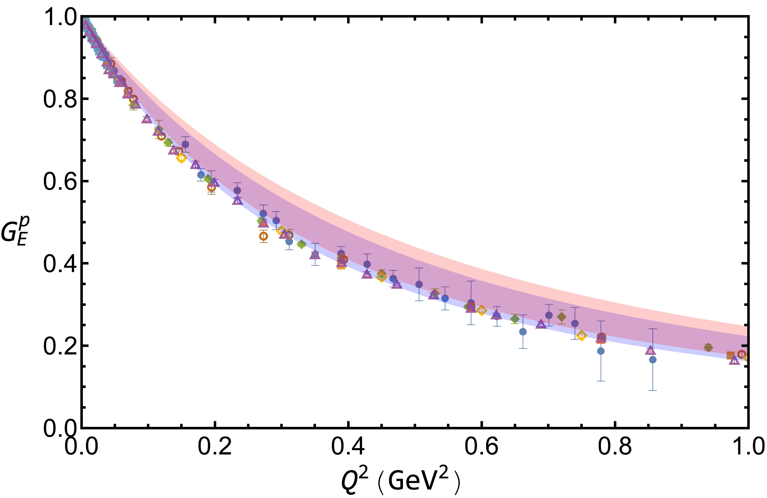
Figure 2. (color online) Electric form factor of the proton
$ G_{E}^{p}(Q^{2}) $ versus momentum transfer$ Q^2 $ with$ \Lambda=1.0 \pm 0.1 $ GeV. The blue and red bands are for the results with and without bubble and tadpole diagrams, respectively.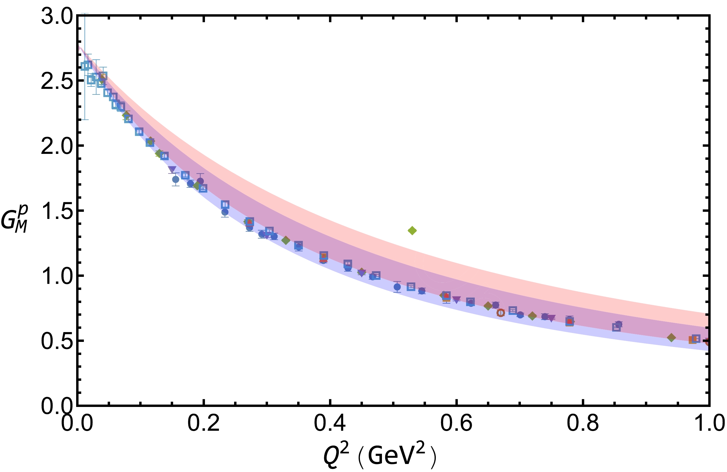
Figure 3. (color online) Same as Fig. 2 but for the magnetic form factor.
As in the proton case, the electromagnetic form factors of the neutron,
$ G_{E}^{n}(Q^{2}) $ and$ G_{M}^{n}(Q^{2}) $ , are plotted in Fig. 4 and Fig. 5. For$ G_E^n(Q^2) $ , both bands first increase and then smoothly decrease with the increasing momentum transfer. The shapes are both comparable with the experimental data. The band with bubble and tadpole contributions is higher than that without those contributions. Obviously, the bubble and tadpole contributions make the theoretical result more reasonable. With the additional diagrams, the neutron charge is 0 at$ Q^2=0 $ . We should mention that the neutron electric form factor in the case without bubble and tadpole diagrams is larger than our previous result [38]. This is mainly because the parameters are a little different. In particular, here the cutoff Λ is chosen to be approximately 1.0 GeV, while it is 0.85 GeV in Ref. [38]. For$ G_M^n(Q^2) $ , there is a slight difference between these two bands, although both of them can describe the experimental data well.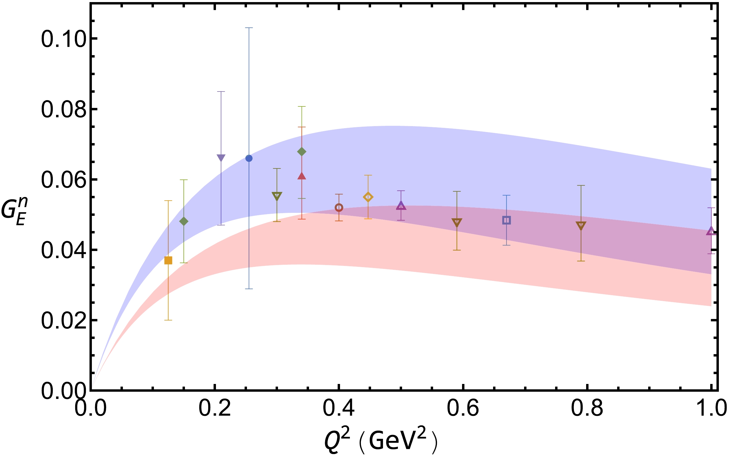
Figure 4. (color online) Electric form factor of the neutron
$ G_{E}^{n}(Q^{2}) $ versus momentum transfer$ Q^2 $ with$ \Lambda=1.0 \pm 0.1 $ GeV. The blue and red bands are for the results with and without bubble and tadpole diagrams, respectively.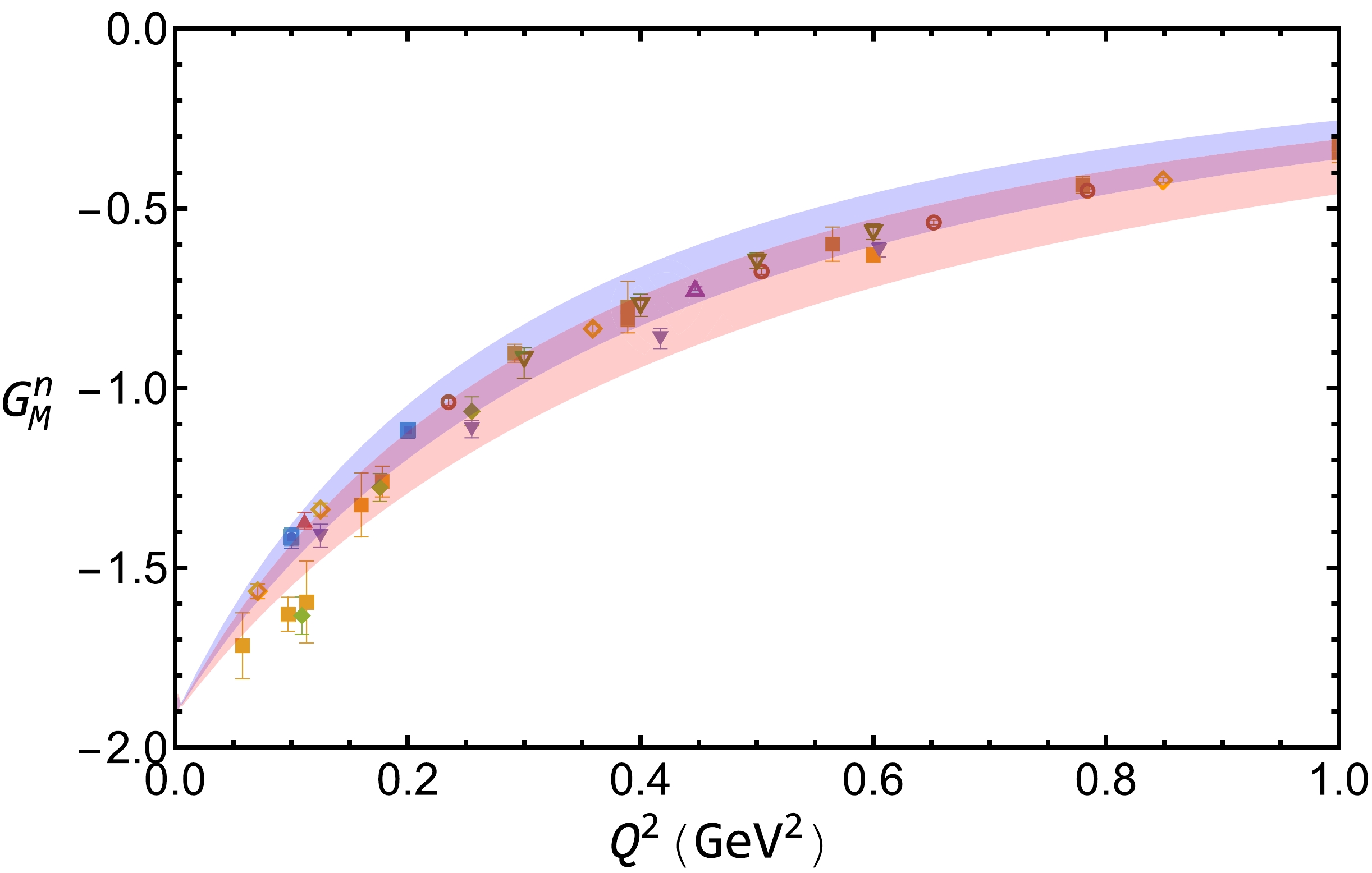
Figure 5. (color online) Same as Fig. 4 but for the magnetic form factor.
From the above numerical results, one can see that for the electromagnetic form factors, even though the determined low energy constants
$ c_1 $ and$ c_2 $ are different, the calculated results with and without bubble and tadpole contributions are both comparable with the experimental data. With the determined parameters, we then present the results for the strange form factors.The strange electric form factor of the nucleon,
$ G_{E}^{s}(Q^{2}) $ , for Λ$ 1.0 \pm 0.1 $ GeV is shown in Fig. 6. As for the nucleon electromagnetic case, the blue and red bands are for the results with and without bubble and tadpole contributions, respectively. The lattice data from Ref. [31] are also shown. In both cases, the strange electric form factor first increases from zero and then changes smoothly with the increasing$ Q^2 $ . The numerical difference of these two cases is obvious. The result with the bubble and tadpole contributions is much larger than that without these contributions. For example, at$ Q^2=0.22 $ GeV$ ^2 $ ,$ G_E^s $ (0.22 GeV$ ^2 $ )$ = 0.0085_{-0.0037}^{+0.0046} $ , which is approximately four times larger than the strange electric form factor without bubble and tadpole contributions. This is because the contributions from the bubble and tadpole diagrams are much larger than those from the diagrams with octet and decuplet intermediate states. We should mention that after we fixed the parameters$ c_1 $ and$ c_1 $ by the magnetic moments of the proton and neutron, the strange form factors are calculated directly without any parameter. Although our values are larger than those of the lattice simulation at finite$ Q^2 $ , the numbers are consistent with the global analysis where$ G_E^{s,\text{exp}}(0.22\; \text{GeV}^2) $ $ =0.035\pm 0.030 \pm 0.019 $ [51].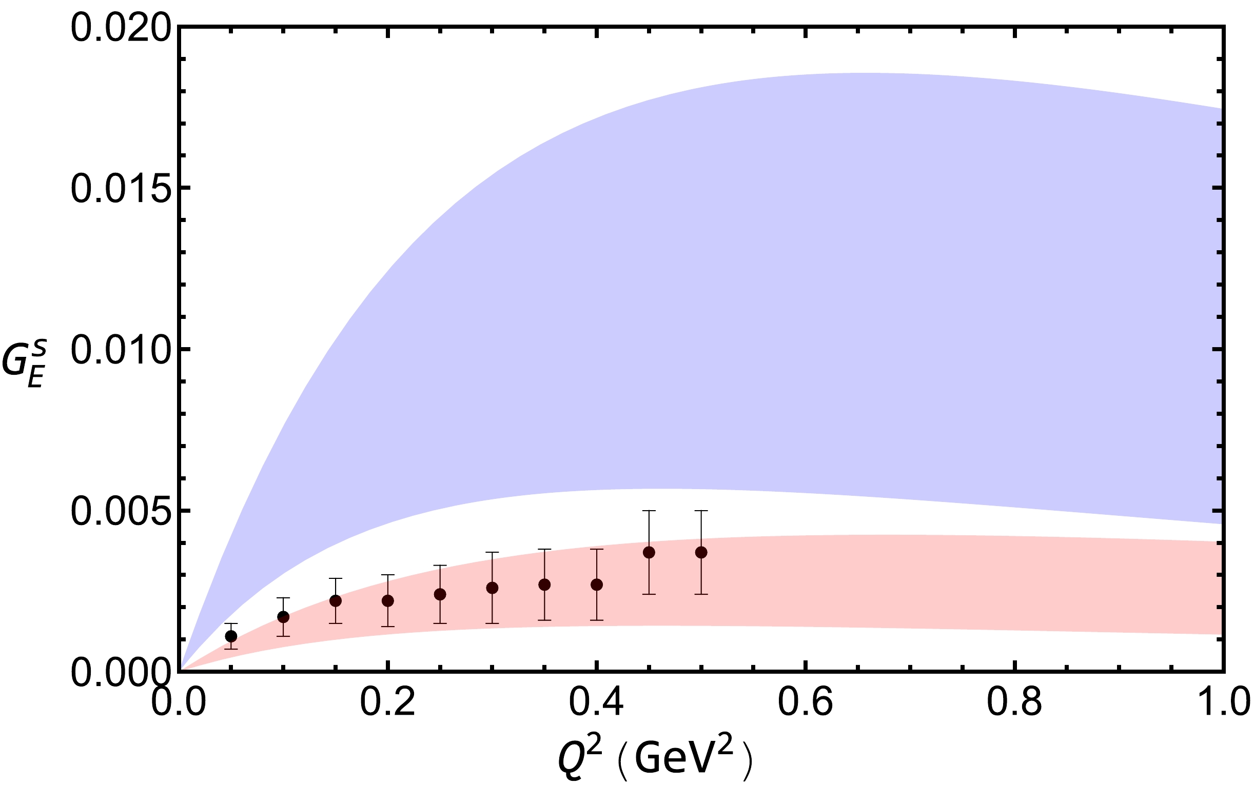
Figure 6. (color online) Strange electric form factor of the nucleon
$ G_{E}^{s}(Q^{2}) $ versus momentum transfer$ Q^2 $ with$ \Lambda=1.0 \pm 0.1 $ GeV. The blue and red bands are for the results with and without bubble and tadpole diagrams, respectively. The lattice data are from Ref. [31].The strange magnetic form factor is plotted in Fig. 7 for the two cases together with the lattice data. For the magnetic case, the contributions from bubble and tadpole diagrams are comparable with those from the rainbow and Kroll-Rudderman diagrams. As a result, the two bands are both negative and comparable. The strange magnetic moment with bubble and tadpole contribution is
$ \mu_s = -0.066_{-0.034}^{+0.028} $ , which is also covered by the experimental analysis$ \mu_s^{\text{exp}} = -0.14 \pm 0.11 \pm 0.11 $ [51].
Figure 7. (color online) Same as Fig. 6 but for the magnetic form factor.
-
We applied the nonlocal EFT to calculate the electromagnetic and strange form factors of the nucleon. The bubble and tadpole diagrams were included in the calculation. The next-to-leading order baryon-meson interaction
$ {\cal L}^{(2)} $ was necessary, even though it was not needed in the previous calculation with only rainbow and Kroll-Rudderman diagrams. In the numerical calculation, all the parameters were predetermined except the cutoff parameter Λ in the regulator and the low energy constants$ c_1 $ and$ c_2 $ .$ c_1 $ and$ c_2 $ were fixed by the nucleon magnetic moments, and Λ was selected to be approximately 1.0 GeV. The numerical results showed that the electromagnetic form factors with and without bubble and tadpole diagrams were close to each other with the proper choices of$ c_1 $ and$ c_2 $ . In both cases, the electromagnetic form factors were in good agreement with the experimental data. As there was no free parameter when we calculated the strange form factors, the obtained strange form factors could have a significant difference in the two cases. With the bubble and tadpole diagrams, the magnitudes of the strange electric and magnetic form factors were both larger. The obtained magnetic moment is$ \mu_s =-0.066_{-0.034}^{+0.028} $ . The strange electric form factor is positive, and$ G_E^s $ (0.22 GeV$ ^2 $ )$ = 0.0085_{-0.0037}^{+0.0046} $ when$ Q^2=0.22 $ GeV$ ^2 $ . Our results revealed that the magnitudes of the strange form factors are larger than the lattice data.
Contributions to the nucleon form factors from bubble and tadpole diagrams
- Received Date: 2022-10-17
- Available Online: 2023-02-15
Abstract: The nonlocal chiral effective theory is applied to investigate the electromagnetic and strange form factors of nucleons. The bubble and tadpole diagrams are included in the calculation. With the contributions from bubble and tadpole diagrams, the obtained electromagnetic form factors are close to the results without these contributions as long as the low energy constants


 DownLoad: