Loading [MathJax]/jax/element/mml/optable/SuppMathOperators.js

Production of Xcsˉcˉs in heavy ion collisions

  • The yields of Xcsˉcˉs with its two possible configurations, i.e., the hadronic molecular state and tetraquark state, for Pb-Pb collisions at sNN=5.02TeV is studied. A volume effect is found from the centrality distribution of Xcsˉcˉs, which could help to distinguish the inner structure of Xcsˉcˉs. We also show the rapidity and the transverse momentum distributions of Xcsˉcˉs production as well as its elliptic flow coefficient as a function of the transverse momentum.
  • Einstein-Gauss-Bonnet (EGB) gravity is the simplest case of Lovelock's extension of Einstein gravity [1]. The theory exists naturally in higher dimensions and becomes important with the development of string theory. Its black hole solutions [2-5] play an important role in studying anti-de Sitter/conformal field theory (AdS/CFT) correspondence. In four dimensions, the Gauss-Bonnet combination is a topological invariant and does not affect the classical equations of motion. Einstein's general relativity is widely believed to be the unique Lagrangian theory yielding second order equations of motion for the metric in four dimensions. The Lovelock type of construction requires additional scalar or vector fields, giving rise to Hordenski gravities [6] or generalized Galilean gravities [7-9].

    However, this has been recently challenged by a novel four dimensional EGB solution [10], which is encoded in the dimensional regularization. After a rescaling of the coupling constant ααD4, the D4 limit can be taken smoothly at the solution level, yielding a nontrivial new black hole. This created a great deal of interest [11-40], as well as controversy [41], as one would expect that higher-derivative theories of finite order that are ghost free in four-dimensions cannot be pure metric theories but are of the Hordenski type. In fact, the resolution of the divergence at the action level is far less clear, and the action principle for the D=4 solution is not given in [10]. One consistent approach is to consider a compactification of D-dimensional EGB gravity on a maximally symmetric space of (Dp) dimensions, where p, keeping only the breathing mode characterizing the size of the internal space such that the theory is minimum. The D\rightarrow p limit can then be smoothly applied [42], leading to an action principle admitting the four dimensional EGB solution [10, 43, 44] (see also [45, 46]). In fact, the analogous D\rightarrow 2 limit of Einstein gravity was proposed many years ago [47] (see also the recent work in [48, 49]). It turns out that the resulting theory is indeed a special Horndeski theory. The action contains a Horndeski scalar that coupled to the Gauss-Bonnet term, as well as the metric field. The lower dimensional action is given by [42]

    \begin{aligned}[b] S_p =& \int {\rm d}^p x \sqrt{-g} \Big[R + \alpha \phi {\cal G} + \alpha \big( 4 G^{\mu\nu} \nabla_\mu \phi \nabla_\nu \phi \\&- 4 (\nabla \phi)^2 \nabla^2 \phi+ 2(\nabla \phi)^2(\nabla \phi)^2 \big) \Big], \end{aligned}

    (1)

    where G^{\mu\nu} is the Einstein tensor, and

    {\cal G}\equiv R^{\mu\nu\rho\sigma}R_{\mu\nu\rho\sigma} - 4 R^{\mu\nu} R_{\mu\nu } + R^2

    (2)

    is the Gauss-Bonnet term.

    There are several interesting features in the new theory (1.1). First, there is no scalar kinematic term; thus, a scalar propagator should be absent. Second, the classical solution of the Minkowski vacuum admits two independent scalar solutions, namely, \phi = 0 , which we refer to as the ordinary vacuum, and \phi = \log \frac{r}{r_0} , which we refer to as the logarithm vacuum. Last but not the least, the \alpha correction is inherited from the higher-dimensional counterparts. Hence, it includes not only the four dimensional Gauss-Bonnet term coupled with a scalar field but also scalar terms that are non-minimally coupled to gravity. The latter seems to be more significant than the former in the corrections to the classical solution of Einstein gravity.

    To test the above interesting features, we will study the asymptotic structure of the lower dimensional EGB theory (1.1) in the Bondi-Sachs framework [50, 51] in the present work. In 1960s, Bondi et al. established an elegant framework of asymptotic expansions to understand the gravitational radiation in axisymmetric isolated systems in the Einstein theory [50]. The metric fields are expanded in inverse powers of a radius coordinate in a suitable coordinate system, and the equations of motion are solved order by order with respect to proper boundary conditions. In this framework [50], the radiation is characterized by a single function from the expansions of the metric fields, which is called the news function. Meanwhile, the mass of the system always decreases whenever there is a news function. Sachs then extended this framework to asymptotically flat spacetime [51]. This is a good starting point to study the asymptotic structure of the theory (1.1) in three dimensions. We obtain the asymptotic form of the solution space. There is no news function in three dimensions. This is a direct demonstration that there is no scalar propagating degree of freedom. Next, we turn to the four dimensional case. Two scalar solutions of the vacuum lead to two different boundary conditions for the scalar fields. The solution spaces are obtained in series expansions with respect to different boundary conditions. For both cases, there is no news function in the expansion of the scalar field, which means that a scalar propagating degree of freedom does not exist in four dimensions. In addition, the \alpha corrections are transparent in the solution space. They arise just one order after the integration constants and also arise in the quadrupole, i.e., the first radiating source in the multipole expansion. In the logarithm vacuum, the \alpha corrections even live at the linearized level. We show the precise formula of the \alpha corrections in the quadrupole. Hence, the two different vacua are indeed experimentally distinguishable.

    The organization of this paper is quite simple. In the next section, we study the asymptotic structure in three dimensions. We perform the same analysis in four dimensions in Section II, with special emphasis on \alpha corrections in the gravitational solutions and the classical radiating source. After a brief conclusion and a discussion on some future directions, we complete the article with an appendix, where some useful relations are listed.

    As a toy model, it is worthwhile to examine the EGB theory (1.1) in three dimensions to determine if the Bondi-Sachs framework is applicable to this theory. In three dimensions, the Gauss-Bonnet term is identically zero. Applying the relations in Appendix A, the variation of the action is obtained as

    \begin{aligned}[b] \delta S_3 =& \int {\rm d}^3 x \sqrt{-g}\bigg\{-\frac12 g_{\tau\gamma}\delta g^{\tau\gamma} \bigg[R + \alpha \big( 4 G^{\mu\nu} \nabla_\mu \phi \nabla_\nu \phi - 4 (\nabla \phi)^2 \nabla^2 \phi + 2(\nabla \phi)^2(\nabla \phi)^2 \big) \bigg] + R_{\mu\nu} \delta g^{\mu\nu} + \nabla_\mu \left(g_{\alpha\beta} \nabla^\mu \delta g^{\alpha\beta} - \nabla_\nu \delta g^{\mu\nu}\right)\\& + \alpha \bigg[2 \left(g_{\rho\sigma} \nabla^\mu \nabla^\nu \delta g^{\rho\sigma} - \nabla_\rho \nabla^\mu \delta g^{\rho\nu} - \nabla_\rho \nabla^\nu \delta g^{\rho\mu} + \nabla^2 \delta g^{\mu\nu} \right) \nabla_\mu \phi \nabla_\nu \phi+ 4 R^\mu_\rho \nabla_\mu\phi \nabla_\nu\phi \delta g^{\nu\rho} + 4 R^\nu_\rho \nabla_\mu\phi \nabla_\nu\phi \delta g^{\mu\rho} \\ & - 2 \bigg( R \nabla_\mu \phi \nabla_\nu \phi \delta g^{\mu\nu} + (\nabla \phi)^2 R_{\rho\sigma} \delta g^{\rho\sigma} + g_{\rho\sigma} (\nabla \phi)^2 \nabla^2 \delta g^{\rho\sigma} - (\nabla \phi)^2 \nabla_\rho \nabla_\sigma \delta g^{\rho\sigma} \bigg)- 4 \delta g^{\mu\nu} \nabla_\mu \phi \nabla_\nu \phi \nabla^2 \phi \\ &- 4 (\nabla \phi)^2 \nabla_\rho \nabla_\sigma \phi \delta g^{\rho\sigma} + 4 \delta g^{\mu\nu} \nabla_\mu \phi \nabla_\nu \phi (\nabla \phi)^2 + 2 (\nabla \phi)^2 g_{\mu\nu} \nabla_\rho \phi \nabla^\rho \delta g^{\mu\nu} - 4 (\nabla \phi)^2 \nabla_\rho \phi \nabla_\mu \delta g^{\rho\mu} \bigg] \\ &+ \alpha \bigg[ 8 G^{\mu\nu} \nabla_\mu \delta \phi \nabla_\nu \phi - 8 g^{\mu\nu} \nabla_\mu \delta \phi \nabla_\nu \phi \nabla^2 \phi + 8 g^{\mu\nu} \nabla_\mu \delta \phi \nabla_\nu \phi (\nabla \phi)^2 - 4 (\nabla \phi)^2 \nabla^2 \delta \phi \bigg]\bigg\}. \end{aligned}

    (3)

    After dropping many boundary terms, one obtains the Einstein equation

    G_{\mu\nu} - \alpha T_{\mu\nu} = 0,

    (4)

    where

    \begin{aligned}[b] T_{\mu\nu} =& g_{\mu\nu} \big[ 4 R^{\rho\sigma} \nabla_\rho \phi \nabla_\sigma \phi + 2 \nabla_\sigma \nabla_\rho \phi \nabla^\rho \nabla^\sigma \phi - 2 (\nabla^2\phi)^2 + (\nabla \phi)^2(\nabla \phi)^2 + 4 \nabla_\rho\nabla_\sigma\phi \nabla^\rho\phi \nabla^\sigma \phi \big]\\ &+ 4 \nabla_\mu \nabla_\nu \phi \nabla^2 \phi - 4 \nabla_\rho\nabla_\mu \phi \nabla^\rho \nabla_\nu \phi + 4 \nabla_\mu \phi \nabla_\nu \phi \nabla^2 \phi - 4 \nabla_\rho \nabla_\mu \phi \nabla_\nu \phi \nabla^\rho \phi - 4 \nabla_\rho \nabla_\nu \phi \nabla_\mu \phi \nabla^\rho \phi \\&- 4 \nabla_\mu \phi \nabla_\nu \phi (\nabla\phi)^2 - 4 R^\rho_\nu \nabla_\mu \phi \nabla_\rho \phi - 4 R^\rho_\mu \nabla_\nu \phi \nabla_\rho \phi +2 R \nabla_\mu \phi \nabla_\nu \phi + 2 G_{\mu\nu} (\nabla \phi)^2 - 4 R_{\mu\rho\nu\sigma}\nabla^\rho \phi \nabla^\sigma \phi , \end{aligned}

    (5)

    and the scalar equation

    G^{\mu\nu} \nabla_\mu \nabla_\nu \phi + R^{\mu\nu} \nabla_\mu \phi \nabla_\nu \phi + \nabla^2\phi (\nabla \phi)^2 - (\nabla^2\phi)^2\\ + 2 \nabla_\rho \nabla_\sigma \phi \nabla^\sigma\phi \nabla^\rho \phi + \nabla_\rho \nabla_\sigma \phi \nabla^\sigma \nabla^\rho \phi = 0.

    (6)

    In order to study three dimensional Einstein theory at future null infinity, the Bondi gauge was adapted to three dimensions with the gauge fixing ansatz [52, 53]

    {\rm d}s^2 = \frac{V}{r} {\rm e}^{2\beta} {\rm d}u^2 - 2 {\rm e}^{2\beta} {\rm d}u{\rm d}r + r^2 ({\rm d}\phi - U {\rm d}u)^2,

    (7)

    in (u,r,\varphi) coordinates, and \beta,U,V are functions of (u,r,\varphi) . Suitable fall-off conditions that preserve asymptotic flatness are

    U = {\cal O}(r^{-2}),\quad V = {\cal O}(r), \quad \beta = {\cal O}(r^{-1}),\quad \phi = {\cal O}(r^{-1}).

    (8)

    One of the advantages of the Bondi gauge is encoded in the organization of the equations of motion [50, 51, 53] (also see [54, 55] for the generalization to matter coupled theories). There are four types of equations of motion, namely the main equation, standard equation, supplementary equation, and trivial equation. The terminology characterizes their special properties. The main equations determine the r-dependence of the unknown functions \beta,U,V , while the standard equation controls the time evolution of the scalar field. Because of the Bianchi identities, the supplementary equations are left with only one order in the 1/r expansion undetermined, and the trivial equation is fulfilled automatically when the main equations and the standard equation are satisfied. In three dimensional EGB theory (1.1), the components G_{rr} - \alpha T_{rr} = 0 , G_{r\varphi} - \alpha T_{r\varphi} = 0 , and G_{ru} - \alpha T_{ru} = 0 are the main equations. The scalar equation is the standard equation; G_{u\varphi} - \alpha T_{u\varphi} = 0 and G_{uu} - \alpha T_{uu} = 0 are the supplementary equations. Finally, G_{\varphi\varphi} - \alpha T_{\varphi\varphi} = 0 is the trivial equation.

    Once the scalar field is given as initial data in the series expansion

    \phi(u,r,\varphi) = \sum_{a = 1}^\infty\frac{\phi_a(u,\varphi)}{r^a},

    (9)

    the unknown functions \beta,U,V can be solved explicitly. In asymptotic form, they are

    \begin{aligned}[b] \beta =& \frac{3 \alpha \phi_1 \partial_u \phi_1}{4r^3} + \frac{\alpha}{2r^4} \bigg[ 2M \phi_1^2 + 4 (\partial_\varphi \phi_1)^2 - 2 \phi_1 \partial_\varphi^2 \phi_1\\& + 5 \phi_1^2 \partial_u \phi_1 + 6 \phi_2 \partial_u\phi_1 + 2 \phi_1 \partial_u \phi_2 \bigg] + {\cal O}(r^{-5}), \end{aligned}

    (10)

    \begin{aligned}[b] U =& \frac{N(u,\varphi)}{r^2} - \frac{\alpha}{6r^4}\bigg[20 \partial_u\phi_1 \partial_\varphi \phi_1 + \phi_1 \left(3 \partial_\varphi M \partial_u \phi_1 \right.\\&\left.- \partial_u N \partial_u \phi_1 - 4 \partial_u\partial_\varphi \phi_1\right)\bigg] + {\cal O}(r^{-5}), \end{aligned}

    (11)

    \begin{aligned}[b] V =& -r M(u,\varphi) - \frac1r\left[ N^2 - 2 \alpha \partial_u \phi_1 (2\partial_u\phi_1 - \phi_1 \partial_u M)\right]\\ & + \frac{\alpha}{3r^2} \bigg[4(1-M) \phi_1^2 \partial_u M - 8 \phi_2 \partial_u \phi_1 \partial_u M - 4 \phi_1 \partial_u \phi_2 \partial_u M\\ & + \partial_\varphi M \partial_\varphi \phi_1 \partial_u \phi_1 - 2 \partial_\varphi \phi_1 \partial_u N \partial_u \phi_1- 4 \partial_\varphi^2 \phi_1 \partial_u \phi_1 \\ &+ 24 \partial_u \phi_1 \partial_u \phi_2+ 16 \partial_\varphi \phi_1 \partial_u\partial_\varphi \phi_1 + \phi_1 \bigg(16 M \partial_u \phi_1 \\ &- 3 \partial_\varphi M \partial_u \phi_1 + 8 (\partial_u \phi_1)^2 + 6 \partial_u \phi_1 \partial_u\partial_\varphi N + \partial_\varphi M \partial_u \partial_\varphi \phi_1 \\ &- 2 \partial_u N \partial_u\partial_\varphi \phi_1 - 4 \partial_u\partial_\varphi^2 \phi_1 \bigg)\bigg] + {\cal O}(r^{-3}), \\[-15pt]\end{aligned}

    (12)

    where N(u,\varphi) and M(u,\varphi) are integration constants. Compared to the pure Einstein case [53], the \alpha corrections are at least two orders after the integration constants. The solution space is no longer in a closed form.

    The time evolution of every order of the scalar field is controlled from the standard equation. This means that there is no news function from the scalar field. We list the first two orders of the standard equation

    2(\partial_u \phi_1)^2 + \phi_1 (\partial_u M + 4 \partial_u^2 \phi_1 ) = 0 ,

    (13)

    \begin{aligned}[b]&4\partial_u (\phi_1 \partial_u \phi_2) + 8 \partial_\varphi \phi_1 \partial_u\partial_\varphi \phi_1 + 12 \phi_2 \partial_u^2 \phi_1 + 2 \phi_1^2 \partial_u^2 \phi_1 -4 \partial_\varphi^2 \phi_1 \partial_u \phi_1 + \phi_1 \left(\partial_\varphi^2 M + 8 M \partial_u \phi_1 + 10 (\partial_u \phi_1)^2 - 2 \partial_u\partial_\varphi N\right) \\&\quad - 2 \partial_\varphi M \partial_\varphi \phi_1 + 4 \partial_\varphi \phi_1 \partial_u N + \frac52 \phi_1^2 \partial_u M + 3 \phi_2 \partial_u M = 0 . \end{aligned}

    (14)

    The constraints from the supplementary equations are

    \partial_u M = 0,

    (15)

    \partial_u N = \frac12 \partial_\varphi M,

    (16)

    which are the same as in the pure Einstein case. This is well expected, as the \alpha corrections are in the higher orders. In the end, there is no propagating degree of freedom at all in this theory in three dimensions. The whole effect of the higher dimensional Gauss-Bonnet terms is a kind of deformation of Einstein gravity.

    We now turn to the more realistic case of four dimensions. The action is given by (1.1) with p = 4 . The derivation of the equations of motion is quite similar to the three dimensional case, with the additional contribution from the Gauss-Bonnet term, which is detailed in Appendix A. The Einstein equation is obtained as

    G_{\mu\nu} - \alpha T_{\mu\nu} = 0,

    (17)

    where the modification to T_{\mu\nu} (5) from the Gauss-Bonnet term is

    \begin{aligned}[b] &-4 R_{\mu\rho\nu\sigma}\nabla^\rho \nabla^\sigma \phi + 4 G_{\mu\nu} \nabla^2 \phi - 4 R_\mu^\rho \nabla_\nu \nabla_\rho \phi - 4 R_\nu^\rho \nabla_\mu \nabla_\rho \phi\\& + 4 g_{\mu\nu} R^{\rho\sigma} \nabla_\rho \nabla_\sigma \phi + 2 R \nabla_\mu\nabla_\nu \phi ,\end{aligned}

    (18)

    and the scalar equation is

    \begin{aligned}[b] &G^{\mu\nu} \nabla_\mu \!\nabla_\nu \!\phi \!+\! R^{\mu\nu} \!\nabla_\mu\! \phi \!\nabla_\nu \!\phi \!+\! \nabla^2\phi (\nabla \!\phi)^2 \!-\! (\nabla^2\!\phi)^2 \!+\! 2 \!\nabla_\rho \!\nabla_\sigma \!\phi \nabla^\sigma\!\phi \!\nabla^\rho \!\phi \\ & \quad + \nabla_\rho \nabla_\sigma \phi \nabla^\sigma \nabla^\rho \phi - \frac18 \left(R^{\mu\nu\rho\sigma}R_{\mu\nu\rho\sigma} - 4 R^{\mu\nu} R_{\mu\nu } + R^2\right) = 0. \end{aligned}

    (19)

    In four dimensions, we choose the Bondi gauge fixing ansatz [50]

    \begin{aligned}[b] {\rm d}s^2 =& \left[\frac{V}{r}{\rm e}^{2\beta} + U^2r^2{\rm e}^{2\gamma}\right]{\rm d}u^2 - 2{\rm e}^{2\beta}{\rm d}u{\rm d}r\\ &- 2U r^2{\rm e}^{2\gamma}{\rm d}u{\rm d}\theta + r^2\left[{\rm e}^{2\gamma}{\rm d}\theta^2 + {\rm e}^{-2\gamma}\sin^2\theta {\rm d}\phi^2\right], \end{aligned}

    (20)

    in (u,r,\theta,\varphi) coordinates. The metric ansatz involves four functions (V,U,\beta,\gamma) of (u,r,\theta) that are to be determined by the equations of motion. These functions and the scalar field are \varphi -independent, and hence, the metric has manifest global Killing direction \partial_\varphi . This is the “axisymmetric isolated system” introduced in [50]. Following [50] closely, the falloff conditions for the functions (\beta,\gamma,U,V) in the metric for asymptotic flatness are given by

    \beta = {\cal O}(r^{-1}),\;\;\;\;\gamma = {\cal O}(r^{-1}),\;\;\;\;U = {\cal O}(r^{-2}),\;\;\;\;V = -r + {\cal O}(1).

    (21)

    Considering the metric of the Minkowski vacuum

    {\rm d}s^2 = -{\rm d}u^2-2{\rm d}u{\rm d}r+r^2({\rm d}\theta^2 + \sin^2\theta {\rm d}\phi^2),

    (22)

    we have two branches of the scalar solution

    \phi = 0,\quad {\rm{or}} \quad \phi = \log \frac{r}{r_0}.

    (23)

    The first gives the true vacuum with the maximal spacetime symmetry preserved; the second solution is nearly Minkowski, since the scalar does not preserve the full symmetry. Both are valid solutions, with one not encompassing the other. Analogous emergence of logarithmic dependence for the scalar also occurs in the AdS vacuum for some critical Einstein-Horndeski gravity, where the scalar breaks the full conformal symmetry of the AdS to the subgroup of the Poincare together with the scaling invariance [56]. However, ours is the first example in the Minkowski vacuum. The necessary falloff condition of the scalar field consistent with the metric falloffs is either

    \phi = {\cal O}(r^{-1}),\quad {\rm{or}}\quad \phi = \log \frac{r}{r_0} + {\cal O}(r^{-1}).

    (24)

    Similar to the three-dimensional case, the equations of motion are organized as follows: G_{rr} - \alpha T_{rr} = 0 , G_{r\theta} - \alpha T_{r\theta} = 0 , and G_{\theta\theta}g^{\theta\theta} + G_{\varphi\varphi}g^{\varphi\varphi} - \alpha T_{\theta\theta} g^{\theta\theta} - \alpha T_{\varphi\varphi} g^{\varphi\varphi} = 0 are the main equations. The scalar equation and G_{\theta\theta} - \alpha T_{\theta\theta} = 0 are the standard equations; G_{u\theta} - \alpha T_{u\theta} = 0 and G_{uu} - \alpha T_{uu} = 0 are supplementary; and G_{ru} - \alpha T_{ru} = 0 is trivial. G_{r\varphi} - \alpha T_{r\varphi} = 0 , G_{\theta\varphi} - \alpha T_{\theta\varphi} = 0 , and G_{u\varphi} - \alpha T_{u\varphi} = 0 are trivial because the system is \varphi -independent.

    Suppose that \gamma and \phi are given in a series expansion as initial data

    \gamma = \frac{c(u,\theta)}{r} + \sum^{\infty}_{a = 3}\frac{\gamma_a(u,\theta)}{r^a},

    (25)

    \phi = \sum^{\infty}_{a = 1}\frac{\phi_a(u,\theta)}{r^a}.

    (26)

    The unknown functions \beta,U,V are solved in asymptotic form as

    \beta = -\frac{c^2}{4r^2} + \frac{4 \alpha \phi_1 \partial_u \phi_1}{3r^3} + {\cal O}(r^{-4}),

    (27)

    \begin{aligned}[b] U =& -\frac{2\cot\theta c + \partial_\theta c}{r^2} + \frac{N(u,\varphi)}{r^3} + \frac{1}{2r^4}\bigg[5 \cot\theta c^3 - 3c N \\&+ 6 \cot\theta \gamma_3 + \frac52 c^2 \partial_\theta c + 3 \partial_\theta c + \alpha\Bigg( 16 \cot\theta \phi_1 \partial_u c \\ &\left.- \frac{20}{3} \partial_\theta \phi_1 \partial_u \phi_1 + 8 \phi_1 \partial_u\partial_\theta c + \frac43 \phi_1 \partial_u\partial_\theta \phi_1\right) \bigg] + {\cal O}(r^{-5}), \end{aligned}

    (28)

    \begin{aligned}[b] V \!=\!& -r \!+\! M(u,\theta) \!+\! \frac{1}{2r}\bigg[ \cot\theta N \!-\! \frac12 c^2 (5\!+\!11\cos2\theta)\csc^2\theta\\& \!-\! 5 (\partial_\theta c)^2 + \partial_\theta N - c(19\cot\theta \partial_\theta c + 3 \partial_\theta^2 c) \\& + 8 \alpha (\partial_u\phi_1)^2 \bigg] + {\cal O}(r^{-2}), \end{aligned}

    (29)

    where N(u,\theta) and M(u,\theta) are integration constants. Clearly, the coupling \alpha emerges just one order after the integration constants. They are from the non-minimal coupled scalar rather than the four dimensional Gauss-Bonnet term.

    The standard equations control the time evolution of the initial data \gamma and \phi . In particular, the time evolution of every order of the scalar field has been constrained. That means there is no news function associated to the scalar field. Hence, the scalar field does not have a propagating degree of freedom similar to the three dimensional case. We list the first two orders of the scalar equation

    (\partial_u\phi_1)^2 + \phi_1 \partial_u^2 \phi_1 = 0,

    (30)

    \begin{aligned}[b] &2 \phi_1 \partial_u^2 \phi_2 + 6 \partial_u \phi_1 \partial_u \phi_2 - \partial_\theta^2 \phi_1 \partial_u \phi_1 - \cot\theta \partial_\theta \phi_1 \partial_u \phi_1 + 4 \partial_\theta \phi_1 \partial_u\partial_\theta \phi_1 + \phi_1^2 \partial_u^2 \phi_1 + 6 \phi_2 \partial_u^2 \phi_1 + 6 \phi_1 \partial_u \phi_1 + 4 \phi_1 (\partial_u\phi_1)^2\\&\quad + \phi_1\left[\partial_u\partial_\theta^2 c + 3 \cot\theta \partial_u\partial_\theta c - 2 \partial_u c - 2 (\partial_u c)^2 - \partial_u M \right] = 0.\end{aligned}

    (31)

    The first order of the standard equation from the Einstein equation is

    \begin{aligned}[b] \partial_u \gamma_3 =& \frac18 \bigg[3 (\partial_\theta c)^2 + c (5\cot\theta \partial_\theta c + 3 \partial_\theta^2 c) -2 c^2 \csc^2\theta \\&\times(3 + \cos2\theta) + 2 c M + \cot\theta N - \partial_\theta N - 16 \alpha \phi_1 \partial_u^2 c \bigg]. \end{aligned}

    (32)

    In the Newman-Penrose variables, \gamma_3 is related to \Psi_0^0 or {\bar \Psi }_0^0 [57]. Since its time evolution involves \alpha , the effect of the higher dimensional Gauss-Bonnet term arises, starting from the first radiating source, i.e., quadrupole, in the multipole expansion [58]. This can be seen more precisely on a linearized level from the logarithm vacuum case, which we will present in the next subsection.

    The supplementary equations yield

    \partial_u N = \frac13\left[ 7 \partial_\theta c \partial_u c + c(16\cot\theta \partial_u c + 3 \partial_u\partial_\theta c) - \partial_\theta M \right].

    (33)

    \partial_u m = -2(\partial_u c)^2,\quad m \equiv M - \frac{1}{\sin\theta} \partial_\theta ( 2 \cos\theta c + \sin\theta \partial_\theta c).

    (34)

    The latter is the mass-loss formula in this theory. It is the same as that in the pure Einstein case [50] , which is expected, as the corrections from the Gauss-Bonnet term are in the higher orders.

    One intriguing feature of the theory is that the scalar admits a logarithmic dependence in the Minkowski vacuum, such that the full Lorentz group breaks down for any matter coupled to the scalar. We would like to analyze its solution space here. Suppose that \gamma and \phi are given in series expansions as initial data:

    \gamma = \frac{c(u,\theta)}{r} + \sum^{\infty}_{a = 3}\frac{\gamma_a(u,\theta)}{r^a},

    (35)

    \phi = \log \frac{r}{r_0} + \sum^{\infty}_{a = 1}\frac{\phi_a(u,\theta)}{r^a}.

    (36)

    We can solve the unknown functions \beta,U,V in asymptotic form as

    \begin{aligned}[b] \beta =& -\frac{c^2}{4r^2} + \frac{1}{4r^4}\bigg[-3 c \gamma_3 + \alpha \bigg(4c\cot\theta (\partial_\theta c + \partial_\theta \phi_1 ) + c^2 ( \csc^2\theta + 3 \cot^2\theta) - \phi_1^2 - 2 \phi_2 + (\partial_\theta c)^2 + 2 \partial_\theta c\partial_\theta \phi_1 \\&+ (\partial_\theta \phi_1 )^2 + 2 \alpha \partial_u \phi_1 - 8 \alpha (\partial_u \phi_1 )^3\bigg)\bigg] + {\cal O}(r^{-5}), \end{aligned}

    (37)

    \begin{aligned}[b] U =& -\frac{2\cot\theta c + \partial_\theta c}{r^2} + \frac{N(u,\varphi)}{r^3}+ \frac{1}{2r^4}\bigg\{5 \cot\theta c^3 - 3c N + 6 \cot\theta \gamma_3 + \frac52 c^2 \partial_\theta c + 3 \partial_\theta c + \alpha \bigg[ 14\partial_\theta c \partial_u c \partial_u \phi_1\\& - 4 \partial_\theta c \partial_u c - 4 \partial_\theta \phi_1 \partial_u c - 4 \partial_\theta c \partial_u \phi_1 - 2 \partial_\theta M \partial_u \phi_1 - 6 \partial_u N \partial_u \phi_1\\ & - 2 c \left( 4\cot\theta \partial_u c - 16 \cot\theta \partial_u c \partial_u \phi_1 + 4 \cot\theta \partial_u \phi_1 - 3 \partial_u \partial_\theta c \partial_u \phi_1 \right)\bigg] \bigg\} + {\cal O}(r^{-5}), \end{aligned}

    (38)

    V = -r + M(u,\theta) + \frac{1}{2r}\bigg[ \cot\theta N - \frac12 c^2 (5+11\cos2\theta)\csc^2\theta - 5 (\partial_\theta c)^2 + \partial_\theta N - c(19\cot\theta \partial_\theta c + 3 \partial_\theta^2 c) - 2 \alpha + 8 \alpha (\partial_u\phi_1)^2 \bigg] + {\cal O}(r^{-2}).

    (39)

    The coupling \alpha emerges again one order after the integration constants. At this order, it is from the non-minimally coupled scalar. The \alpha^2 terms in \beta indicate the nonlinear scalar-gravity coupling.

    The time evolution of every order of the scalar field is also constrained. There is no news function associated with the scalar field. The first two orders of the scalar equation are

    \partial_u \phi_1 + (\partial_u \phi_1)^2 - (\partial_u c)^2 - \frac12 = 0,

    (40)

    \begin{aligned}[b]& 4\phi_2 \partial_u^2 \phi_1 - 4 \partial_u \phi_2 - 8 \partial_u \phi_1 \partial_u \phi_2 - 3 M - 2 \phi_1 + 3 \cot\theta \partial_\theta c + \cot\theta \partial_\theta \phi_1 + \partial_\theta^2 c + \partial_\theta^2 \phi_1 - 2 \cot\theta \partial_\theta c \partial_u c + 2 \cot\theta \partial_\theta \phi_1 \partial_u c - 2 \partial_\theta^2 c \partial_u c \\ &\quad- 2 \partial_\theta^2 \phi_1 \partial_u c - 4 \phi_1 (\partial_u c)^2 - 6 \phi_1 \partial_u \phi_1 - 12 \cot\theta \partial_\theta c \partial_u \phi_1 - 4\cot\theta \partial_\theta \phi_1 \partial_u \phi_1 - 4 \partial_\theta^2 c \partial_u \phi_1 - 4 \partial_\theta^2 \phi_1 \partial_u \phi_1 + 8 \phi_1 (\partial_u\phi_1)^2 \\&\quad+ 4 \partial_\theta c \partial_u\partial_\theta \phi_1 + 4 \partial_\theta \phi_1 \partial_u \partial_\theta \phi_1 - 2c + 8 c \partial_u \phi_1+c \partial_u c (8\csc^2\theta - 4 \partial_u \phi_1 ) + 8 \cot\theta c \partial_u \partial_\theta \phi_1 - 2 c^2 \partial_u^2 \phi_1 + 2 \phi_1^2 \partial_u^2 \phi_1 = 0.\end{aligned}

    (41)

    The first order of the standard equation from the Einstein equation is

    \begin{aligned}[b] \partial_u \gamma_3 = &\frac18 \bigg[3 (\partial_\theta c)^2 + c (5\cot\theta \partial_\theta c + 3 \partial_\theta^2 c) \\ & -2 c^2 \csc^2\theta (3 + \cos2\theta)+ 2 c M + \cot\theta N \\ & - \partial_\theta N - 8 \alpha \partial_u c + 16 \alpha \partial_u \phi_1 \partial_u c \bigg]. \end{aligned}

    (42)

    The constraints from the supplementary equations are

    \partial_u N = \frac13\left[ 7 \partial_\theta c \partial_u c + c(16\cot\theta \partial_u c + 3 \partial_u\partial_\theta c) - \partial_\theta M \right].

    (43)

    \partial_u m = -2(\partial_u c)^2,\quad m \equiv M - \frac{1}{\sin\theta} \partial_\theta ( 2 \cos\theta c + \sin\theta \partial_\theta c).

    (44)

    The mass-loss formula is the same as that for the pure Einstein case [50].

    To reveal the \alpha correction in the radiating source, we linearize the theory, for which we drop all the quadratic terms in the solutions. Then, the evolution equations are reduced to

    \partial_u M = \frac{1}{\sin\theta} \partial_\theta\left[\frac{1}{\sin\theta} \partial_\theta \left(\sin^2\theta \partial_u c\right)\right],

    (45)

    \partial_u N = -\frac13 \partial_\theta M,

    (46)

    \partial_u \gamma_3 = - \frac18 \sin\theta \partial_\theta \frac{N}{\sin\theta} - \alpha \partial_u c.

    (47)

    The \alpha correction is now only from the scalar background \log \frac{r}{r_0} term. The multipole expansion is encoded in the expansion of \gamma [58]. The quadrupole in Eq. (2.46) of [58] corresponds to \gamma_3 = a_2(u) \sin^2\theta , where the subscript 2 denotes the second order of the second associated Legendre function. The function c can be solved from the above evolution equations. The solution is c = c_2(u)\sin^2\theta , where c_2(u) satisfies

    c_2-\alpha \partial_u^2 c_2 = \partial_u^2 a_2.

    (48)

    Suppose that a_2 is a periodic function, e.g., a_2 = A \sin u + B \cos u . Then the response of c_2 will have an \alpha correction c_2 = \dfrac{\partial_u^2 a_2}{1+\alpha} . By setting \alpha = 0 , we just recover the Einstein gravity result c = \partial_u^2 a_2 \sin^2\theta . For the same type of gravitational source, the new theory (1.1) is indeed distinguishable from Einstein gravity. Since the c function has a direct connection to the Weyl tensor [57], we can expect a direct experimental test of the \alpha corrections.

    In this paper, the asymptotic structures of three and four dimensional EGB gravity have been studied in the Bondi-Sachs framework. It was shown from the solution space that, in both dimensions, there is no scalar propagator. The \alpha corrections were discussed in detail from the perspective of both the gravitational solution and radiating sources.

    There are several open questions in the theory (1.1) that should be addressed in the future. There is no scalar propagator in the theory, but there are differential couplings between gravity and the scalar field. The absence of the scalar propagator is likely to be consistent with observations; thus, it is of interest to know how to construct a gravity-scalar vertex without a scalar propagator [59]. A second interesting point is from the holography. In three dimensions, asymptotically flat gravitational theory has a holographic dual description [53, 60]. It would be very meaningful to explore the dual theory of the three dimensional EGB gravity. Another question worth mentioning is from the recent proposal of a triangle equivalence [61]. Since the change in the c function has \alpha corrections for the same type of gravitational source, the gravitational memory receives the \alpha correction [62]. In the context of the triangle relation, it is a very interesting question as to whether the soft graviton theorem and the asymptotic symmetry have \alpha corrections as well.

    The authors thank Yue-Zhou Li and Xiaoning Wu for useful discussions.

    We list some useful relations that may help readers who are less familiar with the variational principle involving the Gauss-Bonnet term.

    The Bianchi identity is given by

    \tag{A1} \nabla_\mu {R_{\nu\sigma\rho}}^\nu + \nabla_\nu {R_{\sigma\mu\rho}}^\nu + \nabla_\sigma {R_{\mu\nu\rho}}^\nu = 0.

    The commutator of \nabla :

    \tag{A2} (\nabla_\mu\nabla_\nu - \nabla_\nu\nabla_\mu) S^{\rho\sigma} = {R^{\rho}}_{\tau\mu\nu} S^{\tau\sigma} + {R^{\sigma}}_{\tau\mu\nu} S^{\rho\tau}.

    Variations of some relevant quantities are as follows:

    \tag{A3} \delta \sqrt{-g} = -\frac12\sqrt{-g}g_{\mu\nu}\delta g^{\mu\nu},

    \tag{A4} \delta \Gamma^\sigma_{\mu\nu} = -\frac12 \nabla^\sigma \delta g_{\mu\nu} - \frac12g_{\mu\tau}\nabla_\nu \delta g^{\sigma\tau} - \frac12 g_{\nu\tau} \nabla_\mu \delta g^{\sigma\tau},

    \tag{A5} g^{\mu\nu}\delta \Gamma^\sigma_{\mu\nu} = \frac12 g_{\mu\nu} \nabla^\sigma \delta g^{\mu\nu} - \nabla_\mu \delta g^{\sigma\mu},

    \tag{A6} \delta {R^\sigma}_{\mu\rho\nu} = \nabla_\rho \delta \Gamma^\sigma_{\mu\nu} - \nabla_\nu \delta \Gamma^\sigma_{\mu\rho},

    \tag{A7}\begin{aligned}[b] \delta R_{\mu\nu} =& \frac12 \left(g_{\sigma\rho} \nabla_\mu \nabla_\nu \delta g^{\sigma\rho} - g_{\sigma\nu} \nabla_\rho\nabla_\mu \delta g^{\rho\sigma}\right.\\& \left.- g_{\sigma\mu} \nabla_\rho \nabla_\nu \delta g^{\rho\sigma} - \nabla^2 \delta g_{\mu\nu}\right), \end{aligned}

    \tag{A8} \delta R = R_{\mu\nu} \delta g^{\mu\nu} + \nabla_\mu \left(g_{\sigma\rho} \nabla^\mu \delta g^{\sigma\rho} - \nabla_\nu \delta g^{\mu\nu}\right),

    \tag{A9} \begin{aligned}[b] \delta G^{\mu\nu} =& \frac 12 \left(g_{\sigma\rho} \nabla^\mu \nabla^\nu \delta g^{\sigma\rho} - \nabla_\sigma \nabla^\mu \delta g^{\sigma\nu} - \nabla_\sigma \nabla^\nu \delta g^{\sigma\mu}+ \nabla^2 \delta g^{\mu\nu} \right) \\ & + R^\mu_\sigma \delta g^{\nu \sigma} + R^\nu_\sigma \delta g^{\mu \sigma} - \frac12 R \delta g^{\mu\nu} - \frac12 g^{\mu\nu} R_{\sigma\rho} \delta g^{\sigma\rho}\\& - \frac12 g^{\mu\nu}g_{\sigma\rho} \nabla^2 \delta g^{\sigma\rho} + \frac12 g^{\mu\nu} \nabla_\rho \nabla_\sigma \delta g^{\rho\sigma}, \end{aligned}

    \tag{A10} \delta R^2 = 2 R R_{\rho\sigma} \delta g^{\rho\sigma} + 2R \left(g_{\sigma\rho} \nabla^2 \delta g^{\sigma\rho} - \nabla_\mu \nabla_\nu \delta g^{\mu\nu}\right),

    \tag{A11} \delta (R^{\sigma\mu\rho\nu} R_{\sigma\mu\rho\nu}) = 4R_{\sigma\mu\rho\nu}\nabla^\nu\nabla^\mu\delta g^{\rho\sigma} + 2 R_{\sigma\mu\rho\nu} {{R^\sigma}_\tau}^{\rho\nu} \delta g^{\mu\tau},

    \tag{A12} \begin{aligned}[b]\delta (R^{\mu\nu} R_{\mu\nu}) =& R_{\rho\sigma} \nabla^2 \delta g^{\rho\sigma} - R_{\mu\rho} \nabla_\sigma \nabla^\mu \delta g^{\rho\sigma}\\ & + g_{\rho\sigma} R^{\mu\nu} \nabla_\mu \nabla_\nu \delta g^{\rho\sigma} - R^\mu_\sigma \nabla_\mu \nabla_\rho \delta g^{\rho\sigma}\\& + R_{\mu\nu} R^\nu_\sigma \delta g^{\mu\sigma} + R_{\sigma\mu\rho\nu} R^{\mu\nu} \delta g^{\sigma\rho}, \end{aligned}

    \tag{A13}\begin{aligned}[b] g^{\mu\nu} \delta (\nabla_\mu \nabla_\nu \phi) =& g^{\mu\nu} \nabla_\mu \nabla_\nu \delta \phi - \frac12 g_{\mu\nu} \nabla_\sigma \phi \nabla^\sigma \delta g^{\mu\nu} \\&+ \nabla_\sigma \phi \nabla_\mu \delta g^{\sigma\mu}, \end{aligned}

    \tag{A14} \begin{aligned}[b] \delta {\cal G} =& 2 R_{\sigma\mu\tau\nu} {R_\rho}^{\mu\tau\nu} \delta g^{\sigma\rho} + 2 R R_{\rho\sigma} \delta g^{\rho\sigma} - 4 R_{\rho\nu} R^\nu_\sigma \delta g^{\rho\sigma} \\&- 4 R_{\sigma\mu\rho\nu} R^{\mu\nu} \delta g^{\sigma\rho}4 {R_{\sigma\mu\rho}}^\nu \nabla_\nu\nabla^\mu\delta g^{\rho\sigma} + 4 {R_{\nu\sigma\rho}}^\nu \nabla_\mu \nabla^\mu \delta g^{\rho\sigma} \\&+ 4 {R_{\mu\nu\rho}}^\nu \nabla_\sigma \nabla^\mu \delta g^{\rho\sigma} - 4 g_{\rho\sigma} G^{\mu\nu} \nabla_\mu \nabla_\nu \delta g^{\rho\sigma} \\ &+ 4 G^\mu_\rho \nabla_\mu \nabla_\sigma \delta g^{\rho\sigma}. \end{aligned}

    The first line of (A14) equals \dfrac12 g_{\sigma\rho}{\cal G} \delta g^{\sigma\rho} in four dimensions. Thus, they will not contribute to the equations of motion. When performing integration by parts, the second line and the third line vanish automatically for the pure Gauss-Bonnet term. However, it will contribute when the scalar field is coupled to the Gauss-Bonnet term, e.g., \phi{\cal G} . The second line and the third line can be reorganized as follows:

    \tag{A15}\begin{aligned}[b] 4 {R_{\sigma\mu\rho\nu}} \nabla^\nu\nabla^\mu\delta g^{\rho\sigma} &+ 4 {R_{\nu\sigma\rho}}^\nu \nabla_\mu \nabla^\mu \delta g^{\rho\sigma} + 4 R^\mu_\rho \nabla_\sigma \nabla_\mu \delta g^{\rho\sigma}\\& - 4 g_{\rho\sigma} G^{\mu\nu} \nabla_\mu \nabla_\nu \delta g^{\rho\sigma} + 4 R^\mu_\rho \nabla_\mu \nabla_\sigma \delta g^{\rho\sigma}\\& - 2 R \nabla_\sigma\nabla_\rho \delta g^{\rho\sigma}. \end{aligned}

    The point of such reorganization is to make the indexes of the two covariant derivatives in every term symmetric. When integrating by parts for the pure Gauss-Bonnet term, both covariant derivatives are identically zero.

    [1] M. Gell-Mann, Phys. Lett. 8, 214-215 (1964) doi: 10.1016/S0031-9163(64)92001-3
    [2] G. Zweig, CERN-TH-401.
    [3] G. Zweig, CERN-TH-412.
    [4] P. A. Zyla et al. (Particle Data Group), PTEP 2020(8), 083C01 (2020) doi: 10.1093/ptep/ptaa104
    [5] R. Aaij et al. (LHCb), Phys. Rev. Lett. 115, 072001 (2015), arXiv:1507.03414[hep-ex doi: 10.1103/PhysRevLett.115.072001
    [6] R. Aaij et al. (LHCb), Phys. Rev. Lett. 122(22), 222001 (2019), arXiv:1904.03947[hep-ex doi: 10.1103/PhysRevLett.122.222001
    [7] R. Aaij et al. (LHCb), Sci. Bull. 66, 1278-1287 (2021), arXiv:2012.10380[hep-ex doi: 10.1016/j.scib.2021.02.030
    [8] R. Aaij et al. (LHCb), Phys. Rev. Lett. 128(6), 062001 (2022), arXiv:2108.04720[hep-ex doi: 10.1103/PhysRevLett.128.062001
    [9] R. Aaij et al. (LHCb), Nature Phys. 18(7), 751-754 (2022), arXiv:2109.01038[hep-ex doi: 10.1038/s41567-022-01614-y
    [10] R. Aaij et al. (LHCb), Nature Commun. 13(1), 3351 (2022), arXiv:2109.01056[hep-ex doi: 10.1038/s41467-022-30206-w
    [11] R. Aaij et al. (LHCb), Sci. Bull. 65(23), 1983-1993 (2020), arXiv:2006.16957[hep-ex doi: 10.1016/j.scib.2020.08.032
    [12] H. X. Chen, W. Chen, X. Liu et al., Phys. Rept. 639, 1-121 (2016), arXiv:1601.02092[hep-ph doi: 10.1016/j.physrep.2016.05.004
    [13] A. Esposito, A. Pilloni, and A. D. Polosa, Phys. Rept. 668, 1-97 (2017), arXiv:1611.07920[hep-ph doi: 10.1016/j.physrep.2016.11.002
    [14] F. K. Guo, C. Hanhart, U. G. Meißner et al., Rev. Mod. Phys. 90(1), 015004 (2018) [Erratum: Rev. Mod. Phys. 94(2), 029901 (2022)], arXiv: 1705.00141 [hep-ph]
    [15] Y. R. Liu, H. X. Chen, W. Chen et al., Prog. Part. Nucl. Phys. 107, 237-320 (2019), arXiv:1903.11976[hep-ph doi: 10.1016/j.ppnp.2019.04.003
    [16] N. Brambilla, S. Eidelman, C. Hanhart et al., Phys. Rept. 873, 1-154 (2020), arXiv:1907.07583[hep-ex doi: 10.1016/j.physrep.2020.05.001
    [17] H. X. Chen, W. Chen, X. Liu et al., Rept. Prog. Phys. 86(2), 026201 (2023), arXiv:2204.02649[hep-ph doi: 10.1088/1361-6633/aca3b6
    [18] L. Meng, B. Wang, G. J. Wang et al., arXiv: 2204.08716[hep-ph]
    [19] R. Aaij et al. (LHCb), Phys. Rev. D 95(1), 012002 (2017), arXiv:1606.07898[hep-ex doi: 10.1103/PhysRevD.95.012002
    [20] R. Aaij et al. (LHCb), Phys. Rev. Lett. 118(2), 022003 (2017), arXiv:1606.07895[hep-ex doi: 10.1103/PhysRevLett.118.022003
    [21] R. Aaij et al. (LHCb), Phys. Rev. Lett. 127(8), 082001 (2021), arXiv:2103.01803[hep-ex doi: 10.1103/PhysRevLett.127.082001
    [22] T. Aaltonen et al. (CDF), Phys. Rev. Lett. 102, 242002 (2009), arXiv:0903.2229[hep-ex doi: 10.1103/PhysRevLett.102.242002
    [23] T. Aaltonen et al. (CDF), Mod. Phys. Lett. A 32(26), 1750139 (2017), arXiv:1101.6058[hep-ex doi: 10.1142/S0217732317501395
    [24] S. Chatrchyan et al. (CMS), Phys. Lett. B 734, 261-281 (2014), arXiv:1309.6920[hep-ex doi: 10.1016/j.physletb.2014.05.055
    [25] V. M. Abazov et al. (D0), Phys. Rev. D 89(1), 012004 (2014), arXiv:1309.6580[hep-ex doi: 10.1103/PhysRevD.89.012004
    [26] J. P. Lees et al. (BaBar), Phys. Rev. D 91(1), 012003 (2015), arXiv:1407.7244[hep-ex doi: 10.1103/PhysRevD.91.012003
    [27] W. Chen and S. L. Zhu, Phys. Rev. D 83, 034010 (2011), arXiv:1010.3397[hep-ph doi: 10.1103/PhysRevD.83.034010
    [28] F. Stancu, J. Phys. G 37, 075017 (2010) [Erratum: J. Phys. G 46(1), 019501 (2019)], arXiv: 0906.2485[hep-ph]
    [29] H. X. Chen, E. L. Cui, W. Chen et al., Eur. Phys. J. C 77(3), 160 (2017), arXiv:1606.03179[hep-ph doi: 10.1140/epjc/s10052-017-4737-5
    [30] D. Ebert, R. N. Faustov, and V. O. Galkin, Eur. Phys. J. C 58, 399-405 (2008), arXiv:0808.3912[hep-ph doi: 10.1140/epjc/s10052-008-0754-8
    [31] Q. F. Lü and Y. B. Dong, Phys. Rev. D 94(7), 074007 (2016), arXiv:1607.05570[hep-ph doi: 10.1103/PhysRevD.94.074007
    [32] J. Wu, Y. R. Liu, K. Chen et al., Phys. Rev. D 94(9), 094031 (2016), arXiv:1608.07900[hep-ph doi: 10.1103/PhysRevD.94.094031
    [33] X. Liu, H. Huang, J. Ping et al., Eur. Phys. J. C 81(10), 950 (2021), arXiv:2103.12425[hep-ph doi: 10.1140/epjc/s10052-021-09752-y
    [34] C. Deng, J. Ping, H. Huang et al., Phys. Rev. D 98(1), 014026 (2018), arXiv:1801.00164[hep-ph doi: 10.1103/PhysRevD.98.014026
    [35] Z. G. Wang, Eur. Phys. J. C 77(2), 78 (2017), arXiv:1606.05872[hep-ph doi: 10.1140/epjc/s10052-017-4640-0
    [36] Z. G. Wang, Adv. High Energy Phys. 2021, 4426163 (2021), arXiv:2103.04236[hep-ph doi: 10.1155/2021/4426163
    [37] L. J. Reinders, H. Rubinstein, and S. Yazaki, Phys. Rept. 127, 1 (1985) doi: 10.1016/0370-1573(85)90065-1
    [38] M. A. Shifman, A. I. Vainshtein, and V. I. Zakharov, Nucl. Phys. B 147, 385-447 (1979) doi: 10.1016/0550-3213(79)90022-1
    [39] A. Türkan, J. Y. Süngü, and E. V. Veliev, arXiv: 2103.05515[hep-ph]
    [40] Z. Y. Yang and W. Chen, arXiv: 2206.06051[hep-ph]
    [41] X. Liu and S. L. Zhu, Phys. Rev. D 80, 017502 (2009) [Erratum: Phys. Rev. D 85, 019902 (2012)], arXiv: 0903.2529[hep-ph]
    [42] N. Mahajan, Phys. Lett. B 679, 228-230 (2009), arXiv:0903.3107[hep-ph doi: 10.1016/j.physletb.2009.07.043
    [43] Z. G. Wang, Eur. Phys. J. C 63, 115-122 (2009), arXiv:0903.5200[hep-ph doi: 10.1140/epjc/s10052-009-1097-9
    [44] Z. G. Wang, Z. C. Liu, and X. H. Zhang, Eur. Phys. J. C 64, 373-386 (2009), arXiv:0907.1467[hep-ph doi: 10.1140/epjc/s10052-009-1156-2
    [45] R. M. Albuquerque, M. E. Bracco, and M. Nielsen, Phys. Lett. B 678, 186-190 (2009), arXiv:0903.5540[hep-ph doi: 10.1016/j.physletb.2009.06.022
    [46] T. Branz, T. Gutsche, and V. E. Lyubovitskij, Phys. Rev. D 80, 054019 (2009), arXiv:0903.5424[hep-ph doi: 10.1103/PhysRevD.80.054019
    [47] G. J. Ding, Eur. Phys. J. C 64, 297-308 (2009), arXiv:0904.1782[hep-ph doi: 10.1140/epjc/s10052-009-1146-4
    [48] J. R. Zhang and M. Q. Huang, J. Phys. G 37, 025005 (2010), arXiv:0905.4178[hep-ph doi: 10.1088/0954-3899/37/2/025005
    [49] L. L. Shen, X. L. Chen, Z. G. Luo et al., Eur. Phys. J. C 70, 183-217 (2010), arXiv:1005.0994[hep-ph doi: 10.1140/epjc/s10052-010-1441-0
    [50] X. Liu, Z. G. Luo, and S. L. Zhu, Phys. Lett. B 699, 341-344 (2011) [Erratum: Phys. Lett. B 707, 577 (2012)], arXiv: 1011.1045 [hep-ph]
    [51] S. I. Finazzo, M. Nielsen, and X. Liu, Phys. Lett. B 701, 101-106 (2011), arXiv:1102.2347[hep-ph doi: 10.1016/j.physletb.2011.05.042
    [52] J. He and X. Liu, Eur. Phys. J. C 72, 1986 (2012), arXiv:1102.1127[hep-ph doi: 10.1140/epjc/s10052-012-1986-1
    [53] C. Hidalgo-Duque, J. Nieves, and M. P. Valderrama, Phys. Rev. D 87(7), 076006 (2013), arXiv:1210.5431[hep-ph doi: 10.1103/PhysRevD.87.076006
    [54] Z. G. Wang, Eur. Phys. J. C 74(7), 2963 (2014), arXiv:1403.0810[hep-ph doi: 10.1140/epjc/s10052-014-2963-7
    [55] L. Ma, Z. F. Sun, X. H. Liu et al., Phys. Rev. D 90(3), 034020 (2014), arXiv:1403.7907[hep-ph doi: 10.1103/PhysRevD.90.034020
    [56] L. Ma, X. H. Liu, X. Liu et al., Phys. Rev. D 91(3), 034032 (2015), arXiv:1406.6879[hep-ph doi: 10.1103/PhysRevD.91.034032
    [57] M. Karliner and J. L. Rosner, Nucl. Phys. A 954, 365-370 (2016), arXiv:1601.00565[hep-ph doi: 10.1016/j.nuclphysa.2016.03.057
    [58] A. Martínez Torres, K. P. Khemchandani, J. M. Dias et al., Nucl. Phys. A 966, 135-157 (2017), arXiv:1606.07505[hep-ph doi: 10.1016/j.nuclphysa.2017.06.022
    [59] H. Mutuk, Eur. Phys. J. C 82(12), 1142 (2022), arXiv:2211.14836[hep-ph doi: 10.1140/epjc/s10052-022-11120-3
    [60] N. V. Drenska, R. Faccini, and A. D. Polosa, Phys. Rev. D 79, 077502 (2009), arXiv:0902.2803[hep-ph doi: 10.1103/PhysRevD.79.077502
    [61] D. Ebert, R. N. Faustov, and V. O. Galkin, Phys. Part. Nucl. 41, 931-934 (2010) doi: 10.1134/S1063779610060225
    [62] J. Vijande and A. Valcarce, Phys. Lett. B 736, 325-328 (2014), arXiv:1507.08045[hep-ph doi: 10.1016/j.physletb.2014.07.048
    [63] S. Patel, M. Shah, and P. C. Vinodkumar, Eur. Phys. J. A 50, 131 (2014), arXiv:1402.3974[hep-ph doi: 10.1140/epja/i2014-14131-9
    [64] V. V. Anisovich, M. A. Matveev, A. V. Sarantsev et al., Int. J. Mod. Phys. A 30(32), 1550186 (2015), arXiv:1507.07232[hep-ph doi: 10.1142/S0217751X15501869
    [65] Z. g. Wang and Y. f. Tian, Int. J. Mod. Phys. A 30, 1550004 (2015), arXiv:1502.04619[hep-ph doi: 10.1142/S0217751X15500049
    [66] P. Zhou, C. R. Deng, and J. L. Ping, Chin. Phys. Lett. 32(10), 101201 (2015) doi: 10.1088/0256-307X/32/10/101201
    [67] M. Padmanath, C. B. Lang, and S. Prelovsek, Phys. Rev. D 92(3), 034501 (2015), arXiv:1503.03257[hep-lat doi: 10.1103/PhysRevD.92.034501
    [68] R. F. Lebed and A. D. Polosa, Phys. Rev. D 93(9), 094024 (2016), arXiv:1602.08421[hep-ph doi: 10.1103/PhysRevD.93.094024
    [69] E. van Beveren and G. Rupp, arXiv: 0906.2278 [hep-ph]
    [70] X. Luo and S. X. Nakamura, Phys. Rev. D 107(1), 1 (2023), arXiv:2207.12875[hep-ph doi: 10.1103/PhysRevD.107.L011504
    [71] S. X. Nakamura, Phys. Lett. B 834, 137486 (2022), arXiv:2111.05115[hep-ph doi: 10.1016/j.physletb.2022.137486
    [72] R. Molina and E. Oset, Phys. Rev. D 80, 114013 (2009), arXiv:0907.3043[hep-ph doi: 10.1103/PhysRevD.80.114013
    [73] T. Branz, R. Molina, and E. Oset, Phys. Rev. D 83, 114015 (2011), arXiv:1010.0587[hep-ph doi: 10.1103/PhysRevD.83.114015
    [74] X. Liu, Phys. Lett. B 680, 137-140 (2009), arXiv:0904.0136[hep-ph doi: 10.1016/j.physletb.2009.08.049
    [75] H. Zhang, J. Liao, E. Wang et al., Phys. Rev. Lett. 126(1), 012301 (2021), arXiv:2004.00024[hep-ph doi: 10.1103/PhysRevLett.126.012301
    [76] Z. W. Lin, C. M. Ko, B. A. Li et al., Phys. Rev. C 72, 064901 (2005), arXiv:nucl-th/0411110[nucl-th doi: 10.1103/PhysRevC.72.064901
    [77] C. Zhang, L. Zheng, F. Liu et al., Phys. Rev. C 99(6), 064906 (2019), arXiv:1903.03292[nucl-th doi: 10.1103/PhysRevC.99.064906
    [78] S. Acharya et al. (ALICE), JHEP 01, 174 (2022), arXiv:2110.09420[nucl-ex doi: 10.1007/JHEP01(2022)174
    [79] Z. W. Lin, Phys. Rev. C 90(1), 014904 (2014), arXiv:1403.6321[nucl-th doi: 10.1103/PhysRevC.90.014904
    [80] S. Acharya et al. (ALICE), Phys. Lett. B 827, 136986 (2022), arXiv:2110.10006[nucl-ex doi: 10.1016/j.physletb.2022.136986
    [81] A. M. Sirunyan et al. (CMS), Phys. Rev. Lett. 128(3), 032001 (2022), arXiv:2102.13048[hep-ex doi: 10.1103/PhysRevLett.128.032001
    [82] S. Chatrchyan et al. (CMS), JHEP 08, 141 (2011), arXiv:1107.4800[nucl-ex doi: 10.1007/JHEP08(2011)141
    [83] E. Abbas et al. (ALICE), Phys. Lett. B 726, 610-622 (2013), arXiv:1304.0347[nucl-ex doi: 10.1016/j.physletb.2013.09.022
  • [1] M. Gell-Mann, Phys. Lett. 8, 214-215 (1964) doi: 10.1016/S0031-9163(64)92001-3
    [2] G. Zweig, CERN-TH-401.
    [3] G. Zweig, CERN-TH-412.
    [4] P. A. Zyla et al. (Particle Data Group), PTEP 2020(8), 083C01 (2020) doi: 10.1093/ptep/ptaa104
    [5] R. Aaij et al. (LHCb), Phys. Rev. Lett. 115, 072001 (2015), arXiv:1507.03414[hep-ex doi: 10.1103/PhysRevLett.115.072001
    [6] R. Aaij et al. (LHCb), Phys. Rev. Lett. 122(22), 222001 (2019), arXiv:1904.03947[hep-ex doi: 10.1103/PhysRevLett.122.222001
    [7] R. Aaij et al. (LHCb), Sci. Bull. 66, 1278-1287 (2021), arXiv:2012.10380[hep-ex doi: 10.1016/j.scib.2021.02.030
    [8] R. Aaij et al. (LHCb), Phys. Rev. Lett. 128(6), 062001 (2022), arXiv:2108.04720[hep-ex doi: 10.1103/PhysRevLett.128.062001
    [9] R. Aaij et al. (LHCb), Nature Phys. 18(7), 751-754 (2022), arXiv:2109.01038[hep-ex doi: 10.1038/s41567-022-01614-y
    [10] R. Aaij et al. (LHCb), Nature Commun. 13(1), 3351 (2022), arXiv:2109.01056[hep-ex doi: 10.1038/s41467-022-30206-w
    [11] R. Aaij et al. (LHCb), Sci. Bull. 65(23), 1983-1993 (2020), arXiv:2006.16957[hep-ex doi: 10.1016/j.scib.2020.08.032
    [12] H. X. Chen, W. Chen, X. Liu et al., Phys. Rept. 639, 1-121 (2016), arXiv:1601.02092[hep-ph doi: 10.1016/j.physrep.2016.05.004
    [13] A. Esposito, A. Pilloni, and A. D. Polosa, Phys. Rept. 668, 1-97 (2017), arXiv:1611.07920[hep-ph doi: 10.1016/j.physrep.2016.11.002
    [14] F. K. Guo, C. Hanhart, U. G. Meißner et al., Rev. Mod. Phys. 90(1), 015004 (2018) [Erratum: Rev. Mod. Phys. 94(2), 029901 (2022)], arXiv: 1705.00141 [hep-ph]
    [15] Y. R. Liu, H. X. Chen, W. Chen et al., Prog. Part. Nucl. Phys. 107, 237-320 (2019), arXiv:1903.11976[hep-ph doi: 10.1016/j.ppnp.2019.04.003
    [16] N. Brambilla, S. Eidelman, C. Hanhart et al., Phys. Rept. 873, 1-154 (2020), arXiv:1907.07583[hep-ex doi: 10.1016/j.physrep.2020.05.001
    [17] H. X. Chen, W. Chen, X. Liu et al., Rept. Prog. Phys. 86(2), 026201 (2023), arXiv:2204.02649[hep-ph doi: 10.1088/1361-6633/aca3b6
    [18] L. Meng, B. Wang, G. J. Wang et al., arXiv: 2204.08716[hep-ph]
    [19] R. Aaij et al. (LHCb), Phys. Rev. D 95(1), 012002 (2017), arXiv:1606.07898[hep-ex doi: 10.1103/PhysRevD.95.012002
    [20] R. Aaij et al. (LHCb), Phys. Rev. Lett. 118(2), 022003 (2017), arXiv:1606.07895[hep-ex doi: 10.1103/PhysRevLett.118.022003
    [21] R. Aaij et al. (LHCb), Phys. Rev. Lett. 127(8), 082001 (2021), arXiv:2103.01803[hep-ex doi: 10.1103/PhysRevLett.127.082001
    [22] T. Aaltonen et al. (CDF), Phys. Rev. Lett. 102, 242002 (2009), arXiv:0903.2229[hep-ex doi: 10.1103/PhysRevLett.102.242002
    [23] T. Aaltonen et al. (CDF), Mod. Phys. Lett. A 32(26), 1750139 (2017), arXiv:1101.6058[hep-ex doi: 10.1142/S0217732317501395
    [24] S. Chatrchyan et al. (CMS), Phys. Lett. B 734, 261-281 (2014), arXiv:1309.6920[hep-ex doi: 10.1016/j.physletb.2014.05.055
    [25] V. M. Abazov et al. (D0), Phys. Rev. D 89(1), 012004 (2014), arXiv:1309.6580[hep-ex doi: 10.1103/PhysRevD.89.012004
    [26] J. P. Lees et al. (BaBar), Phys. Rev. D 91(1), 012003 (2015), arXiv:1407.7244[hep-ex doi: 10.1103/PhysRevD.91.012003
    [27] W. Chen and S. L. Zhu, Phys. Rev. D 83, 034010 (2011), arXiv:1010.3397[hep-ph doi: 10.1103/PhysRevD.83.034010
    [28] F. Stancu, J. Phys. G 37, 075017 (2010) [Erratum: J. Phys. G 46(1), 019501 (2019)], arXiv: 0906.2485[hep-ph]
    [29] H. X. Chen, E. L. Cui, W. Chen et al., Eur. Phys. J. C 77(3), 160 (2017), arXiv:1606.03179[hep-ph doi: 10.1140/epjc/s10052-017-4737-5
    [30] D. Ebert, R. N. Faustov, and V. O. Galkin, Eur. Phys. J. C 58, 399-405 (2008), arXiv:0808.3912[hep-ph doi: 10.1140/epjc/s10052-008-0754-8
    [31] Q. F. Lü and Y. B. Dong, Phys. Rev. D 94(7), 074007 (2016), arXiv:1607.05570[hep-ph doi: 10.1103/PhysRevD.94.074007
    [32] J. Wu, Y. R. Liu, K. Chen et al., Phys. Rev. D 94(9), 094031 (2016), arXiv:1608.07900[hep-ph doi: 10.1103/PhysRevD.94.094031
    [33] X. Liu, H. Huang, J. Ping et al., Eur. Phys. J. C 81(10), 950 (2021), arXiv:2103.12425[hep-ph doi: 10.1140/epjc/s10052-021-09752-y
    [34] C. Deng, J. Ping, H. Huang et al., Phys. Rev. D 98(1), 014026 (2018), arXiv:1801.00164[hep-ph doi: 10.1103/PhysRevD.98.014026
    [35] Z. G. Wang, Eur. Phys. J. C 77(2), 78 (2017), arXiv:1606.05872[hep-ph doi: 10.1140/epjc/s10052-017-4640-0
    [36] Z. G. Wang, Adv. High Energy Phys. 2021, 4426163 (2021), arXiv:2103.04236[hep-ph doi: 10.1155/2021/4426163
    [37] L. J. Reinders, H. Rubinstein, and S. Yazaki, Phys. Rept. 127, 1 (1985) doi: 10.1016/0370-1573(85)90065-1
    [38] M. A. Shifman, A. I. Vainshtein, and V. I. Zakharov, Nucl. Phys. B 147, 385-447 (1979) doi: 10.1016/0550-3213(79)90022-1
    [39] A. Türkan, J. Y. Süngü, and E. V. Veliev, arXiv: 2103.05515[hep-ph]
    [40] Z. Y. Yang and W. Chen, arXiv: 2206.06051[hep-ph]
    [41] X. Liu and S. L. Zhu, Phys. Rev. D 80, 017502 (2009) [Erratum: Phys. Rev. D 85, 019902 (2012)], arXiv: 0903.2529[hep-ph]
    [42] N. Mahajan, Phys. Lett. B 679, 228-230 (2009), arXiv:0903.3107[hep-ph doi: 10.1016/j.physletb.2009.07.043
    [43] Z. G. Wang, Eur. Phys. J. C 63, 115-122 (2009), arXiv:0903.5200[hep-ph doi: 10.1140/epjc/s10052-009-1097-9
    [44] Z. G. Wang, Z. C. Liu, and X. H. Zhang, Eur. Phys. J. C 64, 373-386 (2009), arXiv:0907.1467[hep-ph doi: 10.1140/epjc/s10052-009-1156-2
    [45] R. M. Albuquerque, M. E. Bracco, and M. Nielsen, Phys. Lett. B 678, 186-190 (2009), arXiv:0903.5540[hep-ph doi: 10.1016/j.physletb.2009.06.022
    [46] T. Branz, T. Gutsche, and V. E. Lyubovitskij, Phys. Rev. D 80, 054019 (2009), arXiv:0903.5424[hep-ph doi: 10.1103/PhysRevD.80.054019
    [47] G. J. Ding, Eur. Phys. J. C 64, 297-308 (2009), arXiv:0904.1782[hep-ph doi: 10.1140/epjc/s10052-009-1146-4
    [48] J. R. Zhang and M. Q. Huang, J. Phys. G 37, 025005 (2010), arXiv:0905.4178[hep-ph doi: 10.1088/0954-3899/37/2/025005
    [49] L. L. Shen, X. L. Chen, Z. G. Luo et al., Eur. Phys. J. C 70, 183-217 (2010), arXiv:1005.0994[hep-ph doi: 10.1140/epjc/s10052-010-1441-0
    [50] X. Liu, Z. G. Luo, and S. L. Zhu, Phys. Lett. B 699, 341-344 (2011) [Erratum: Phys. Lett. B 707, 577 (2012)], arXiv: 1011.1045 [hep-ph]
    [51] S. I. Finazzo, M. Nielsen, and X. Liu, Phys. Lett. B 701, 101-106 (2011), arXiv:1102.2347[hep-ph doi: 10.1016/j.physletb.2011.05.042
    [52] J. He and X. Liu, Eur. Phys. J. C 72, 1986 (2012), arXiv:1102.1127[hep-ph doi: 10.1140/epjc/s10052-012-1986-1
    [53] C. Hidalgo-Duque, J. Nieves, and M. P. Valderrama, Phys. Rev. D 87(7), 076006 (2013), arXiv:1210.5431[hep-ph doi: 10.1103/PhysRevD.87.076006
    [54] Z. G. Wang, Eur. Phys. J. C 74(7), 2963 (2014), arXiv:1403.0810[hep-ph doi: 10.1140/epjc/s10052-014-2963-7
    [55] L. Ma, Z. F. Sun, X. H. Liu et al., Phys. Rev. D 90(3), 034020 (2014), arXiv:1403.7907[hep-ph doi: 10.1103/PhysRevD.90.034020
    [56] L. Ma, X. H. Liu, X. Liu et al., Phys. Rev. D 91(3), 034032 (2015), arXiv:1406.6879[hep-ph doi: 10.1103/PhysRevD.91.034032
    [57] M. Karliner and J. L. Rosner, Nucl. Phys. A 954, 365-370 (2016), arXiv:1601.00565[hep-ph doi: 10.1016/j.nuclphysa.2016.03.057
    [58] A. Martínez Torres, K. P. Khemchandani, J. M. Dias et al., Nucl. Phys. A 966, 135-157 (2017), arXiv:1606.07505[hep-ph doi: 10.1016/j.nuclphysa.2017.06.022
    [59] H. Mutuk, Eur. Phys. J. C 82(12), 1142 (2022), arXiv:2211.14836[hep-ph doi: 10.1140/epjc/s10052-022-11120-3
    [60] N. V. Drenska, R. Faccini, and A. D. Polosa, Phys. Rev. D 79, 077502 (2009), arXiv:0902.2803[hep-ph doi: 10.1103/PhysRevD.79.077502
    [61] D. Ebert, R. N. Faustov, and V. O. Galkin, Phys. Part. Nucl. 41, 931-934 (2010) doi: 10.1134/S1063779610060225
    [62] J. Vijande and A. Valcarce, Phys. Lett. B 736, 325-328 (2014), arXiv:1507.08045[hep-ph doi: 10.1016/j.physletb.2014.07.048
    [63] S. Patel, M. Shah, and P. C. Vinodkumar, Eur. Phys. J. A 50, 131 (2014), arXiv:1402.3974[hep-ph doi: 10.1140/epja/i2014-14131-9
    [64] V. V. Anisovich, M. A. Matveev, A. V. Sarantsev et al., Int. J. Mod. Phys. A 30(32), 1550186 (2015), arXiv:1507.07232[hep-ph doi: 10.1142/S0217751X15501869
    [65] Z. g. Wang and Y. f. Tian, Int. J. Mod. Phys. A 30, 1550004 (2015), arXiv:1502.04619[hep-ph doi: 10.1142/S0217751X15500049
    [66] P. Zhou, C. R. Deng, and J. L. Ping, Chin. Phys. Lett. 32(10), 101201 (2015) doi: 10.1088/0256-307X/32/10/101201
    [67] M. Padmanath, C. B. Lang, and S. Prelovsek, Phys. Rev. D 92(3), 034501 (2015), arXiv:1503.03257[hep-lat doi: 10.1103/PhysRevD.92.034501
    [68] R. F. Lebed and A. D. Polosa, Phys. Rev. D 93(9), 094024 (2016), arXiv:1602.08421[hep-ph doi: 10.1103/PhysRevD.93.094024
    [69] E. van Beveren and G. Rupp, arXiv: 0906.2278 [hep-ph]
    [70] X. Luo and S. X. Nakamura, Phys. Rev. D 107(1), 1 (2023), arXiv:2207.12875[hep-ph doi: 10.1103/PhysRevD.107.L011504
    [71] S. X. Nakamura, Phys. Lett. B 834, 137486 (2022), arXiv:2111.05115[hep-ph doi: 10.1016/j.physletb.2022.137486
    [72] R. Molina and E. Oset, Phys. Rev. D 80, 114013 (2009), arXiv:0907.3043[hep-ph doi: 10.1103/PhysRevD.80.114013
    [73] T. Branz, R. Molina, and E. Oset, Phys. Rev. D 83, 114015 (2011), arXiv:1010.0587[hep-ph doi: 10.1103/PhysRevD.83.114015
    [74] X. Liu, Phys. Lett. B 680, 137-140 (2009), arXiv:0904.0136[hep-ph doi: 10.1016/j.physletb.2009.08.049
    [75] H. Zhang, J. Liao, E. Wang et al., Phys. Rev. Lett. 126(1), 012301 (2021), arXiv:2004.00024[hep-ph doi: 10.1103/PhysRevLett.126.012301
    [76] Z. W. Lin, C. M. Ko, B. A. Li et al., Phys. Rev. C 72, 064901 (2005), arXiv:nucl-th/0411110[nucl-th doi: 10.1103/PhysRevC.72.064901
    [77] C. Zhang, L. Zheng, F. Liu et al., Phys. Rev. C 99(6), 064906 (2019), arXiv:1903.03292[nucl-th doi: 10.1103/PhysRevC.99.064906
    [78] S. Acharya et al. (ALICE), JHEP 01, 174 (2022), arXiv:2110.09420[nucl-ex doi: 10.1007/JHEP01(2022)174
    [79] Z. W. Lin, Phys. Rev. C 90(1), 014904 (2014), arXiv:1403.6321[nucl-th doi: 10.1103/PhysRevC.90.014904
    [80] S. Acharya et al. (ALICE), Phys. Lett. B 827, 136986 (2022), arXiv:2110.10006[nucl-ex doi: 10.1016/j.physletb.2022.136986
    [81] A. M. Sirunyan et al. (CMS), Phys. Rev. Lett. 128(3), 032001 (2022), arXiv:2102.13048[hep-ex doi: 10.1103/PhysRevLett.128.032001
    [82] S. Chatrchyan et al. (CMS), JHEP 08, 141 (2011), arXiv:1107.4800[nucl-ex doi: 10.1007/JHEP08(2011)141
    [83] E. Abbas et al. (ALICE), Phys. Lett. B 726, 610-622 (2013), arXiv:1304.0347[nucl-ex doi: 10.1016/j.physletb.2013.09.022
  • 加载中

Figures(4)

Get Citation
Yuanyuan Hu and Hui Zhang. The production of {\boldsymbol X_{{\boldsymbol{ cs}}\bar{\boldsymbol c}\bar{\boldsymbol s}} } in heavy ion collisions[J]. Chinese Physics C. doi: 10.1088/1674-1137/acc3f4
Yuanyuan Hu and Hui Zhang. The production of {\boldsymbol X_{{\boldsymbol{ cs}}\bar{\boldsymbol c}\bar{\boldsymbol s}} } in heavy ion collisions[J]. Chinese Physics C.  doi: 10.1088/1674-1137/acc3f4 shu
Milestone
Received: 2023-01-18
Article Metric

Article Views(1482)
PDF Downloads(40)
Cited by(0)
Policy on re-use
To reuse of Open Access content published by CPC, for content published under the terms of the Creative Commons Attribution 3.0 license (“CC CY”), the users don’t need to request permission to copy, distribute and display the final published version of the article and to create derivative works, subject to appropriate attribution.
通讯作者: 陈斌, bchen63@163.com
  • 1. 

    沈阳化工大学材料科学与工程学院 沈阳 110142

  1. 本站搜索
  2. 百度学术搜索
  3. 万方数据库搜索
  4. CNKI搜索

Email This Article

Title:
Email:

Production of {\boldsymbol X_{{\boldsymbol{ cs}}\bar{\boldsymbol c}\bar{\boldsymbol s}} } in heavy ion collisions

    Corresponding author: Hui Zhang, Mr.zhanghui@m.scnu.edu.cn
  • 1. Guangdong Provincial Key Laboratory of Nuclear Science, Institute of Quantum Matter, South China Normal University, Guangzhou 510006, China
  • 2. Guangdong-Hong Kong Joint Laboratory of Quantum Matter, Southern Nuclear Science Computing Center, South China Normal University, Guangzhou 510006, China

Abstract: The yields of X_{cs\bar{c}\bar{s}} with its two possible configurations, i.e., the hadronic molecular state and tetraquark state, for Pb-Pb collisions at \sqrt{s_{NN}}=5.02\;{\rm{TeV}} is studied. A volume effect is found from the centrality distribution of X_{cs\bar{c}\bar{s}} , which could help to distinguish the inner structure of X_{cs\bar{c}\bar{s}} . We also show the rapidity and the transverse momentum distributions of X_{cs\bar{c}\bar{s}} production as well as its elliptic flow coefficient as a function of the transverse momentum.

    HTML

    I.   INTRODUCTION
    • Quarks and gluons are the fundamental degrees of freedom of quantum chromodynamics (QCD). Because of the nonperturbative feature of QCD, we can only observe confined colorless hadrons. A normal hadron has two modes: a meson is made up of one quark and one antiquark, and a baryon is made up of three (anti)quarks. Multiquark hadrons made up of more than three quarks were proposed at the beginning of the construction of the quark model by Gell-Mann and Zweig [13]. However, the existence of tetraquarks and pentaquarks was not proven until the observation of XYZ states [4], hidden-charm P_c states [58], doubly-charm T_{cc}^+ [9, 10] and fully-charm tetraquark states [11], etc. [1218].

      Five J/\psi \phi structures X(4140) , X(4274) , X(4500) , X(4685) , and X(4700) in the B^+ \to J/\psi \phi K^+ decay process were observed by the LHCb Collaboration [1921], CDF Collaboration [22, 23], CMS Collaboration [24], D0 Collaboration [25], and BARAR Collaboration [26]. X(4140) and X(4274) are considered as the cs\bar{c}\bar{s} tetraquark ground states, whereas X(4500) and X(4700) are considered as the cs\bar{c}\bar{s} tetraquark excited states, in various theoretical methods [2735]. In Ref. [36], X(4685) was also considered as the axial vector 2S radial excited cs\bar{c}\bar{s} tetraquark state. In Refs. [3740], the mass spectra of the S-wave and D-wave cs\bar{c}\bar{s} tetraquarks in different excitation structures are calculated using the QCD sum rules method. There have been many theoretical studies on the inner structure of these X's, such as the molecular states [4159], compact or diquark-antidiquark states [27, 28, 6068], cusp effects [6971], dynamically generated resonances [72, 73], conventional charmonium [74], and hybrid charmonium states [42, 43]. However, overall, the inner structure of X(4140) , X(4274) , X(4500) , X(4685) , and X(4700) remains an open question.

      In the molecular picture, a X_{cs\bar{c}\bar{s}} is formed by a strange-charmed meson D_s^+ ( D_s^- ) and a D_s^{*-} ( D_s^{*+} ), while a X(3872) is formed by a charmed meson D_0 ( D_0^* , D^+ , D^- ) and a \bar{D_0} ( \bar{D_0^*} , D^{*-} , D^{*+} ). In the tetraquark picture, a X_{cs\bar{c}\bar{s}} is formed by a spin triplet diquark [cs]_1 (spin singlet diquark [cs]_0 ) and a spin singlet antidiquark [\bar{c}\bar{s}]_0 (spin triplet antidiquark [\bar{c}\bar{s}]_1 ), while a X(3872) is formed by a diquark [cq]_1 ( [cq]_0 ) and a [\bar{c}\bar{q}]_0 ( [\bar{c}\bar{q}]_1 ), q for u and d quarks. Although light quarks u and d in X(3872) are replaced with s quarks in X_{cs\bar{c}\bar{s}} , their inner structures may or may not be the same. This motivates the present study, in which we examine whether the approach we proposed in Ref. [75] can also be applied to the X_{cs\bar{c}\bar{s}} case and thus find a way to distinguish the two internal structures with heavy ion measurements. In this work, we try to distinguish the two aforementioned possible inner structures of X_{cs\bar{c}\bar{s}} , i.e., a loose hadronic molecule or a compact tetraquark, by studying its production in heavy ion collisions. The remainder of this paper is organized as follows. In section II, we introduce the generation mechanism of X_{cs\bar{c}\bar{s}} into the AMPT model corresponding to its two possible inner structures following the production of X(3872) described in Ref. [75]. In section III, we examine the production of X_{cs\bar{c}\bar{s}} as a function of centrality, transverse momentum, and rapidity. A volume effect is found, which can be a probe of the inner structure of X_{cs\bar{c}\bar{s}} . A summary and outlook are presented in section IV.

    II.   FRAMEWORK
    • In this study, we generate a total of one million minimum bias events for Pb-Pb collisions at
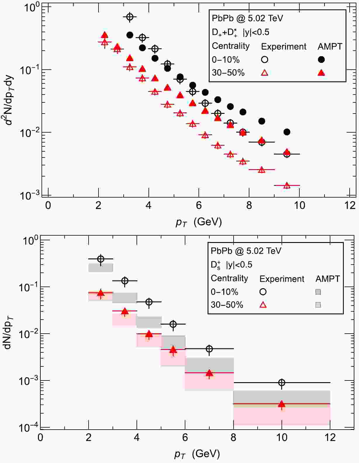
 \sqrt{s_{NN}}= 5.02 TeV by using the framework developed in Ref. [75]. We introduce the production mechanism to produce X_{cs\bar{c}\bar{s}} for its two possible configurations, i.e., the hadronic molecular configurations and the tetraquark configurations into the default version (v1.26t9b) of the AMPT transport model [76]. Given that X_{cs\bar{c}\bar{s}} contains (anti-)charm quarks and (anti-)strange quarks, we need to generate a reasonable number of individual charm and strange quarks in the partonic phase. On top of the default version of AMPT, we modify the factor K ([77]) to enhance the initial c and \bar{c} spectra because of a lack of some channels related to initial heavy quarks. The AMPT calculation gives a reasonable (order-of-magnitude) description of the experimental data [78] for the total yield of D^+ + D^{+*} in the low p_T region (see upper panel of Fig. 1). For the strange quarks, an upper limit on the relative production of strange to non-strange quarks in AMPT is set to 0.6 because of the strangeness enhancement effect (see [79]), and our calculations also give a reasonable (order-of-magnitude) description of the experimental data [80] for the yield of D_s^+ mesons (see lower panel of Fig. 1). The main purpose of this work is to distinguish two inner structures of X_{cs\bar{c}\bar{s}} through their significantly different production rates. The difference in D and D_s^+ meson production between our calculation and experimental data should not influence the relative yield between two inner structures and thus cannot change the qualitative results.

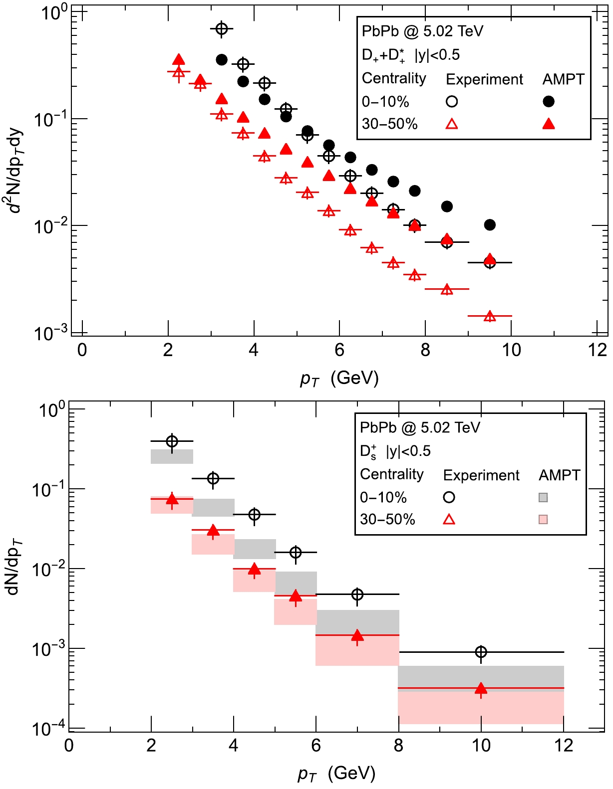
      Figure 1.  (color online) Upper panel: total production of D^+ + D^{+*} from the ALICE Collaboration [78]; lower panel: production of D_s^+ from the ALICE Collaboration [80]. The bands reflect the uncertainty due to the constituent composition, as discussed around Eq. (1), and are obtained by varying the composition fraction by ±10%.

      We use the same production mechanism developed in Ref. [75] for the hadronic molecule and tetraquark configurations of the X_{cs\bar{c}\bar{s}} . For the molecular picture, the charmed-strange mesons are collected after the hadronization process. Then, D_s^+ ( D_s^- ) and D_s^{-*} ( D_s^{+*} ) are coalesced (similar to the hadronization process mentioned in [76]) to form the "molecule" X_{cs\bar{c}\bar{s}} according to the following conditions: the relative distance within the region [5{\rm{fm}},\; 7{\rm{fm}}] and invariant mass within the region [2M_{D_s^+},\; 2M_{D_s^{+*}}] . For the tetraquark picture, the "tetra" X_{cs\bar{c}\bar{s}} is formed via two steps. (i) First, diquarks ( cs ) and diquarks ( \bar{c}\bar{s} ) are formed by matching a (anti-)charm quark with the nearest (in both position space and momentum space) (anti-)strange quark in the parton. (ii) Then, these (anti)diquarks are coalesced to form the X_{cs\bar{c}\bar{s}} according to the following conditions: the relative distance < 1~{\rm{fm}} and invariant mass within the region [2M_{[cs]_1},\; 2M_{[cs]_0}] (the spin triplet and singlet diquark masses are defined in Refs. [30, 31]). Owing to a lack of spin information in the AMPT model for the formation of the charmed-strange mesons and (anti)diquarks, the relative yield ratios are estimated using the thermal model:

      R\left(\frac{A}{B}\right)\equiv \frac{\text{Yield}(A)}{\text{Yield}(B)}= {\rm e}^{-(m_A-m_B)/T_{\text{freezeout}}},

      (1)

      where m_A and m_B represent the masses of hadrons A and B, respectively. Here, T_{\text{freezeout}}\simeq160\; {\rm{MeV}} is the freeze-out temperature. For the hadronic picture, A and B are the D_s^+ and D_s^{+*} mesons, respectively. For the tetraquark picture, A and B are the spin triplet and singlet diquark, respectively. This estimate indicates a composition of 30\% ( 70\% ) for D_s^+ ( D_s^{+*} ) and a composition of 35\% ( 65\% ) for spin triplet(singlet) diquarks. We also vary the composition between 20\% ( 80\% ) and 40\% ( 60\% ) to show the uncertainty bands.

    III.   RESULTS AND DISCUSSIONS
    • Within this simulation framework, we use the Monte Carlo method to generate a total of one million minimum bias events for Pb-Pb collisions at \sqrt{s_{NN}}=5.02\; {\rm{TeV}} . The inclusive yield of X_{cs\bar{c}\bar{s}} is found to be approximately 42000 in the molecular picture and approximately 200 in the tetraquark picture. As a benchmark for comparison, we also estimate the yield of X(3872) within the same framework (see the production mechanism in Ref. [75]; the yield should be multiplied a factor of {1}/{4} owing to wavefunction normalization for both the molecular and tetraquark pictures). The inclusive yield of X(3872) is found to be approximately 171000 in the molecular picture and approximately 600 in the tetraquark picture. The yield of X_{cs\bar{c}\bar{s}} is approximately {1}/{4} of that of X(3872) . Compared with the experimental data of X(3872) measured by the CMS collaboration for PbPb collisions at \sqrt{s_{NN}}=5.02\; {\rm{TeV}} [81], our finding suggests that an observable signal of X_{cs\bar{c}\bar{s}} can be measured in heavy ion collisions at the LHC energy.

      One can also find that the production in the molecular picture significantly exceeds that in the tetraquark picture, by a factor of 200 — a 2-order-of-magnitude difference. This result may be understood as follows: the c-\bar{c} and s-\bar{s} quarks must be pair produced in the initial conditions of heavy ion collisions and then expand and cool with the bulk flow; the molecule X_{cs\bar{c}\bar{s}} needs a large volume to be formed, while the tetraquark X_{cs\bar{c}\bar{s}} needs a compact volume to be formed; thus, the probability of the formation of hadron molecules is far higher than that for the tetraquark state.

      We plot the X_{cs\bar{c}\bar{s}} production as a function of centrality in Pb-Pb collisions at \sqrt{s_{NN}}=5.02\; {\rm{TeV}} for the hadronic molecular state and tetraquark state in Fig. 2. One can find that the yield of the X_{cs\bar{c}\bar{s}} in the molecular picture is 2 orders of magnitude larger than that in the tetraquark picture. From the central collision region to the peripheral collision region, the production first increases then decreases for both the molecular state and the tetraquark state, and the slope of the decrease is far larger in the molecular state than in the tetraquark state. This results from a competing effect between the volume of the bulk system and the size of X_{cs\bar{c}\bar{s}} . For central collisions, the number of (anti-)charm and (anti-)strange quarks is large, the bulk volume is large, and its evolution time is long; thus, the (anti-)charm and (anti-)strange quarks separate sufficiently, which benefits the production of a large-size molecular state. For the peripheral collisions, both the number of (anti-)charm and (anti-)strange quarks and the size of the fireball are small; as such, the evolution time of the fireball is short, which benefits the production of small-sized tetraquark states. This size effect could help to explore the internal structure of X_{cs\bar{c}\bar{s}} through different collision systems, e.g., Pb-Pb, Au-Au, Xe-Xe, Cu-Cu, O-O, and d-A/p-A.

      Figure 2.  (color online) Centrality dependence of the X_{cs\bar{c}\bar{s}} in Pb-Pb collisions at \sqrt{s_{NN}}=5.02\; {\rm{TeV}} for the hadronic molecular configuration (red solid boxes) and tetraquark configuration (blue shaded boxes). The bands reflect both statistical uncertainty from our simulations and the uncertainty due to the constituent composition, as discussed around Eq. (1), and are obtained by varying the composition fraction by ±10%.

      In Fig. 3, we present the rapidity and the transverse momentum distributions of X_{cs\bar{c}\bar{s}} . One can find that the distribution for both the hadronic molecular state and the tetraquark state is similar to that of the usual hadrons [82, 83]. We also show the elliptic flow coefficient v_2 of X_{cs\bar{c}\bar{s}} as a function of the transverse momentum p_T in Fig. 4. The elliptic flow is sensitive to the geometry of the initial fireball and the generation mechanism of X_{cs\bar{c}\bar{s}} .

      Figure 3.  (color online) Rapidity y and transverse momentum p_T distribution of the X_{cs\bar{c}\bar{s}} yield in Pb-Pb collisions at \sqrt{s_{NN}}=5.02\; {\rm{TeV}} for the hadronic molecular configuration (red solid boxes) and the tetraquark configuration (blue shaded boxes). The bands are determined as described in Fig. 2.

      Figure 4.  (color online) Elliptic flow coefficient v_2 versus transverse momentum p_T for the produced X_{cs\bar{c}\bar{s}} in minimum bias Pb-Pb collisions at \sqrt{s_{NN}}=5.02\; {\rm{TeV}} , predicted from our computation for the hadronic molecule picture. The bands are determined as described in Fig. 2.

    IV.   SUMMARY AND OUTLOOK
    • In this work, we studied the yields of X_{cs\bar{c}\bar{s}} for Pb-Pb collisions at \sqrt{s_{NN}}=5.02\;{\rm{TeV}} by introducing the production mechanism of two possible configurations, i.e., the hadronic molecular state and tetraquark state, into the AMPT model. We found that the production in the molecular picture exceeds that in the tetraquark picture by two orders of magnitude. The centrality distribution of the yields of X_{cs\bar{c}\bar{s}} shows a strongly decreasing trend for the hadronic molecular state and a mild change for the tetraquark state. This system size dependence could be a good probe for the inner structure of X_{cs\bar{c}\bar{s}} . We also showed the rapidity and the transverse momentum distributions of X_{cs\bar{c}\bar{s}} production, as well as its elliptic flow coefficient, as a function of the transverse momentum, which can be tested in future experimental measurements. In Ref. [80], a strangeness enhancement effect in heavy ion collisions was found by ALICE collaboration, which could be evidence for quark-gluon plasma. We expect a similar effect to be found in the ratio of X_{cs\bar{c}\bar{s}} to X(3872) , which will be studied in our future work.

    ACKNOWLEDGMENTS
    • The authors would like to thank Dr. J. Liao, E. Wang, Q. Wang, and H. Xing for the helpful discussion.

Reference (83)

目录

/

DownLoad:  Full-Size Img  PowerPoint
Return
Return