


 Abstract
 HTML
HTML Reference
 Related
 PDF
PDF


-
In recent years, the
$ B_{c} $ meson decays have attracted a large amount of research interest for experimental studies [1−8]. Compared with the$ B_{u,d,s} $ mesons, the$ B_{c} $ meson is unique, as it is composed of both heavy quarks with different flavors. It can decay only via weak interaction, because the two flavor asymmetric quarks$ (b $ and$ c) $ cannot be annihilated into gluons (photons) via strong (electromagnetic) interaction. The$ B_{c} $ meson has many rich decay modes, because it has a sufficiently large mass and its constituent quarks (b and c) can decay individually. It provides a very good platform to study the nonleptonic weak decays of heavy mesons, to test the standard model, and to search for new physics signals. With more and more$ B_{c} $ decay events being collected at the Large Hadron Collider (LHC), the$ B_{c} $ meson three-body decays will be an important research topic in both experiment and theory in the next few years.Many approaches based on symmetry principles and factorization theorems have been used to study the
$ B_{(c)} $ meson three-body decays. The former incude the U-spin [9−11], isospin and flavor$ SU(3) $ symmetry [12−14], and factorization assisted topological diagram amplitude approaches [15]. The latter include the QCD-improved factorization approach [16−19] and the PQCD approach [20−30], and it has been proposed that the factorization theorem of three-body B decays is approximately valid when the two particles move collinearly and the bachelor particle recoils back in the final states. According to this quasi-two-body-decay mechanism, the two-hadron distribution amplitudes (DAs) are introduced into the PQCD approach, where the strong dynamics between the two final hadrons in the resonant regions are included.The corresponding two-body decays
$ B_{c}\to D^{*}h $ with$ h=(K^0,\pi^0,\eta,\eta^{\prime}) $ have been studied by the different theories, such as the PQCD approach [31] and the relativistic constituent quark model (RCQM) [32]. In this work, assuming that$ D^{*} $ is an internal resonance state, which further decays into$ D^0\pi^+ $ , we will study the quasi-two-body decays$ B_c\to D^*h\to D^{0}\pi^{+}h $ using the PQCD approach. After the new non-perturbative inputs are introduced, i.e., the two-meson$ D\pi $ distribution amplitudes, the factorization formulas for the$ B_c\to D^*h\to D^{0}\pi^{+}h $ decay amplitudes can be written as [20, 33, 34]$ \begin{array}{*{20}{l}} \mathcal{M}=\Phi_{B_c} \otimes H \otimes \Phi_{D\pi} \otimes \Phi_{h}, \end{array} $

(1) where
$ \Phi_{B_c}(\Phi_{h}) $ denotes the DAs of the initial (final bachelor) meson,$ \Phi_{D\pi} $ is the$ D\pi $ two-meson DAs, and$ \otimes $ denotes the convolution integrations over the parton momenta. Similar to the two-body decay case, the evolution of the hard kernel H for the b quark decay starts with the diagrams of single hard gluon exchange.The remainder of this paper is organized as follows. In Section II, the kinematic variables for the
$ B_{c} $ meson three-body decays are defined. The considered two-meson ($ D\pi $ ) P-wave DAs are parametrized, whose normalization form factors are assumed to follow the relativistic Breit-Wigner (RBW) model. Then, the Feynman diagrams and the total amplitudes for these decays are given. In Section III, the numerical results are presented and discussed. The analytical formulas of the decay amplitudes for each Feynman diagram are presented in the Appendix. -
We begin with the parametrization of the kinematic variables involved in the decays
$ B_c\to D^*h\to D\pi h $ with$ h= (K^0, \pi^0, \eta, \eta^{\prime}) $ . In the rest frame of the$ B_c $ meson, we define the$ B_c $ meson momentum$ P_{B_c} $ , the$ D^* $ meson momentum P, and the bachelor meson h momentum$ P_3 $ in the light-cone coordinates as$ P_{B_c} = \frac{m_{B_c}}{\sqrt{2}}(1,1,0_T), \;\; P = \frac{m_{B_c}}{\sqrt{2}}(1,\eta,0_T), \;\; P_3 = \frac{m_{B_c}}{\sqrt{2}}(0,1-\eta,0_T). $

(2) With the
$ B_c $ meson mass$ m_{B_c} $ . Here,$ \eta = \omega^2/m_{B_c}^2 = s/m_{B_c}^2 $ , with$ \omega^2=s=m^2_{D\pi} $ being the square of the invariant mass of the$ D\pi $ pair. The momenta of the light quarks in the$ B_c $ ,$ D^* $ , and bachelor meson h are denoted as$ k_1 $ ,$ k_2 $ , and$ k_3 $ , respectively:$ \begin{aligned}[b]& k_1 = \left(0,\frac{m_{B_c}}{\sqrt{2}}x_1,k_{1T}\right), \;\;\;\; k_2 = \left(\frac{m_{B_c}}{\sqrt{2}}z,0,k_{2T}\right), \\& k_3 = \left(0,\frac{m_{B_c}}{\sqrt{2}}(1-\eta)x_3,k_{3T}\right), \end{aligned} $

(3) where
$ x_1 $ , z, and$ x_3 $ are the momentum fractions.The P-wave
$ D\pi $ two-meson DAs are defined as in Ref. [35]:$ \Phi_{D \pi}^{P\text{-wave}}=\frac{1}{\sqrt{2 N_{c}}} \not \epsilon_{L} (\not p+\sqrt{s}) \phi_{D \pi}(z, b, s), $

(4) with the distribution amplitude
$ \begin{aligned}[b] \phi_{D \pi}(z, b, s)=&\frac{F_{D \pi}(s)}{2 \sqrt{2 N_{c}}}6 z(1-z)\left[1+a_{D \pi}(1-2 z)\right] \\ &\times\exp \left(-\omega_{D \pi}^{2} b^{2} / 2\right), \end{aligned} $

(5) where the Gegenbauer moment is
$ a_{D\pi} = 0.50 \pm 0.10 $ and the shape parameter is$ \omega_{D\pi} = 0.10 \pm 0.02 $ GeV [35].The strong interactions between the resonance and the final-state meson pair can be factorized into the time-like form factor, which is guaranteed by the Watson theorem [36]. For the narrow resonances, the RBW function [37] is a convenient model for separation from any other resonant or nonresonant contributions with the same spin, and it has been widely used in experimental data analyses. Here, the time-like form factor
$ F_{D\pi}(s) $ can be defined using the matrix element$ \begin{aligned}[b] \langle D(p_1)\pi(p_2)|\bar c\gamma_\mu(1-\gamma_5)q|0\rangle=&\left[(p_1-p_2)_\mu-\frac{m^2_D-m^2_\pi}{p^2}p_\mu\right]\\&\times F_{D\pi}(s) +\frac{m^2_D-m^2_\pi}{p^2}p_\mu F_0(s), \end{aligned} $

(6) where
$ p=p_1+p_2 $ ;$ p_1(p_2) $ and$ m_D(m_\pi) $ represent the$ D(\pi) $ meson momentum and mass, respectively.$ F_{D\pi}(s) $ and$ F_0(s) $ are the P-wave and S-wave form factors, respectively, for the$ D\pi $ system.$ F_{D\pi}(s) $ is parameterized with the RBW line shape$ F_{D \pi}(s)=\frac{\sqrt{s} f_{D^*} g_{D^{*}D \pi}}{m_{D^{*}}^{2}-s- {\rm i} m_{D^{*}} \Gamma(s)}, $

(7) where
$ f_{D^*} $ and$ m_{D^{*}} $ are the decay constant and the pole mass of the$ D^* $ meson, respectively. The coupling constant$ g_{D^{*}D \pi} $ can be determined using the decay width$ \Gamma(s) $ . The invariant mass dependent decay width$ \Gamma(s) $ is defined as$ \Gamma(s)= \Gamma_{0} \Bigg(\frac{q}{q_{0}} \Bigg)^3 \Bigg(\frac{m_{D^{*}}}{\sqrt{s}}\Bigg) {X}^{2}(q r_{\rm BW}), $

(8) where the Blatt-Weisskopf barrier factor is [38]
$ {X}(q r_{\rm BW}) = \sqrt{\frac{1+(q_{0} r_{\rm BW})^{2}}{1+(q r_{\rm BW})^{2}}}, $

(9) with the barrier radius
$r_{\rm BW} = 4.0~\rm GeV^{-1}$ [39, 40]. Here, q represents the momentum for the daughter meson D or π in the$ D^* $ meson rest frame, i.e.,$ q=\frac{1}{2} \sqrt{\left[s-\left(m_{D}+m_{\pi}\right)^{2}\right]\left[s-\left(m_{D}-m_{\pi}\right)^{2}\right] / s}, $

(10) and
$ q_0 $ is the value of q at$ s = m_{D^{*}}^2 $ .The twist-2 distribution amplitude
$ \phi_{h}^{A} $ and the twist-3 ones$ \phi_{h}^{P} $ and$ \phi_{h}^{T} $ have been parameterized as follows [41−43]:$ \begin{aligned}[b] \phi_{h}^{A}(x) =& \frac{f_{h}}{2 \sqrt{2 N_{c}}} 6 x (1-x)\Bigg[1+a_{1}^{h} C_{1}^{3/2} (2 x-1)\\&+a_{2}^{h} C_{2}^{3/2} (2 x-1)+a_{4}^{h} C_{4}^{3/2} (2 x-1) \Bigg], \end{aligned} $

(11) $ \begin{aligned}[b] \phi_{h}^{P}(x) =& \frac{f_{h}}{2 \sqrt{2 N_{c}}} \Bigg[1+\left( 30 \eta_{3}-\frac{5}{2} \rho_{h}^{2} \right) C_{2}^{1/2} (2 x-1)\\&-3 \left( \eta_{3} \omega_{3}+\frac{9}{20} \rho_{h}^{2}(1+6 a_{2}^{h}) \right) C_{4}^{1/2} (2 x-1) \Bigg], \end{aligned} $

(12) $ \begin{aligned}[b] \phi_{h}^{T}(x) =& \frac{f_{h}}{2 \sqrt{2 N_{c}}}(1-2 x)\Bigg[1+6 \Bigg( 5 \eta_{3}-\frac{1}{2} \eta_{3} \omega_{3}\\&-\frac{7}{20} \rho_{h}^{2}-\frac{3}{5}\rho_{h}^{2} a_{2}^{P} \Bigg)(1-10 x+10 x^{2}) \Bigg], \end{aligned} $

(13) where the subscript h represents the pseudoscalar mesons
$ K, \pi $ and the flavor states$\eta_q=\dfrac{u\bar u+d\bar d}{\sqrt2},\; \eta_s=s\bar s$ . Additionally,$\eta_{3}=0.015, \; \omega_{3}=-3$ , and the mass ratios are$\rho_{K(\pi)} = m_{K(\pi)}/m_{0K(\pi)},\;\; \rho_{\eta_q}=2m_q/m_{qq},\;\; \rho_{\eta_s}=2m_s/m_{ss}$ with$m_{0K(\pi)},\; m_{qq}$ , and$ m_{ss} $ being the chiral enhancemnet scales. The Gegenbauer polynomials$ C_{n}^{\nu}(t) $ $ C_{2}^{1/2}(t) = \frac{1}{2}(3 t^{2}-1),\quad C_{4}^{1/2}(t) = \frac{1}{8}(3-30 t^{2}+35 t^{4}), $

(14) $ \begin{aligned}[b]& C_{1}^{3/2}(t) = 3 t, \quad C_{2}^{3/2}(t) = \frac{3}{2}(5 t^{2}-1),\\& C_{4}^{3/2}(t) = \frac{15}{8}(1-14 t^{2}+21 t^{4}). \end{aligned} $

(15) The parameters of the hadronic wave functions are taken from Refs. [44, 45]:
$ \begin{aligned}[b]& a_{1}^{K}=-0.108\pm0.053, \quad a_{2}^{K}=0.170\pm0.046, \\& a_{4}^{K}=0.073\pm0.022, \quad a_{1}^{\pi}=0, \quad a_{2}^{\pi}=0.258\pm0.087, \end{aligned} $

(16) $ \begin{aligned}[b] & a_{4}^{\pi}=0.122\pm0.055,\quad a_{1}^{\eta_{q}}=a_{1}^{\eta_{s}}=0,\\& a_{2}^{\eta_{q}}=a_{2}^{\eta_{s}}=0.115\pm0.115, \quad a_{4}^{\eta_{q}}=a_{4}^{\eta_{s}}=-0.015. \end{aligned} $

(17) For the wave function of the heavy
$ B_c $ meson, we take$ \begin{aligned}[b]& \int {\rm d}^{4} z {\rm e}^{{\rm i} k_{1} \cdot z}\langle 0\left|\bar{b}_{\alpha}(0) c_{\beta}(z)\right| B_{c}\left(P_{B_c}\right)\rangle\\=&\frac{\rm i}{\sqrt{2 N_{c}}}\left[\left(\not P_{B_c}+m_{B_c}\right) \gamma_{5} \phi_{B_{c}}\left(k_{1}\right)\right]_{\beta \alpha}, \end{aligned} $

(18) where we only consider the contribution from the dominant Lorentz structure. In the coordinate space, the distribution amplitude
$ \phi_{B_c} $ with an intrinsic b (the conjugate space coordinate to$ k_T $ ) dependence is adopted in a Gaussian form as [46]$ \phi_{B_{c}}(x, b)=N_{B_{c}} x(1-x) \exp \left[ - \frac{(1-x) m_{c}^{2}+x m_{b}^{2}}{8 \omega_b^{2} x(1-x)} - 2 \omega_b^{2} b^{2} x(1 - x)\right], $

(19) where the shape parameter
$\omega_b = 1.0 \pm 0.1 \;\;\mathrm{GeV}$ is related to the factor$ N_{B_{c}} $ by the normalization$\int_{0}^{1} \phi_{B_{c}}(x, 0) {\rm d} x=1$ . -
For the quasi-two-body decays
$ B_c\to D^*h\to D\pi h $ , the effective Hamiltonian relevant to the$ b\to D (D = d,s) $ transition is given in Ref. [47]:$ \begin{aligned}[b] H_{\rm eff} = &\frac{G_F}{\sqrt{2}}\Bigg[\sum\limits_{q=u,c}V_{qb}V_{qD}^*\{C_1(\mu)O_1^{(q)}(\mu)+C_2(\mu)O_2^{(q)}(\mu)\} \\&-\sum\limits_{i=3\sim10}V_{tb}V_{tD}^*C_i(\mu)O_i(\mu)\Bigg], \end{aligned} $

(20) where the Fermi coupling constant is
$G_F\simeq 1.166\times 10^{-5}~ \rm GeV^{-2}$ [48], and$ V_{qb}V_{qD}^* $ and$ V_{tb}V_{tD}^* $ are the products of the Cabibbo-Kobayashi-Maskawa (CKM) matrix elements. The scale μ separates the effective Hamiltonian into two distinct parts: the Wilson coefficients$ C_i $ and the local four-quark operators$ O_i $ . The local four-quark operators are written as follows:$ \begin{aligned}[b] & O_{1}^{(q)} = \left(\bar{D}_{i} q_{j}\right)_{V-A}\left(\bar{q}_{j} b_{i}\right)_{V-A}, \\ & O_{2}^{(q)} = \left(\bar{D}_{i} q_{i}\right)_{V-A}\left(\bar{q}_{j} b_{j}\right)_{V-A}, \\ & O_{3} = \left(\bar{D}_{i} b_{i}\right)_{V-A} \sum\limits_{q^{\prime}}\left(\bar{q}_{j}^{\prime} q_{j}^{\prime}\right)_{V-A},\\& O_{4} = \left(\bar{D}_{i} b_{j}\right)_{V-A} \sum\limits_{q^{\prime}}\left(\bar{q}_{j}^{\prime} q_{i}^{\prime}\right)_{V-A}, \\ & O_{5} = \left(\bar{D}_{i} b_{i}\right)_{V-A} \sum\limits_{q^{\prime}}\left(\bar{q}_{j}^{\prime} q_{j}^{\prime}\right)_{V+A}, \\ & O_{6} = \left(\bar{D}_{i} b_{j}\right)_{V-A} \sum\limits_{q^{\prime}}\left(\bar{q}_{j}^{\prime} q_{i}^{\prime}\right)_{V+A}, \\& O_{7} = \frac{3}{2}\left(\bar{D}_{i} b_{i}\right)_{V-A} \sum\limits_{q^{\prime}} e_{q^{\prime}}\left(\bar{q}_{j}^{\prime} q_{j}^{\prime}\right)_{V+A},\\ \end{aligned} $

$ \begin{aligned}[b] & O_{8} = \frac{3}{2}\left(\bar{D}_{i} b_{j}\right)_{V-A} \sum\limits_{q^{\prime}} e_{q^{\prime}}\left(\bar{q}_{j}^{\prime} q_{i}^{\prime}\right)_{V+A}, \\ & O_{9} = \frac{3}{2}\left(\bar{D}_{i} b_{i}\right)_{V-A} \sum\limits_{q^{\prime}} e_{q^{\prime}}\left(\bar{q}_{j}^{\prime} q_{j}^{\prime}\right)_{V-A},\\ & O_{10} = \frac{3}{2}\left(\bar{D}_{i} b_{j}\right)_{V-A} \sum\limits_{q^{\prime}} e_{q^{\prime}}\left(\bar{q}_{j}^{\prime} q_{i}^{\prime}\right)_{V-A}, \end{aligned} $

(21) with the color indices i and j. Here
$ V\pm A $ refer to the Lorentz structures$ \gamma_\mu(1\pm \gamma_5) $ .The typical Feynman diagrams at the leading order for the quasi-two-body decays
$ B_c^+\to D^{*+}h\to D^0\pi^+ h $ are shown in Figs. 1 and 2, where we take the decay$ B_c^+\to D^{*+}K^{0} \to D^{0}\pi^{+} K^{0} $ as an example. The analysis formulas for the decay amplitudes of the different Feynman diagrams are given in the appendix.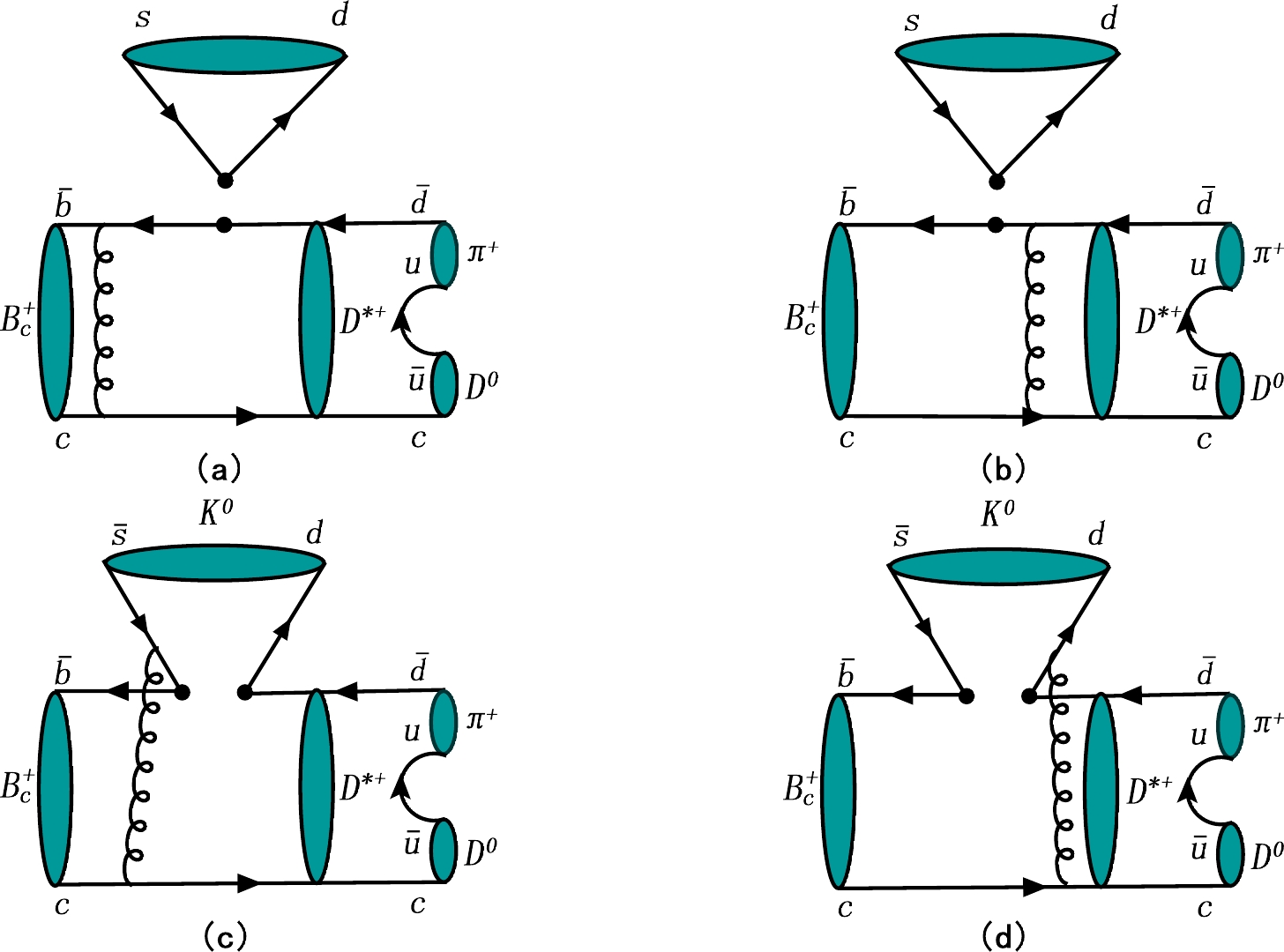
Figure 1. (color online) Factorizable (a)(b) and non-factorizable (c)(d) emission diagrams for the decay
$B_c^+\to D^{*+}K^{0} \to $ $ D^{0}\pi^{+} K^{0}$ .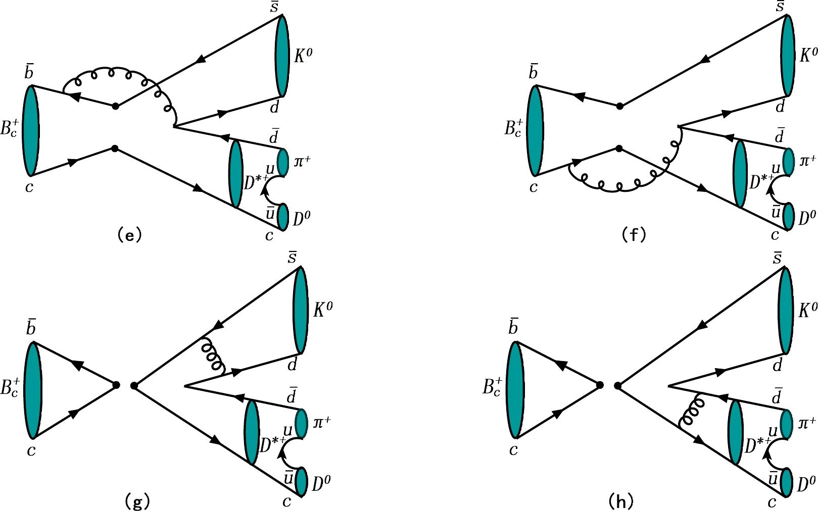
Figure 2. (color online) Nonfactorizable (e)(f) and factorizable (g)(h) annihilation diagrams for the decay
$B_c^+\to D^{*+}K^{0} \to $ $ D^{0}\pi^{+} K^{0}$ .By combining the amplitudes from the different Feynman diagrams, the total decay amplitudes for these considered decays are given as follows:
$ \begin{aligned}[b]& \mathcal{A}\left(B_{c}^+ \rightarrow D^{*+} K^{0}\rightarrow D^0\pi^+K^{0}\right)\\=& V_{cs}V^*_{cb}\left[a_{1} \mathcal{F}_{a}^{L L}+C_{1} \mathcal{M}_{a}^{L L}\right]-V_{ts}V^*_{tb}\left[\left(C_{3}-\frac{1}{2} C_{9}\right) \mathcal{M}_{e}^{L L}\right.\\ &+\left(C_{3}+C_{9}\right) \mathcal{M}_{a}^{L L}+\left(C_{5}-\frac{1}{2} C_{7}\right) \mathcal{M}_{e}^{L R}+\left(C_{5}+C_{7}\right) \mathcal{M}_{a}^{L R} \\ &+\left(C_{4}+\frac{1}{3} C_{3}+C_{10}+\frac{1}{3} C_{9}\right) \mathcal{F}_{a}^{L L}+\left(C_{4}+\frac{1}{3} C_{3}-\frac{1}{2} C_{10}\right.\\ &\left.-\frac{1}{6} C_{9}\right) \mathcal{F}_{e}^{L L}+(C_{6}+\frac{1}{3} C_{5}-\frac{1}{2} C_{8}-\frac{1}{6} C_{7}) \mathcal{F}_{e}^{S P}\\ &\left.+\left(C_{6}+\frac{1}{3} C_{5}+C_{8}+\frac{1}{3} C_{7}\right) \mathcal{F}_{a}^{S P}\right], \end{aligned} $

(22) $ \begin{aligned}[b]& \sqrt{2} \mathcal{A}\left(B_{c}^+ \rightarrow D^{*+} \pi^{0}\rightarrow D^0\pi^+ \pi^{0}\right)\\=& V_{ud}V^*_{ub}\left[a_{2} \mathcal{F}_{e}^{L L}+C_{2} \mathcal{M}_{e}^{L L}\right] -V_{cd}V^*_{cb}\left[a_{1}\mathcal{F}_{a}^{L L}+C_{1} \mathcal{M}_{a}^{L L}\right]\\ &-V_{td}V^*_{tb}\left[\left(\frac{3}{2} C_{10}-C_{3}+\frac{1}{2} C_{9}\right) \mathcal{M}_{e}^{L L}-\left(C_{3}+C_{9}\right) \mathcal{M}_{a}^{L L}\right.\\ &+\left(-C_{5}+\frac{1}{2} C_{7}\right) \mathcal{M}_{e}^{L R}+\left(-C_{4}-\frac{1}{3} C_{3}-C_{10}-\frac{1}{3} C_{9}\right) \mathcal{F}_{a}^{L L}\\ &+\left(C_{10}+\frac{5}{3} C_{9}-\frac{1}{3} C_{3}-C_{4}-\frac{3}{2} C_{7}-\frac{1}{2} C_{8}\right) \mathcal{F}_{e}^{L L} \\ &+\left(-C_{6}-\frac{1}{3} C_{5}+\frac{1}{2} C_{8}+\frac{1}{6} C_{7}\right) \mathcal{F}_{e}^{S P}-\left(C_{5}+C_{7}\right) \mathcal{M}_{a}^{L R} \\ &\left.+\left(-C_{6}-\frac{1}{3} C_{5}-C_{8}-\frac{1}{3} C_{7}\right) \mathcal{F}_{a}^{S P}\right], \end{aligned} $

(23) $ \begin{aligned}[b]& \sqrt{2} \mathcal{A}\left(B_{c}^+ \rightarrow D^{*+} \eta_{q}\rightarrow D^0\pi^+ \eta_{q}\right)\\= &V_{ud}V^*_{ub}\left[a_{2} \mathcal{F}_{e}^{L L}+C_{2} \mathcal{M}_{e}^{L L}\right]+V_{cd}V^*_{cb}\left[a_{1} \mathcal{F}_{a}^{L L}+C_{1} \mathcal{M}_{a}^{L L}\right] \\ & -V_{td}V^*_{tb}\left[\left(2 C_{4}+C_{3}+\frac{1}{2} C_{10}-\frac{1}{2} C_{9}\right) \mathcal{M}_{e}^{L L}+\left(C_{3}+C_{9}\right) \mathcal{M}_{a}^{L L}\right. \\ & +\left(C_{5}-\frac{1}{2} C_{7}\right) \mathcal{M}_{e}^{L R}+\left(C_{5}+C_{7}\right) \mathcal{M}_{a}^{L R}+\left(C_{4}+\frac{1}{3} C_{3}+C_{10}\right. \\ & \left.+\frac{1}{3} C_{9}\right) \mathcal{F}_{a}^{L L}+\left(\frac{7}{3} C_{3}+\frac{5}{3} C_{4}+\frac{1}{3}\left(C_{9}-C_{10}\right)\right) \mathcal{F}_{e}^{L L}+\left(2 C_{5}\right. \\ & \left.+\frac{2}{3} C_{6}+\frac{1}{2} C_{7}+\frac{1}{6} C_{8}\right) \mathcal{F}_{e}^{L R}+\left(C_{6}+\frac{1}{3} C_{5}-\frac{1}{2} C_{8}-\frac{1}{6} C_{7}\right) \mathcal{F}_{e}^{S P} \\ & \left.+\left(C_{6}+\frac{1}{3} C_{5}+C_{8}+\frac{1}{3} C_{7}\right) \mathcal{F}_{a}^{S P}\right], \end{aligned} $

(24) $ \begin{aligned}[b]& \mathcal{A}\left(B_{c}^+ \rightarrow D^{*+} \eta_{s}\rightarrow D^0\pi^+ \eta_{s}\right) \\= & -V_{td}V^*_{tb}\left[\left(C_{4}-\frac{1}{2} C_{10}\right) \mathcal{M}_{e}^{L L}+\left(C_{6}-\frac{1}{2} C_{8}\right) \mathcal{M}_{e}^{S P}+\left(C_{3}+\frac{1}{3} C_{4}\right.\right. \\ & \left.\left.-\frac{1}{2} C_{9}-\frac{1}{6} C_{10}\right) \mathcal{F}_{e}^{L L}+\left(C_{5}+\frac{1}{3} C_{6}-\frac{1}{2} C_{7}-\frac{1}{6} C_{8}\right) \mathcal{F}_{e}^{L R}\right], \end{aligned} $

(25) where the combinations of the Wilson coefficients are
$ a_{1}=C_{2}+C_{1} / 3 $ and$ a_{2}=C_{1}+C_{2} / 3 $ .It should be noticed that Eqs. (24) and (25) give the decay amplitudes corresponding to the flavor states
$ \eta_{q} $ and$ \eta_{s} $ , respectively. For the physical states$ (\eta, \eta^{\prime}) $ , the decay amplitudes are written as follows:$ \begin{aligned}[b]& \mathcal{A}\left(B_{c}^+ \rightarrow D^{*+} \eta\rightarrow D^0\pi^+ \eta\right) \\=& \mathcal{A}\left(B_{c}^+ \rightarrow D^{*+} \eta_{q}\rightarrow D^0\pi^+ \eta_{q}\right) \cos \phi\\&-\mathcal{A}\left(B_{c}^+ \rightarrow D^{*+} \eta_{s}\rightarrow D^0\pi^+ \eta_{s}\right) \sin \phi, \end{aligned} $

(26) $ \begin{aligned}[b]& \mathcal{A}\left(B_{c}^+ \rightarrow D^{*+} \eta^{\prime}\rightarrow D^0\pi^+ \eta^{\prime}\right) \\=& \mathcal{A}\left(B_{c}^+ \rightarrow D^{*+} \eta_{q}\rightarrow D^0\pi^+ \eta_{q}\right) \sin \phi\\&+\mathcal{A}\left(B_{c}^+ \rightarrow D^{*+} \eta_{s}\rightarrow D^0\pi^+ \eta_{s}\right) \cos \phi, \end{aligned} $

(27) where
$ \phi=39.3^{\circ}\pm1.0^\circ $ [49] is the mixing angle between these two flavor states, and the physical states are defined as follows:$ \begin{array}{*{20}{l}} \left(\begin{array}{c} \eta \\ \eta^{\prime} \end{array}\right) & = \left(\begin{array}{cc} \cos \phi & -\sin \phi \\ \sin \phi & \cos \phi \end{array}\right)\left(\begin{array}{l} \eta_{q} \\ \eta_{s} \end{array}\right). \end{array} $

(28) Then, the differential decay rate is described as [50, 51]
$ \frac{{\rm d} \mathcal{B}}{{\rm d} s}=\frac{\tau_{B_c} q^{3} q^{3}_{h}}{48 \pi^{3} m_{B_c}^{7}} \overline{|{\mathcal{A}}|^{2}}, $

(29) where
$ \tau_{B_c} $ represents the$ B_c $ meson mean lifetime, and the kinematic variable$ q_h $ denotes the momentum magnitude of the bachelor meson h in the center-of-mass frame of the$ D\pi $ pair:$ q_{h}=\frac{1}{2}\sqrt{[(m_{B_c}^2-m_h^2)^2-2(m_{B_c}^2+m_h^2)s+s^2]/s}. $

(30) -
The input parameters adopted in our numerical calculations are summarized as follows (the masses, decay constants, and QCD scale are in units of GeV, and the
$ B_c $ meson lifetime is in units of ps) [31, 43, 48]:$ \begin{aligned}[b] \Lambda^{(5)}_{\rm QCD} =& 0.112,\;\;\; m_{B_c^+} = 6.27447,\;\;\; m_b = 4.18,\;\\ m_{K^0} =& 0.498,\;\;\; m_{0K} = 1.7,\;\;\; m_{\pi^{\pm}} = 0.140, \end{aligned} $

(31) $ \begin{aligned}[b] m_{\pi^0}=& 0.135,\;\;\; m_{0\pi}= 1.3,\;\;\;m_\eta=0.548,\;\\ m_{\eta^\prime}=&0.958,\;\;\; m_{qq}=0.110, \;\;\;m_{ss}=0.707, \end{aligned} $

(32) $ \begin{aligned}[b] m_{D^{*\pm}} =& 2.010,\;\;\;m_{D^{0}}=1.865,\;\;\;\tau_{B_{c}^+}= 0.510,\;\\ f_{B_c} =& 0.489,\;\;\; f_{D^*} = 0.25,\;\;\;f_{K} = 0.16, \end{aligned} $

(33) $ f_{\pi} = 0.13,\;\;f_{\eta_{q}}=(1.07\pm0.02)f_{\pi},\;\; f_{\eta_{s}} = (1.34\pm0.06)f_{\pi}. $

(34) For the CKM matrix elements, we employ the Wolfenstein parametrization with the inputs [48]
$ \lambda=0.22453 \pm 0.00044, \quad A=0.836 \pm 0.015, $

(35) $ \bar{\rho}=0.122_{-0.017}^{+0.018}, \quad \bar{\eta}=0.355_{-0.011}^{+0.012}. $

(36) Using the decay amplitudes given in the Appendix, the total amplitudes given by Eqs. (23)–(27), and the differential branching ratio given by Eq. (29), by integrating over the full
$ D\pi $ invariant mass region$ (m_D + m_{\pi})\leq \sqrt{s}\leq (m_{B_c}-m_h)^2 $ with$ h=(K^0, \pi^0, \eta^{(\prime)}) $ , we obtain the branching ratios for the quasi-two-body decays:$ \begin{aligned}[b]& {\rm Br}\left(B_{c}^+ \to D^{*+} K^{0}\rightarrow D^0\pi^+K^{0}\right) \\=& \left({5.22}_{-0.38-0.45-0.00-0.21-0.15-0.37}^{+0.53+0.47+0.21+0.09+0.15+0.41}\right)\times{10}^{-6}, \end{aligned} $

(37) $ \begin{aligned}[b]& {\rm Br}\left(B_{c}^+ \rightarrow D^{*+} \pi^{0}\rightarrow D^0\pi^+ \pi^{0} \right) \\=& \left({0.93}_{-0.08-0.08-0.23-0.03-0.02-0.05}^{+0.11+0.09+0.21+0.01+0.03+0.06}\right)\times{10}^{-7}, \end{aligned} $

(38) $ \begin{aligned}[b]& {\rm Br}\left(B_{c}^+ \rightarrow D^{*+} \eta\rightarrow D^0\pi^+\eta \right) \\=& \left({2.83}_{-0.19-0.23-0.21-0.25-0.20-0.18}^{+0.22+0.25+0.19+0.28+0.18+0.31}\right)\times{10}^{-8}, \end{aligned} $

(39) $ \begin{aligned}[b]& {\rm Br} (B_{c}^+ \rightarrow D^{*+} \eta^{\prime}\rightarrow D^0\pi^+\eta^{\prime} ) \\=& \left({1.89}_{-0.12-0.16-0.14-0.15-0.16-0.15}^{+0.13+0.17+0.12+0.19+0.14+0.21}\right)\times{10}^{-8}, \end{aligned} $

(40) where the first error originates from the shape parameter in the
$ B_c $ meson DAs, i.e.,$ \omega_{B_c}=1.0\pm0.1 $ GeV; the second error comes from the decay constant$ f_{D^{*}}=(250\pm 11) $ MeV; the third and the fourth errors are induced by the Gegenbauer coefficient$ a_{D\pi}=0.50\pm0.10 $ and the shape parameter$ \omega_{D\pi}=0.10\pm0.02 $ GeV in the$ D\pi $ pair DAs, respectively; the fifth error is caused by the decay width of the resonance$ D^{*+} $ , i.e.,$ \Gamma_{D^{*+}}=83.3\pm2.6 $ keV; and the last error is induced by the next-to-leading-order effect in the PQCD approach, where the hard scale t is changed from 0.75t to 1.25t. Other errors, which come from the uncertainties of the parameters in the DAs of the bachelor meson h, the Wolfenstein parameters, etc., have been neglected because they are very small.If we assume the isospin conservation for the strong decay
$ D^*\to D\pi $ ,$ \frac{\Gamma(D^{*+}\to D^0\pi^+)}{\Gamma(D^{*+}\to D\pi)}=2/3. $

(41) Under the narrow width approximation relation, the branching ratios of these quasi-two-body decays can be written as
$ \begin{aligned}[b]& {\rm Br}\left(B_{c}^+\to D^{*+} h \to D^0\pi^+ h \right) \\=& {\rm Br} (B_{c}^+\to D^{*+}h)\cdot {\rm Br} (D^{*+}\to D^0\pi^+). \end{aligned} $

(42) According to Eqs. (41) and (42), we can obtain the branching ratios of the corresponding two-body decays:
$ {\rm Br}(B_{c}^+\to D^{*+}K^0) = \left({7.83}_{-0.57-0.67-0.00-0.31-0.23-0.55}^{+0.79+0.70+0.32+0.13+0.22+0.61}\right)\times{10}^{-6}, $

(43) $ {\rm Br}(B_{c}^+\to D^{*+}\pi^0) = \left({1.40}_{-0.12-0.12-0.35-0.05-0.03-0.07}^{+0.16+0.13+0.32+0.01+0.04+0.09}\right)\times{10}^{-7}, $

(44) $ {\rm Br}(B_{c}^+\to D^{*+}\eta) = \left({4.25}_{-0.29-0.35-0.32-0.38-0.30-0.27}^{+0.33+0.38+0.29+0.42+0.27+0.47}\right)\times{10}^{-8}, $

(45) $ {\rm Br}(B_{c}^+\to D^{*+} \eta^{\prime}) =\left({2.84}_{-0.18-0.24-0.21-0.23-0.24-0.23}^{+0.20+0.26+0.18+0.29+0.21+0.32}\right)\times{10}^{-8}, $

(46) where we assume the branching ratio of the decay
$ D^{*+}\to D\pi $ to be$ 100\% $ , assume isospin conservation, and use the narrow width approximation.The branching ratios of the two-body decays
$ B_c\to D^*h $ with$ h= (K^0, \pi^0, \eta, \eta^{\prime}) $ have been calculated in the PQCD approach [31], where the results were given as$ {\rm Br}(B_{c}^+\to D^{*+}K^0) = \left({7.78}_{-2.40-0.02-0.52}^{+2.54+0.02+0.72}\right)\times{10}^{-6}, $

(47) $ {\rm Br}(B_{c}^+\to D^{*+}\pi^0) = \left({1.3}_{-0.3-0.3-0.0}^{+0.4+0.2+0.0}\right)\times{10}^{-7}, $

(48) $ {\rm Br}(B_{c}^+\to D^{*+}\eta) = \left({3.4}_{-0.9-1.5-0.00}^{+1.4+1.9+0.4}\right)\times{10}^{-8}, $

(49) $ {\rm Br}(B_{c}^+\to D^{*+} \eta^{\prime}) =\left({1.5}_{-0.5-0.6-0.1}^{+0.8+0.8+0.3}\right)\times{10}^{-8}. $

(50) From the upper formulas, one can find that the branching ratios of the decays
$ B_{c}^+\to D^{*+}h $ calculated in two-body and three-body frameworks are consistent with each other within errors. The decay widths for the decays$ B_{c}^+\to D^{*+}K^0 $ and$ B_{c}^+\to D^{*+}\pi^0 $ were calculated by using the RCQM [32] and are given as$ \Gamma(B_{c}^+\to D^{*+}K^0)= 4.10\times10^{-19} $ GeV and$ \Gamma(B_{c}^+\to D^{*+}\pi^0)=9.83\times10^{-20} $ GeV, respectively. Taking$ \tau_{B_{c}^+}= 0.510 $ ps, we can obtain their branching ratios as${\rm BR} (B_{c}^+\to D^{*+}K^0)=3.18\times10^{-7}$ and${\rm Br}(B_{c}^+\to D^{*+}\pi^0)=0.76\times10^{-7}$ , respectively, which are far smaller than the PQCD predictions. From Eqs. (22) and (23), one can find that the dominant contributions for these two decays come from the factorization annihilation amplitude$ \mathcal{F}_{a}^{L L} $ asociated with the large Wilson coefficient$ a_1 $ . Unfortunately, this type of annihilation contribution is not calculable under the RCQM. We hope that it can be verified by future experiments. As we know, the annihilation diagram contributions associated with the CKM matrix elements$ V^*_{cb}V_{cs} $ are dominant in both the decays$ B^+_c\to D^{*0}K^+ $ and$ B^+_c\to D^{*+}K^0 $ . In fact, such contributions are the same for these two channels; thus, we argue that the branching ratios for these two decays$ B^+_c\to D^{*0}K^+ $ and$ B^+_c\to D^{*+}K^0 $ should be close to each other. For example,${\rm Br}(B^+_c\to D^{*0}K^+)=(7.35^{+3.28}_{-2.34})\times10^{-6}$ and${\rm Br}(B^+_c\to D^{*+}K^0)=(7.78^{+2.64}_{-2.46})\times10^{-6}$ were given by the PQCD approach [31]. In Ref. [52], the upper limit for$ R_{D^{*0}K^+} $ at the$ 95\% $ confidence level was given as$ R_{D^{*0}K^+}=\frac{f_c}{f_u}{\rm Br}(B^+_c\to D^{*0}K^+)<1.1\times 10^{-6}, $

(51) where
$ f_c/f_u $ is the ratio of the inclusive production cross-sections of$ B^+_c $ and$ B^+ $ mesons, which can be related to the decays$ B^+_c\to J/\Psi\pi^+ $ and$ B^+\to J/\Psi K^+ $ through the formula$ R_{c/u}=\frac{f_c}{f_u}\frac{{\rm Br}(B^+_c\to J/\Psi \pi^+)}{{\rm Br}(B^+\to J/\Psi K^+)}, $

(52) and it was measured as
$ R_{c/u}=(0.68\pm0.10)\% $ by the LHCb collaboration [9]. Unfortunately,${\rm Br}(B^+_c\to J/\Psi\pi^+)$ has not been well measured via experiments. According to different theoretical predictions, the LHCb collaboration gave a range of$ 0.004\sim0.012 $ for the$ f_c/f_u $ values [52]. Then, we can obtain the lowest upper limit for the branching ratio of the decay$ B^+_c\to D^{*0}K^+ $ $ \begin{array}{*{20}{l}} {\rm Br}(B^+_c\to D^{*0}K^+)<9.2\times 10^{-5}. \end{array} $

(53) Certainly, the upper limit here is strongly dependent on the branching ratio of the decay
$ B^+_c\to J/\Psi\pi^+ $ . As a rough estimate, this upper limit can also be applied to the branching ratio of the decay$ B^+_c\to D^{*+}K^0 $ . Our prediction is found to satisfy this limit, which can be tested by the present LHCb experiments. There exists constructive (destrutive) interference between the amplitudes$ \mathcal{A}\left(B_{c}^+ \to D^{*+} \eta_{q}\to D^0\pi^+ \eta_{q}\right) $ and$ \mathcal{A} (B_{c}^+\to D^{*+} \eta_{s}\to D^0\pi^+ \eta_{s}) $ in the decay$ B_{c}^+\to D^{*+}\eta\to D^0\pi^+ \eta (B_{c}^+\to D^{*+}\eta^\prime\to D^0\pi^+ \eta^\prime) $ , which increases (reduces) the branching ratio of the corresponding decay.Last, we discuss the invariant mass
$ m_{D\pi} $ -dependence of the decay spectrum. Here, we take the decay$ B_{c}^+ \to D^{*+} \pi^{0}\to D^0\pi^+ \pi^{0} $ as an example and plot the$ m_{D\pi} $ -dependence of the differential branching fraction in Fig. 3, where a maximum in the$ D\pi $ pair invariant mass is observed at approximately 2.010 GeV. It is easy to see that the main contribution to the branching ratio comes from the region around the pole mass of the$ D^{*+} $ resonance, as we expected. The peak located at the$ D^{*+} $ mass is very sharp, because the decay width is tiny, i.e.,$ \Gamma_{D^{*+}}=83.3 $ keV [53, 54]; at the same time, the$ D^0\pi^+ $ threshold is too close to the resonance mass$ m_{D^{*+}} $ . This differs significantly from the case of the$ K^{*} $ resonance [22], whose mass is far larger than the$ K\pi $ threshold. If we integrate over$ m_{D\pi} $ by limiting the range of$ m_{D\pi}=[m_{D^{*+}}-\delta_m,m_{D^{*+}}+\delta_m] $ with$ \delta_m=2\Gamma_{D^{*+}}, 3\Gamma_{D^{*+}}, 4\Gamma_{D^{*+}} $ , we can find that the corresponding branching factions are$93.6\%, ~94.3\%,~ 95.0\%$ of the total branching ratio${\rm Br}(B_{c}^+ \rightarrow D^{*+} \pi^{0}\rightarrow D^0\pi^+ \pi^{0})= 0.93\times10^{-7}$ . In contrast, if we consider the virtual contribution from the region$ 2.1\sim3.5 $ GeV of the invariant mass$ m_{D\pi} $ shown in the right panel of Fig. 3, the corresponding branching fraction only amounts to$ 7.1\% $ of the total. The situation is simliar for the other decay channels.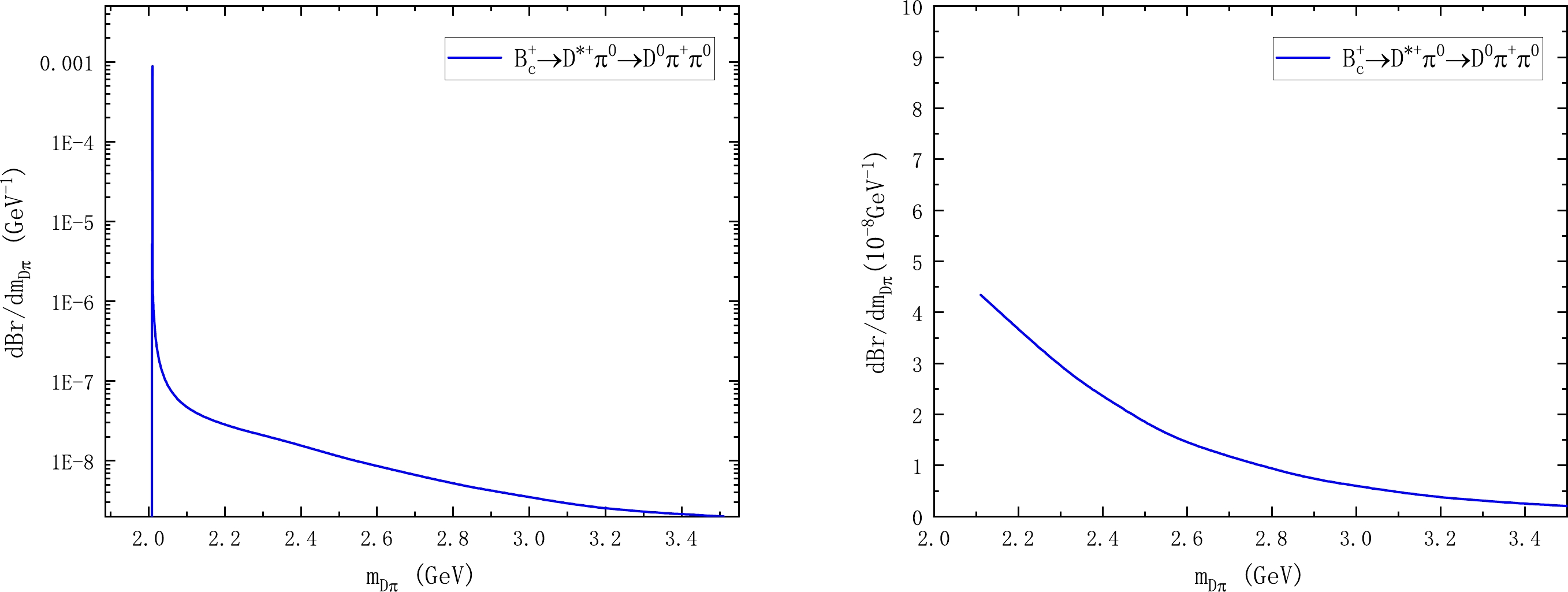
Figure 3. (color online) Invariant mass
$ m_{D\pi} $ dependence of the differential branching fraction for the decay$ B_c\to D^{*+}\pi^{0}\to D^{0}\pi^{+} \pi^{0} $ (left panel) and the corresponding virtual contribution in the$ m_{D\pi} $ region$ 2.1\sim3.5 $ GeV (right panel). -
In this paper, we studied the quasi-two-body decays
$ B_{c}^+\to D^{*+}h\to D^0\pi^+ h $ with$ h=(K^0,\pi^0,\eta^{(\prime)}) $ in the PQCD approach. The di-meson distribution amplitude for the$ D\pi $ system with the P-wave time-like form factor$ F_{D\pi}(s) $ is employed to describe the$ D^{*+} $ resonance and its interactions with the$ D^0\pi^+ $ pair. We predict the branching ratios of the concerned decays and find the following:1. The branching ratios of the quasi-two-body decays
$ B_{c}^+\to D^{*+}h\to D^0\pi^+ h $ exhibit an obvious hierarchy$ \begin{aligned}[b]& {\rm Br}(B_{c}^+\to D^{*+}K^0\to D^0\pi^+ K^0)\\&> {\rm Br}(B_{c}^+\to D^{*+}\pi^0\to D^0\pi^+ \pi^0)\\&> {\rm Br}(B_{c}^+\to D^{*+}K^0\to D^0\pi^+ \eta^{(\prime)}), \end{aligned} $

(54) where
${\rm Br}(B_{c}^+\to D^{*+}K^0\to D^0\pi^+ K^0)$ is the largest one and reaches the order of$ 10^{-6} $ . Thus, the decay$ B_{c}^+\to D^{*+}K^0\to D^0\pi^+ K^0 $ can be observed by future LHCb experiments.2. Using the narrow width approximation relation and the isospin conservation
$ \Gamma(D^{*+}\to D^0\pi^+)/\Gamma(D^{*+}\to D\pi)= 2/3 $ , we can relate the branching ratios of these quasi-two-body decays$ B_{c}^+\to D^{*+}h\to D^0\pi^+ h $ with those of the corresponding two-body channels$ B_{c}^+\to D^{*+}h $ . Our results for the branching ratios of the decays$ B_{c}^+\to D^{*+}h $ are consistent with the previous PQCD calculations within errors, while there is considerable tension between the predictions of the PQCD approach and the RCQM for the decay$ B_{c}^+\to D^{*+}K^0 $ . The former is one order of magnitude larger than the latter. This is because the annihilation type contribution is dominant for the decay$ B_{c}^+\to D^{*+}K^0 $ , which is not calculable under the RCQM.3. The branching ratio of the decay
$ B_{c}^+\to D^{*+}\eta\to D^{0}\pi^+\eta $ is larger than that of$ B_{c}^+\to D^{*+}\eta^\prime\to D^{0}\pi^+\eta^\prime $ , which is induced by the opposite interferences between the amplitudes$ \mathcal{A}\left(B_{c}^+ \rightarrow D^{*+} \eta_{q}\rightarrow D^0\pi^+ \eta_{q}\right) $ and$ \mathcal{A} (B_{c}^+\to D^{*+} \eta_{s}\to D^0\pi^+ \eta_{s}) $ .4. From the
$ D^0\pi^+ $ invariant mass$ m_{D^0\pi^+} $ -dependences of these concerned decay spectrums, one can find that the main portions of the branching fractions are concentrated in a very small region of the$ m_{D^0\pi^+} $ . For example, approximately$ 94\% $ of the branching ratio of the decay$ B_{c}^+\to D^{*+}\pi^0\to D^{0}\pi^+\pi^0 $ comes from the realm of$ 2.1 $ MeV around the$ D^{*+} $ pole mass. -
In this appendix, we present the PQCD factorization formulas for the amplitudes of the decays
$ B\to D^{*+}h\to D^0\pi^+ h $ $ \begin{aligned}[b] \mathcal{F}_{e}^{LL} =&4 \sqrt{2}G_F C_F \pi f_h (\eta -1) m_{B_c}^4 \int_0^1 {\rm d} x_1 {\rm d} z\int_0^{\infty}b_1{\rm d}b_1b_2{\rm d}b_2\phi_{B_c}(x_1,b_1)\phi_{D \pi}(z,b_2,\omega)\Big\{ [\sqrt{\eta } (r_b+2 z-2)\\{} &-2 r_b-z+1]h(\alpha_e,\beta_a,b_1,b_2)E_a(t_a)-\eta h(\alpha_e,\beta_b,b_2,b_1)E_b(t_b)\Big\}, \end{aligned}\tag{A1} $ 
$ \begin{aligned}[b] \mathcal{F}_{e}^{SP} =&-8 \sqrt{2} G_F C_F \pi f_h r_h m_{B_c}^4 \int_0^1{\rm d}x_1{\rm d}z\int_0^{\infty}b_1{\rm d}b_1b_2{\rm d}b_2\phi_B(x_1,b_1)\phi_{D \pi}(z,b_2,\omega)\Big\{[(\eta-1)rb-\sqrt{\eta}z+2 \eta(z-1) \\{} &+2]h(\alpha_e,\beta_a,b_1,b_2)E_a(t_a)+x_1h(\alpha_e,\beta_b,b_2,b_1)E_b(t_b)\Big\}, \end{aligned}\tag{A2} $

$ \begin{aligned}[b] \mathcal{M}_{e}^{LL} =&16 \frac{\sqrt{3}}{3} G_F C_F \pi (\eta -1) m_{B_c}^4\int_0^1{\rm d}x_1{\rm d}z{\rm d}x_3\int_0^{\infty}b_1{\rm d}b_1b_3{\rm d}b_3\phi_{B_c}(x_1,b_1)\phi_{D \pi}(z,b_1,\omega)\phi_h^{A}(x_3)(x_3)\Big\{ (\eta -x_1- \eta x_3 \\{} &+x_3+ \eta z - \sqrt{\eta} z -1)h(\beta_c,\alpha_e,b_1,b_3)E_{cd}(t_c) -(x_1+\eta x_3-x_3+\sqrt{\eta } z-z)h(\beta_d,\alpha_e,b_1,b_3)E_{cd}(t_d)\Big\}, \end{aligned}\tag{A3} $

$ \begin{aligned}[b] \mathcal{M}_{e}^{LR} =&-16 \frac{\sqrt{3}}{3} G_F C_F \pi r_h (\sqrt{\eta} -1) m_{B_c}^4\int_0^1{\rm d}x_1{\rm d}z{\rm d}x_3\int_0^{\infty}b_1{\rm d}b_1b_3{\rm d}b_3\phi_{B_c}(x_1,b_1)\phi_{D \pi}(z,b_1,\omega)\Big\{[\phi_h^{P}(x_3) (\eta +x_1\\{} &-\eta x_3+x_3-\sqrt{\eta } z-1)+\phi_h^{T}(x_3) \left(\eta +x_1-\eta x_3+x_3+\sqrt{\eta } z-1\right)]h(\beta_c,\alpha_e,b_1,b_3)E_{cd}(t_c)\\{} &-[x_1 (\phi_h^{P}(x_3)-\phi_h^{T}(x_3))+(\eta -1) x_3 (\phi_h^{P}(x_3)-\phi_h^{T}(x_3))-\sqrt{\eta } z (\phi_h^{P}(x_3)+\phi_h^{T}(x_3))]\\{} &\times h(\beta_d,\alpha_e,b_1,b_3)E_{cd}(t_d)\Big\}, \end{aligned}\tag{A4} $

$ \begin{aligned}[b] \mathcal{M}_{e}^{SP} =&-16 \frac{\sqrt{3}}{3} G_F C_F \pi (\eta-1) m_{B_c}^4 \int_0^1 {\rm d}x_1{\rm d}z{\rm d}x_3 \int_0^{\infty}b_1{\rm d}b_1b_3{\rm d}b_3\phi_{B_c}(x_1,b_1)\phi_{D \pi}(z,b_1, \omega) \Big\{[(\eta+x_1-\eta x_3+x_3 \\{} &+\eta z-\sqrt{\eta} z-1) \phi_{h}^{A}(x_3)]h(\beta_c,\alpha_e,b_1,b_3)E_{ef}(t_e)-[(x_1+\eta x_3-x_3+\sqrt{\eta}z-z) \phi_{h}^{A}(x_3)]\\{} &\times h(\beta_d,\alpha_e,b_1,b_3)E_{ef}(t_f)\Big\}, \end{aligned}\tag{A5} $

$ \begin{aligned}[b] \mathcal{M}_{a}^{LL} =&16 \frac{\sqrt{3}}{3} G_F C_F \pi m_{B_c}^4\int_0^1{\rm d}x_1{\rm d}z{\rm d}x_3\int_0^{\infty}b_1{\rm d}b_1b_2{\rm d}b_2\phi_{B_c}(x_1,b_1)\phi_{D \pi}(z,b_2,\omega)\Big\{[(\eta -1) \phi_h^{A}(x_3) (\eta +r_b\\{} &-\eta x_3+x_3+\eta z -1)+\sqrt{\eta } r_h (\phi_h^{T}(x_3) (-\eta +(\eta-1) x_3+ z+1)+\phi_h^{P}(x_3) (\eta -\eta x_3+x_3+z-1))] \\{} &h(\beta_e,\alpha_a,b_1,b_2)E_{ef}(t_e)-[(\eta -1) \phi_h^{A}(x_3) (r_c+(\eta -1) (z-1))+\sqrt{\eta } r_h (\phi_h^{P}(x_3) (\eta -x_1-\eta x_3+x_3+z-1)\\{} &+\phi_h^{T}(x_3) (x_1+\eta (x_3-1)-x_3+z-1))]h(\beta_f,\alpha_a,b_1,b_2)E_{ef}(t_f)\Big\}, \end{aligned}\tag{A6} $

$ \begin{aligned}[b] \mathcal{M}_{a}^{LR} =&-16 \frac{\sqrt{3}}{3} G_F C_F \pi m_{B_c}^4\int_0^1{\rm d}x_1{\rm d}z{\rm d}x_3\int_0^{\infty}b_1{\rm d}b_1b_2{\rm d}b_2\phi_{B_c}(x_1,b_1)\phi_{D \pi}(z,b_2,\omega)\Big\{[(\eta -1) r_b (\sqrt{\eta } \phi_h^{A}(x_3)\\{} &-r_h \phi_h^{P}(x_3)) +(\eta+1) r_b r_h \phi_h^{T}(x_3)+(\eta-1) r_P (x_3-1) (\phi_h^{P}(x_3)+\phi_h^{T}(x_3))+z (\eta^{3/2} \phi_h^{A}(x_3)-\sqrt{\eta} \phi_h^{P}(x_3)\\{} &+\eta r_h (\phi_h^{T}(x_3)-\Phi_h^{P}(x_3)))]h(\beta_e,\alpha_a,b_1,b_2)E_{ef}(t_e) -[r_h (\phi_h^{P}(x_3)+\phi_h^{T}(x_3)) (r_c+x_1-x_3)\\{} &+\eta^{3/2} \phi_h^{A}(x_3) (r_c+z-1)-\sqrt{\eta} \phi_h^{A}(x_3) (r_c+z-1) ]h(\beta_f,\alpha_a,b_1,b_2)E_{ef}(t_f)\Big\}, \end{aligned}\tag{A7} $

$ \begin{aligned}[b] \mathcal{F}_{a}^{LL} =&-4 \sqrt{2}G_F C_F \pi f_{B_c} m_{B_c}^4 \int_0^1{\rm d}z{\rm d}x_3\int_0^{\infty}b_2{\rm d}b_2b_3{\rm d}b_3\phi_{D \pi}(z,b_2,\omega)\Big\{[(\eta -1) (z-1) \phi_h^{A}(x_3)\\{} &-2 \sqrt{\eta } r_h z \phi_h^{P}(x_3)]h(\alpha_a,\beta_g,b_2,b_3)E_{g}(t_g)-[-(\eta -1) (\eta \phi_h^{A}(x_3)+r_c r_h \phi_h^{P}(x_3))-(\eta +1) r_c r_h \phi_h^{T}(x_3)\\{} &+(\eta-1)^{2} x_3 \phi_h^{A}(x_3))]h(\alpha_a,\beta_h,b_3,b_2)E_{h}(t_h)\Big\}, \end{aligned}\tag{A8} $

$ \begin{aligned}[b] \mathcal{F}_{a}^{SP} =&8 \sqrt{2}G_F C_F \pi f_{B_c} C_{D \pi} m_{B_c}^4 \int_0^1{\rm d}z{\rm d}x_3\int_0^{\infty}b_2{\rm d}b_2b_3{\rm d}b_3\phi_{D \pi}(z,b_2,\omega)\Big\{[2 r_h \phi_h^{P}(x_3) (\eta-z \eta -1)\\{} &+(\eta-1) \sqrt{\eta} (z-1) \phi_h^{A}(x_3) ]h(\alpha_a,\beta_g,b_2,b_3)E_{g}(t_g)+[-(\eta -1) (\eta \phi_h^{A}(x_3)+r_c r_h \phi_h^{P}(x_3))\\{} &-(\eta+1) r_c r_h \phi_h^{T}(x_3)+(\eta-1)^{2} x_3 \phi_h^{A}(x_3)]h(\alpha_a,\beta_h,b_3,b_2)E_{h}(t_h)\Big\}, \end{aligned}\tag{A9} $

where the mass ratio is
$ r_h/m_{B_c} (r_b=m_b/m_{B_c}, r_c=m_c/m_{B_c}) $ , with$ r_h (r_b, r_c) $ being the final bachelor meson ($ b, c $ quark) mass, and$ f_{B_c} $ and$ f_h $ are the decay constants of$ B_c $ and the final bachelor meson$ h=(K, \pi, \eta^{(\prime)}) $ , respectively. The hard scales are chosen as follows:$ \begin{aligned}[b] t_a &= \max\{\sqrt{|\beta_a|},1/b_1,1/b_2\},\;\;\;\;\;\;\;\;\;\;\;\;\;\; t_b = \max\{\sqrt{|\beta_b|},1/b_1,1/b_2\},\\ t_c &= \max\{\sqrt{|\beta_c|},\sqrt{|\alpha_e|},1/b_1,1/b_3\},\;\;\; t_d = \max\{\sqrt{|\beta_d|},\sqrt{|\alpha_e|},1/b_1,1/b_3\},\\ t_e &= \max\{\sqrt{|\beta_e|},\sqrt{|\alpha_a|},1/b_1,1/b_2\},\;\;\; t_f = \max\{\sqrt{|\beta_f|},\sqrt{|\alpha_a|},1/b_1,1/b_2\},\\ t_g &= \max\{\sqrt{|\beta_g|},\sqrt{|\alpha_a|},1/b_2,1/b_3\},\;\;\; t_h = \max\{\sqrt{|\beta_h|},\sqrt{|\alpha_a|},1/b_2,1/b_3\}, \end{aligned}\tag{A10} $

where
$ \begin{aligned}[b] \alpha_e =& x_1 z m_{B_c}^2, \;\;\;\alpha_a = (z-1)[x_3+(1-x_3) \eta] m_{B_c}^2,\\ \beta_a =& (z+r_b^2-1)m_{B_c}^2,\;\;\; \beta_b = x_1m_B^2,\\ \beta_c =& [x_1 z -z (1-x_3) (1-\eta)]m_{B_c}^2,\;\;\;\beta_d = [x_1 z -z x_3 (1-\eta)]m_{B_c}^2,\\ \beta_e =& [r_b^2-z(1-x_3)(1-\eta)]m_{B_c}^2,\;\;\; \beta_f = [r_c^2-(z-1)(x_1-x_3(1-\eta)-\eta)]m_{B_c}^2,\\ \beta_g =& (z-1)m_{B_c}^2,\;\;\; \beta_h = [r_c^2-(\eta+x_3(1-\eta))]m_{B_c}^2. \end{aligned}\tag{A11} $

The hard functions are written as follows:
$ \begin{aligned}[b] h(\alpha, \beta, b_1, b_2) =& h_1(\alpha,b_1)\times h_2(\beta,b_1,b_2), \\ h_1(\alpha,b_1) =&\Bigg\{\begin{array}{cc} K_0(\sqrt{\alpha}b_1), & \alpha > 0 \\ K_0({\rm i} \sqrt{-\alpha}b_1), & \alpha < 0 \end{array}\\ h_{2}\left(\beta, b_{1}, b_{2}\right)=&\left\{\begin{array}{ll} \theta\left(b_{1}-b_{2}\right) I_{0}\left(\sqrt{\beta} b_{2}\right) K_{0}\left(\sqrt{\beta} b_{1}\right)+\left(b_{1} \leftrightarrow b_{2}\right), & \beta>0 \\ \theta\left(b_{1}-b_{2}\right) J_{0}\left(\sqrt{-\beta} b_{2}\right) K_{0}\left({\rm i} \sqrt{-\beta} b_{1}\right)+\left(b_{1} \leftrightarrow b_{2}\right), & \beta<0 \end{array}\right. \end{aligned}\tag{A12} $

with
$ K_0(ix) = \frac{\pi}{2}(-N_0(x)+{\rm i}J_0(x)). \tag{A13} $

The Sudakov factor
$ S_t(x) $ from the threshold resummation is given as$ S_t(x) = \frac{2^{1+2a}\Gamma(3/2+a)}{\sqrt{\pi}\Gamma(1+a)}[x(1-x)]^a, \tag{A14} $

with the parameter
$ a = 0.4 $ . The evolution factors are given as follows:$ E_{a}(t) = \alpha_s(t)\exp[-S_{B_c}(t)-S_{D^*}(t)]S_t(z), \;\;\;E_{b}(t) = \alpha_s(t)\exp[-S_{B_c}(t)-S_{D^*}(t)]S_t(x_1), \tag{A15} $

$ E_{g}(t) = \alpha_s(t)\exp[-S_{D^*}(t)-S_h(t)]S_t(x_3), \;\;\;E_{h}(t) = \alpha_s(t)\exp[-S_{D^*}(t)-S_h(t)]S_t(z), \tag{A16} $

$ E_{cd}(t) = \alpha_s(t)\exp[-S_{B_c}(t)-S_{D^*}(t)-S_h(t)]|_{b_2=b_1}, \tag{A17} $

$ E_{ef}(t) = \alpha_s(t)\exp[-S_{B_c}(t)-S_{D^*}(t)-S_h(t)]|_{b_3=b_2}, \tag{A18} $

where the Sudakov exponents are expressed as
$ \begin{aligned}[b] S_{B_c}(t) =& s\left(x_1\frac{m_{B_c}}{\sqrt{2}},b_1\right)+\frac{5}{3}\int_{1/b_1}^t\frac{{\rm d} \bar{\mu}}{\bar{\mu}}\gamma_q(\alpha_s(\bar{\mu})),\\ S_{D^*}(t) =& s\left(z\frac{m_{B_c}}{\sqrt{2}},b_2\right)+s\left((1-z)\frac{m_{B_c}}{\sqrt{2}},b_2\right)+2\int_{1/b_2}^t\frac{{\rm d}\bar{\mu}}{\bar{\mu}}\gamma_q(\alpha_s(\bar{\mu})),\\ S_{h}(t)=& s\left(x_{3} \frac{m_{B_c}}{\sqrt{2}}, b_{3}\right)+s\left(\left(1-x_{3}\right) \frac{m_{B_c}}{\sqrt{2}}, b_{3}\right)+2 \int_{1 / b_{3}}^{t} \frac{{\rm d} \bar{\mu}}{\bar{\mu}} \gamma_{q}\left(\alpha_{s}(\bar{\mu})\right), \end{aligned}\tag{A19} $

with
$ \gamma_q = -\alpha_s/\pi $ being the quark anomalous dimension. The function$ s(Q,b) $ is expressed as$ s(Q,b) = \frac{A^{(1)}}{2\beta_1}\hat{q}\ln\left(\frac{\hat{q}}{\hat{b}}\right)-\frac{A^{(1)}}{2\beta_1}(\hat{q}-\hat{b})+\frac{A^{(2)}}{4\beta_1^2}\hat{q}\ln\left(\frac{\hat{q}}{\hat{b}}-1\right)-\left[\frac{A^{(2)}}{4\beta_1^2}-\frac{A^{(1)}}{4\beta_1}\ln\left(\frac{{\rm e}^{2\gamma_E-1}}{2}\right)\right]ln\left(\frac{\hat{q}}{\hat{b}}\right), \tag{A20} $

where
$ \begin{aligned}[b] \hat{q} = \ln\frac{Q}{\sqrt{2}\Lambda_{\rm QCD}},\quad\hat{b} = \ln\frac{1}{b\Lambda_{\rm QCD}},\quad \beta_1 = \frac{33-2n_f}{12},\quad\beta_2 = \frac{153-19n_f}{24},\quad A^{(1)} = \frac{4}{3}, \quad A^{(2)} = \frac{67}{9}-\frac{\pi^2}{3}-\frac{10}{27}n_f+\frac{8}{3}\beta_1\ln(\frac{1}{2} {\rm e}^{\gamma_E}), \end{aligned}\tag{A21} $

with
$ n_f $ being the number of the quark flavor and$ \gamma_E $ being Euler's constant.
Quasi-two-body decays ${ \boldsymbol B_{\boldsymbol c}{\bf\to} {\boldsymbol D}^*{\boldsymbol h}{\bf\to}{\boldsymbol D}{\boldsymbol\pi}{\boldsymbol h} }$ in perturbative QCD
- Received Date: 2023-02-17
- Available Online: 2023-07-15
Abstract: In this work, we investigate the quasi-two-body decays


 DownLoad: