


 Abstract
 HTML
HTML Reference
 Related
 PDF
PDF


-
Black holes (BHs) have been extensively studied, and evidence for their existence has been unambiguously established [1−3]. With the recent discovery of gravity waves, BHs and their study have become part of the observational astrophysics domain. The existence of another interesting solution to general relativity (GR), known as wormholes (WHs), has not yet been established, and their existence is actively debated. This has encouraged researchers to investigate their possible existence in the universe [4]. Traditional methods used in confirming the existence of BHs cannot be used for WHs because they have very different structures. To date, WH studies have remained theoretical, though researchers are trying to find more efficient methods for their detection. Nevertheless, it will be interesting to discover whether WHs exist, especially considering their intriguing potential, such as time travel. BHs and WHs are two distinct entities with a fundamental difference. While BH formation is generic, omnipresent in nature, and requires no special matter content or energy condition (EC), the formation of a WH is not so simple or generic. The matter content of a WH must be special, non-trivial, and exotic, and it must violate the null EC (NEC) for it to be formed. This shows that while BHs can be formed under any EC, a WH requires specific conditions and matter content for its formation [5]. Hence, it can be concluded that the formation of a WH is more demanding than that of a BH.
The study of WHs received a major boost after the discovery of BHs and the possibility of probing their interior using gravity waves. The concept of WHs and the Einstein-Rosen bridge were once only thought of as a formal mathematical result [6]. However, Wheeler's pioneering work [7] emphasized that WHs could be used to form bridges between two widely separated regions. This opened an entirely new line of research that could be used to study and explore the possibilities of time travel and shortcuts across galaxies. In 1988, Morris and Thorne [8] observed another type of WH solution that can be traversed by preserving the WH entrance. The throat of this WH is held open by a special type of matter that violates ECs, in particular the NEC. This type of matter is known as exotic matter, which is not part of the standard model of particle physics but an extension of the standard model. Over the years, many models for traversable WHs have been proposed, including those based on exotic matter [5]. Some theories suggest that traversable WHs may offer an alternative method for interstellar travel, while others suggest that they can act as gateways to other universes or even parallel universes. Theoretically speaking, the idea of using a WH to form a bridge between two distant points is plausible; however, there are still many unknowns. If one was to successfully use a traversable WH, a variety of challenges must first be addressed, such as the stability of the throat.
In recent years, there has been growing interest among researchers in modified theories of gravity, which are geometrical extensions of Einstein's GR. These theories are used to explain the early and late-time acceleration of the universe, and considerable work has already been done on astrophysical objects such as WHs in modified theories. WHs in particular have sparked a significant amount of research, with Rastall theory [9], Born-Infield theory [10−12], curvature matter coupling [13−15], quadratic gravity [16], braneworld [17−21], and Einstein-Cartan gravity [22−24] all being explored to further our understanding. Lobo and Oliveira [25] extensively studied WH geometries in the context of
$ f(R) $ gravity and used specific shape functions and various equations of state to find exact WH solutions. Furthermore, Azizi [26] studied WHs in$ f(R, T) $ gravity and showed that this violation of the NEC was due to effective stress energy. For more studies on WHs in modified theories of gravity, see Refs. [27−36]The recently introduced symmetric teleparallel gravity or
$ f(Q) $ gravity, where Q represents a non-metricity scalar, is a novel class of modified gravity in which torsion and curvature are absent. The affine connection plays an important role in this theory compared to the physical manifold [37]. Additionally, another prominent feature is that the field equations of$ f(Q) $ gravity are second order, whereas in$ f(R) $ gravity, they are fourth-order [38], making it relatively easier to solve the equations. Non-metricity types of gravities have recently become popular among researchers. The observational study of$ f(Q) $ gravity was performed in [39−43]. More-over, in the field of astrophysical objects, interesting literature can be found, for instance, on BHs [44, 45], WH geometries [46−49], gavastars [50], spherically symmetric configurations [51], and quintessence fields [52] in$ f(Q) $ gravity.The extension of
$ f(Q) $ gravity, known as$ f(Q, T) $ gravity, which is based on the coupling of non-metricity Q and the trace of the energy-momentum tensor T, was presented by Yixin et al. [53]. According to this theory, the energy-momentum tensor T serves as a link between the gravitational impact and manifestations from the quantum field. Because it was only recently conceived, this gravity has been the subject of considerable research based on theoretical [54, 55] and observational [56] characteristics. In [57], Harko et al. [58] examined the innovative couplings between non-metricity and matter and discussed coupling matter in modified Q gravity.In the area of non-minimal matter-curvature coupling, Garcia and Lobo [15] created several precise WH models and concluded that non-minimal coupling could help reduce the violation of the NEC of typical WH throat matter content. When the radial component of pressure is proportional to a real constant value of the torsion scalar, theoretical occurrence of WH geometries may be possible according to Daouda et al.'s [59] investigation of spherically symmetric WH solutions coupled with anisotropic exotic matter content in the context of
$ f(T) $ gravity. WH models obeying ECs at its throat are feasible with specific selections of redshift,$ f(T) $ functions, and the shape function in modified gravity according to Böhmer et al. [34]. Using specific shape and redshift functions, Rosa et al. [60] examined traversable WH solutions with the linear form of$ f (R, T) $ gravity fulfilling all the respective ECs for the entire spacetime. Refer to Refs. [28, 33, 61, 62] for further studies.The study of the thin-shell around WHs was first conducted by Poisson [63], motivated by Poisson's earlier work [64] in which the stability of the thin-shell around a BH was considered. The idea was to consider a massive but negligible thickness spherically symmetric shell between two different metrics and then use the junction condition given by Israel [65] to calculate the stress and pressure across the shell. From the conservation of the energy-momentum equation, one can find the potential for the shell. The thin-shell across WHs has been studied in other gravity models, such as
$ f(R) $ gravity [66], rastall gravity [67], and gauss bonnet gravity [68]. To the best of our knowledge, there have been no studies conducted in$ f(Q, T) $ gravity on the stability of the thin-shell around WHs. In this paper, we study a spherically symmetric massive shell of negligible thickness surrounding a WH. We use the junction condition, for which we take the WH metric for inside the shell and the Schwarzschild metric for outside the shell. Following the junction conditions, we obtain the stress (σ) and pressure (p) for such thin-shells. From σ and p, we can obtain the effective pressure following the prescription of [63]. The potential$ v(r) $ can offer a phenomenological description of the deflection of light and the inner most stable circular orbit (ISCO) for the accretion disk [69, 70].This paper is organized as follows. The fundamental theory of
$ f(Q, T) $ gravity is demonstrated in Sec. II, and the associated field equations for a WH solution in$ f(Q, T) $ are provided in Sec. III. By considering the specific form of the shape function, non-constant redshift function, and a linear form of$ f(Q, T) $ , we analyze the parameter space of the model under consideration to derive the necessary parameter restrictions required to meet the ECs and present several examples of solutions in Sec. IV. We also investigate the non-linear case of$ f(Q, T) $ in Sec. V. We study the junction conditions of the model under consideration in Sec. VI, followed by final remarks in Sec. VII. -
We consider the action for symmetric teleparallel gravity proposed by Y Xu et al. [53],
$ \begin{equation} \mathcal{S} = \int\frac{1}{16\pi}\,f(Q,T)\sqrt{-g}\,{\rm d}^4x+\int \mathcal{L}_m\,\sqrt{-g}\,{\rm d}^4x\, , \end{equation} $

(1) where the arbitrary f is a function of the non-metricity scalar Q and the trace of the energy momentum tensor T, g is the determinant of the metric
$ g_{\mu\nu} $ , and$ \mathcal{L}_m $ is the matter Lagrangian density.The non-metricity tensor is explicitly given by [37]
$ \begin{equation} Q_{\lambda\mu\nu} = \bigtriangledown_{\lambda} g_{\mu\nu}, \end{equation} $

(2) Additionally, we can define the superpotential or non-metricity conjugate as
$ \begin{equation} P^\alpha\;_{\mu\nu} = \frac{1}{4}\left[-Q^\alpha\;_{\mu\nu}+2Q_{(\mu}\;^\alpha\;_{\nu)}+Q^\alpha g_{\mu\nu}-\tilde{Q}^\alpha g_{\mu\nu}-\delta^\alpha_{(\mu}Q_{\nu)}\right], \end{equation} $

(3) where the traces of the non-metricity tensor are
$ \begin{equation} Q_{\alpha} = Q_{\alpha}\;^{\mu}\;_{\mu},\; \tilde{Q}_\alpha = Q^\mu\;_{\alpha\mu}. \end{equation} $

(4) By taking the following contraction from the previous definition, we can deduce the non-metricity scalar as [37]
$ Q = -Q_{\alpha\mu\nu}\,P^{\alpha\mu\nu} $

(5) $ \quad = -g^{\mu\nu}\left(L^\beta_{\,\,\,\alpha\mu}\,L^\alpha_{\,\,\,\nu\beta}-L^\beta_{\,\,\,\alpha\beta}\,L^\alpha_{\,\,\,\mu\nu}\right), $

(6) where the disformation
$ L^\beta_{\,\,\,\mu\nu} $ is described as$ \begin{equation} L^\beta_{\,\,\,\mu\nu} = \frac{1}{2}Q^\beta_{\,\,\,\mu\nu}-Q_{(\mu\,\,\,\,\,\,\nu)}^{\,\,\,\,\,\,\beta}. \end{equation} $

(7) The gravitational equations of motion can now be obtained by varying the action regarding the metric tensor
$ g_{\mu\nu} $ and can be written as$ \begin{aligned}[b] \frac{-2}{\sqrt{-g}}\bigtriangledown_\alpha\left(\sqrt{-g}\,f_Q\,P^\alpha\;_{\mu\nu}\right)-\frac{1}{2}g_{\mu\nu}f +f_T \left(T_{\mu\nu} +\Theta_{\mu\nu}\right) \end{aligned} $

$ \begin{aligned}[b] -f_Q\left(P_{\mu\alpha\beta}\,Q_\nu\;^{\alpha\beta}-2\,Q^ {\alpha\beta}\,\,_{\mu}\,P_{\alpha\beta\nu}\right) = 8\pi T_{\mu\nu}, \end{aligned} $

(8) where
$ f_Q = \dfrac{\partial f}{\partial Q} $ , and$ f_T = \dfrac{\partial f}{\partial T} $ .By definition, the energy-momentum tensor for the fluid depiction of spacetime can be obtained as
$ \begin{equation} T_{\mu\nu} = -\frac{2}{\sqrt{-g}}\frac{\delta\left(\sqrt{-g}\,\mathcal{L}_m\right)}{\delta g^{\mu\nu}}, \end{equation} $

(9) and
$ \begin{equation} \Theta_{\mu\nu} = g^{\alpha\beta}\frac{\delta T_{\alpha\beta}}{\delta g^{\mu\nu}}. \end{equation} $

(10) -
The static and spherically symmetric WH metric with Schwarzschild coordinates
$ (t,\,r,\,\theta,\,\Phi) $ is given by [5, 8]$ \begin{equation} {\rm d}s^2 = {\rm e}^{2\phi(r)}{\rm d}t^2-\left(1-\frac{b(r)}{r}\right)^{-1}{\rm d}r^2-r^2\,{\rm d}\theta^2-r^2\,\sin^2\theta\,{\rm d}\Phi^2, \end{equation} $

(11) where
$ \phi(r) $ and$ b(r) $ denote the redshift and shape function, respectively. Furthermore, both conform to the following requirements [5, 8]:$ (1) $ For the condition$ r>r_0 $ , the shape function$ b(r) $ must satisfy$ b(r) < r $ . At the throat of the WH, where$ r = r_0 $ , the condition$ b(r_0) = r_0 $ must be met.$ (2) $ The shape function$ b(r) $ must satisfy the flaring-out condition at the throat, which requires that$ b'(r_0) < 1 $ .$ (3) $ The asymptotic flatness condition requires that the limit$ \dfrac{b(r)}{r} \rightarrow 0 $ as$ r\rightarrow \infty $ .$ (4) $ The redshift function$ \phi(r) $ should be finite everywhere.In this study, to analyze the WH solution, we assume an anisotropic energy-momentum tensor provided by [5, 8],
$ \begin{equation} T_{\mu}^{\nu} = \left(\rho+p_t\right)u_{\mu}\,u^{\nu}-p_t\,\delta_{\mu}^{\nu}+\left(p_r-p_t\right)v_{\mu}\,v^{\nu}, \end{equation} $

(12) where ρ indicates the energy density,
$ p_r $ and$ p_t $ denote the radial and tangential pressures, respectively, and both are a function of the radial coordinate r.$ u_{\mu} $ and$ v_{\mu} $ are the four-velocity vector and unitary space-like vectors, respectively. Additionally, both meet the requirements$ u_{\mu}u^{\nu} = -v_{\mu}v^{\nu} = 1 $ . We find that the trace of the energy-momentum tensor is$ T = \rho-p_r-2p_t $ .In this study, we discuss the matter Lagrangian
$ \mathcal{L}_m = -P $ [71−74], and hence, Eq. (10) can be viewed as$ \begin{equation} \Theta_{\mu\nu} = -g_{\mu\nu}\,P-2\,T_{\mu\nu}, \end{equation} $

(13) where
$ P = \dfrac{p_r+2\,p_t}{3} $ represents the total pressure.For the metric (11), the non-metricity scalar Q is given by
$ \begin{equation} Q = -\frac{b}{r^2}\left[\frac{rb^{'}-b}{r(r-b)}+2\phi^{'}\right]. \end{equation} $

(14) Now, by incorporating Eqs. (11), (12), and (14) into the equation of motion (8), the following field equations for
$ f(Q,T) $ gravity can be obtained [75]:$ \begin{aligned}[b] 8 \pi \rho =& \frac{(r-b)}{2 r^3} \Bigg[f_Q \left(\frac{(2 r-b) \left(r b'-b\right)}{(r-b)^2}+\frac{b \left(2 r \phi '+2\right)}{r-b}\right)\\&+\frac{2 b r f_{{\rm{QQ}}} Q'}{r-b}+\frac{f r^3}{r-b}-\frac{2r^3 f_T (P+\rho )}{(r-b)}\Bigg], \end{aligned} $

(15) $ \begin{aligned}[b] 8 \pi p_r =& -\frac{(r-b)}{2 r^3} \Bigg[f_Q \left(\frac{b }{r-b}\left(\frac{r b'-b}{r-b}+2 r \phi '+2\right)-4 r \phi '\right)\\&+\frac{2 b r f_{{\rm{QQ}}} Q'}{r-b}+\frac{f r^3}{r-b}-\frac{2r^3 f_T \left(P-p_r\right)}{(r-b)}\Bigg], \end{aligned} $

(16) $ \begin{aligned}[b] 8 \pi p_t =& -\frac{(r-b)}{4 r^2} \Bigg[f_Q \Bigg(\frac{\left(r b'-b\right) \left(\frac{2 r}{r-b}+2 r \phi '\right)}{r (r-b)}+\frac{4 (2 b-r) \phi '}{r-b}\\&-4 r \left(\phi '\right)^2-4 r \phi ''\Bigg)-4 r f_{{\rm{QQ}}} Q' \phi '\\&+\frac{2 f r^2}{r-b}-\frac{4r^2 f_T \left(P-p_t\right)}{(r-b)}\Bigg]. \end{aligned} $

(17) By considering various models of
$ f(Q, T) $ gravity, we can investigate WH solutions using these field equations.Let us now discuss the Raychaudhuri equations-derived classical ECs. The physically realistic matter configuration is discussed using these conditions. The four ECs that are commonly used in GR are
$ \bullet $ Null energy condition (NEC), which requires$ \rho+p_j\geq0 $ for all j.$ \bullet $ Weak energy condition (WEC), which requires$ \rho\geq0 $ and$ \rho+p_j\geq0 $ for all j.$ \bullet $ Strong energy condition (SEC), which requires$ \rho+p_j\geq0 $ and$ \rho+\sum_jp_j\geq0 $ for all j.$ \bullet $ Dominant energy condition (DEC), which requires$ \rho\geq0 $ and$ \rho \pm p_j\geq0 $ for all j,where
$ j = r,\, t $ .These ECs are important in studying the properties of spacetime and the matter sources that generate it. For example, the violation of the NEC in a WH solution would indicate the presence of exotic matter in the throat of the WH. Additionally, a positive energy density is required for a physically realistic matter source that can sustain a WH solution in GR.
-
In this part, we examine WH solutions with linear functional forms of
$ f(Q, T) $ gravity, given by [53]$ \begin{equation} f(Q,T) = \alpha\,Q+\beta\,T, \end{equation} $

(18) where α and β are model parameters.
Moreover, we choose the redshift function
$ \phi(r) $ and shape function$ b(r) $ as [76]$ \phi(r) = \phi _0 \left(\frac{r_0}{r}\right)^{\lambda }, $

(19) $ b(r) = r_0 \left(\frac{r_0}{r}\right)^{\eta }, $

(20) respectively, where λ and η are constant exponents that are strictly positive to satisfy the asymptotic flatness condition.
$ \phi_0 $ is an arbitrary constant. Here, we especially consider$ \eta > 1 $ to more easily analyze the WH solution.Using a linear form of
$ f(Q, T) $ , a particular form of the redshift and shape function, Eqs. (15)−(17) give$ \begin{aligned}[b] \\[-5pt] \rho =& \frac{\alpha}{12 (4 \pi -\beta ) (\beta +8 \pi ) r^3} \left[r_0 \left(\frac{r_0}{r}\right)^{\eta } \left(4 (\beta -12 \pi ) \eta +\lambda \phi _0 \left(\frac{r_0}{r}\right)^{\lambda } \left(\beta (5 \eta +10 \lambda -11)+10 \beta \lambda \phi _0 \left(\frac{r_0}{r}\right)^{\lambda }-48 \pi \right)\right) \right.\\& \left. -10 \beta \lambda r \phi _0 \left(\frac{r_0}{r}\right)^{\lambda } \left(\lambda +\lambda \phi _0 \left(\frac{r_0}{r}\right)^{\lambda }-1\right)\right], \end{aligned} $ 
(21) $ \begin{aligned}[b] p_r =& \frac{\alpha}{12 (4 \pi -\beta ) (\beta +8 \pi ) r^3} \left[r_0 \left(\frac{r_0}{r}\right)^{\eta } \left(4 \beta (2 \eta +3)-\lambda \phi _0 \left(\frac{r_0}{r}\right)^{\lambda } \left(\beta (5 \eta +10 \lambda +13)+10 \beta \lambda \phi _0 \left(\frac{r_0}{r}\right)^{\lambda }-144 \pi \right)-48 \pi \right) \right.\\& \left. +2 \lambda r \phi _0 \left(\frac{r_0}{r}\right)^{\lambda } \left(5 \beta \lambda +7 \beta +5 \beta \lambda \phi _0 \left(\frac{r_0}{r}\right)^{\lambda }-48 \pi \right)\right], \end{aligned} $

(22) $ \begin{aligned}[b] p_t =& \frac{\alpha}{12 (4 \pi -\beta ) (\beta +8 \pi ) r^3} \left[r_0 \left(\frac{r_0}{r}\right){}^{\eta } \left(2 \beta (\eta -3)+24 \pi (\eta +1)+\lambda \phi _0 \left(\frac{r_0}{r}\right){}^{\lambda } \left(\beta (\eta +2 \lambda +17)-24 \pi (\eta +2 \lambda -1) \right.\right.\right.\\& \left.\left.\left. -2 (24 \pi -\beta ) \lambda \phi _0 \left(\frac{r_0}{r}\right){}^{\lambda }\right)\right)+2 \lambda r \phi _0 \left(\frac{r_0}{r}\right){}^{\lambda } \left(-\beta (\lambda +5)+24 \pi \lambda +(24 \pi -\beta ) \lambda \phi _0 \left(\frac{r_0}{r}\right){}^{\lambda }\right)\right]. \end{aligned} $

(23) Therefore, considering the density and pressures from Eqs. (21)−(23), we get
$ \begin{equation} \rho+p_r = \frac{-\alpha}{(\beta +8 \pi ) r^3} \left[r_0 \left(\frac{r_0}{r}\right)^{\eta } \left(\eta -2 \lambda \phi _0 \left(\frac{r_0}{r}\right)^{\lambda }+1\right)+2 \lambda r \phi _0 \left(\frac{r_0}{r}\right)^{\lambda }\right], \end{equation} $

(24) $ \begin{equation} \rho+p_t = \frac{\alpha}{2 (\beta +8 \pi ) r^3} \left[r_0 \left(\frac{r_0}{r}\right)^{\eta } \left(-\eta -\lambda \phi _0 \left(\frac{r_0}{r}\right)^{\lambda } \left(\eta +2 \lambda +2 \lambda \phi _0 \left(\frac{r_0}{r}\right)^{\lambda }+1\right)+1\right)+2 \lambda ^2 r \phi _0 \left(\frac{r_0}{r}\right)^{\lambda } \left(\phi _0 \left(\frac{r_0}{r}\right)^{\lambda }+1\right)\right], \end{equation} $

(25) $ \begin{aligned}[b] \rho-p_r = &\frac{\alpha}{6 (4 \pi -\beta ) (\beta +8 \pi ) r^3} \left[r_0 \left(\frac{r_0}{r}\right)^{\eta } \left(-2 \beta (\eta +3)-24 \pi (\eta -1)+\lambda \phi _0 \left(\frac{r_0}{r}\right)^{\lambda } \left(5 \beta \eta +10 \beta \lambda +\beta +10 \beta \lambda \phi _0 \left(\frac{r_0}{r}\right)^{\lambda } \right.\right.\right.\\& \left.\left.\left. -96 \pi \right)\right)-2 \lambda r \phi _0 \left(\frac{r_0}{r}\right)^{\lambda } \left(5 \beta \lambda +\beta +5 \beta \lambda \phi _0 \left(\frac{r_0}{r}\right)^{\lambda }-24 \pi \right)\right], \end{aligned} $

(26) $ \begin{aligned}[b] \rho-p_t =& \frac{\alpha}{6 (4 \pi -\beta ) (\beta +8 \pi ) r^3} \left[r_0 \left(\frac{r_0}{r}\right)^{\eta } \left(\beta (\eta +3)-12 \pi (3 \eta +1)+2 \lambda \phi _0 \left(\frac{r_0}{r}\right)^{\lambda } \left(\beta (\eta +2 \lambda -7)+6 \pi (\eta +2 \lambda -3) \right.\right.\right.\\& \left.\left.\left. +2 (\beta +6 \pi ) \lambda \phi _0 \left(\frac{r_0}{r}\right)^{\lambda }\right)\right)+2 \lambda r \phi _0 \left(\frac{r_0}{r}\right)^{\lambda } \left(-2 (\beta +6 \pi ) \lambda +5 \beta -2 (\beta +6 \pi ) \lambda \phi _0 \left(\frac{r_0}{r}\right)^{\lambda }\right)\right], \end{aligned} $

(27) $ \begin{aligned}[b] \rho+p_r+2 p_t =& \frac{\alpha}{6 (4 \pi -\beta ) (\beta +8 \pi ) r^3} \left[r_0 \left(\frac{r_0}{r}\right)^{\eta } \left(8 \beta \eta +\lambda \phi _0 \left(\frac{r_0}{r}\right)^{\lambda } \left(\beta (\eta +2 \lambda +5)-24 \pi (\eta +2 \lambda -3) \right.\right.\right.\\& \left.\left.\left. -2 (24 \pi -\beta ) \lambda \phi _0 \left(\frac{r_0}{r}\right)^{\lambda }\right)\right)+2 (24 \pi -\beta ) \lambda r \phi _0 \left(\frac{r_0}{r}\right)^{\lambda } \left(\lambda +\lambda \phi _0 \left(\frac{r_0}{r}\right)^{\lambda }-1\right)\right]. \end{aligned} $

(28) Now, using the redshift function
$ \phi(r) $ and shape function$ b(r) $ given in Eqs. (19) and (20), respectively, we can verify that the WH solution satisfies the ECs everywhere. We discuss this in subsections IVA−IVE. -
Let us start with an analysis of the NEC. Considering the particular form of the redshift function
$ \phi(r) $ and shape function$ b(r) $ given in Eqs. (19) and (20), respectively, we can use the following boundary condition at the throat$ r = r_0 $ :$ \rho(r)+p_r(r) \bigg\vert_{(r = \,r_0)} = -\frac{\alpha (\eta +1)}{(\beta +8 \pi ) {r_0}^2} \,, $

(29) $ \rho(r)+p_t(r) \bigg\vert_{(r = \,r_0)} = -\frac{\alpha \left((\eta +1) \lambda \phi _0+\eta -1\right)}{2 (\beta +8 \pi ) {r_0}^2} \,. $

(30) Because
$ \eta>0 $ , we can verify from Eq. (29) that when$ \alpha = 1 $ and$ \beta = 0 $ , as in the GR case,$ \rho+p_r $ is always negative at the throat$ r = r_0 $ , which results in violation of the NEC. However, in the general case, i.e.,$ \alpha\neq1 $ or$ \beta\neq0 $ , we can verify that$ \rho+p_r>0 $ along with Eq. (29) impose a constraint on parameters α and β, i.e.,$ \begin{equation} \alpha <0,\,\, \beta >-8 \pi \,\,\,\,{\rm{or}} \,\,\,\, \alpha >0,\,\, \beta <-8 \pi\,. \end{equation} $

(31) In addition,
$ \rho+p_t>0 $ along with Eq. (30) impose a constraint on parameter$ \phi_0 $ , i.e.,$ \begin{equation} \phi _0>\frac{1-\eta }{\lambda (\eta+1) }\equiv \phi_c \,. \end{equation} $

(32) If the constraints from Eqs. (31) and (32) are satisfied, the NEC will be satisfied at the throat, which is unattainable in GR. Moreover, from Eq. (32), we may observe that
$ \phi_c\rightarrow +\infty $ as$ \lambda\rightarrow0 $ with$ \eta<1 $ , i.e., the NEC is not satisfied for any value of$ \phi_0 $ at the throat$ r = r_0 $ , and$ \eta = 1 $ gives$ \phi_c = 0 $ . Furthermore,$ \phi_c $ is undefined as$ \lambda \rightarrow 0 $ and$ \eta \rightarrow 1 $ . Thus, to define$ \phi_c $ , we must restrict$ \eta \nrightarrow 1 $ if$ \lambda \rightarrow 0 $ . Therefore, depending on the combination of parameters, either the NEC is satisfied for the entire spacetime or the NEC is satisfied for a finite range of the radial coordinate r around the throat, for example,$ r<r_c $ , but is violated elsewhere for$ r>r_c $ .To guarantee the physical relevance of the obtained WH solutions, it is not sufficient to satisfy the NEC at the throat. Thus, to guarantee the physical relevance of the obtained WH solutions for the entire spacetime, we begin the analysis with the combination
$ \rho+p_r $ and$ \rho+p_t $ separately and impose constraints on the parameters λ, η, and$ \phi_0 $ , which offers such a guarantee for$ \rho+p_r>0 $ and$ \rho+p_t>0 $ . Then, we combine the results into a unified set of constraints. -
Here, we begin with an analysis of the combination
$ \rho+p_r>0 $ . Using Eq. (24), the inequality$ \rho+p_r>0 $ with the restriction given in Eq. (31) can be written in the form$ \begin{equation} \left(\frac{r_0}{r}\right)^{\eta +1 } \left(\eta -2 \lambda \phi _0 \left(\frac{r_0}{r}\right)^{\lambda }+1\right)+2 \lambda \phi _0 \left(\frac{r_0}{r}\right)^{\lambda }>0\,. \end{equation} $

(33) By rearranging Eq. (33), the parameter
$ \phi_0 $ can be written with the combination of$ \lambda,\,\eta,\,r, \; {\rm{and}} \; r_0 $ as$ \phi_0 > \frac{1+\eta}{2\lambda} \,{\rm{max}}\left( \frac{\left(\dfrac{r_0}{r}\right)^{\eta +1 }}{\left(\dfrac{r_0}{r}\right)^{\lambda}\left( \left(\dfrac{r_0}{r}\right)^{\eta +1 }-1\right)}\right) \equiv \phi_{{\rm{min}}} \,. $

(34) At the throat
$ r = r_0 $ , the combination$ \rho+p_r $ is positive if$ \phi_0>\phi_c $ from Eq. (32). Moreover, from Eq. (34), we can see that$ \phi_0 $ is positive for the entire range of r, i.e., condition$ \rho+p_r $ does not have any zeroes or does not change the sign if$ \phi_0>\phi_{{\rm{min}}} $ . Thus,$ \rho+p_r $ is always positive in the entire spacetime if$ \phi_0> {\rm{max}} (\phi_c,\, \phi_{{\rm{min}}}) $ . -
Now, we look into the combination
$ \rho+p_t>0 $ . Using Eq. (25), the inequality$ \rho+p_t>0 $ with the restriction given in Eq. (31) can be written in the form$ \begin{aligned}[b]& \left(\frac{r_0}{r}\right)^{\eta +1} \left(-\eta -\lambda \phi _0 \left(\frac{r_0}{r}\right)^{\lambda } \left(\eta +2 \lambda +2 \lambda \phi _0 \left(\frac{r_0}{r}\right)^{\lambda }+1\right)+1\right)\\&\quad+2 \lambda ^2 \phi _0 \left(\frac{r_0}{r}\right)^{\lambda } \left(\phi _0 \left(\frac{r_0}{r}\right)^{\lambda }+1\right) <0 \,. \end{aligned} $

(35) By rearranging Eq. (35) the same as Eq. (33), the parameter
$ \phi_0 $ has some bound. However, Eq. (35) is quadratic in$ \phi_0 $ , and this equation imposes a double constraint on the value of$ \phi_0 $ . Thus, the range of$ \phi_0 $ is given by$ \begin{equation} {\rm{max}}\left[h_-\left(\frac{r_0}{r}\right)\right]\,<\phi_0\,<{\rm{min}}\left[h_+\left(\frac{r_0}{r}\right)\right] \,, \end{equation} $

(36) where the functions
$ h_-\left(\dfrac{r_0}{r}\right) $ and$ h_+\left(\dfrac{r_0}{r}\right) $ are given by$ h_-\left(\frac{r_0}{r}\right) = \frac{-B_1\left(\dfrac{r_0}{r}\right)-\sqrt{B_1\left(\dfrac{r_0}{r}\right)^2-4A_1\left(\dfrac{r_0}{r}\right)C_1\left(\dfrac{r_0}{r}\right)}}{2A_1\left(\dfrac{r_0}{r}\right)} \,, $

(37) $ h_+\left(\frac{r_0}{r}\right) = \frac{-B_1\left(\dfrac{r_0}{r}\right)+\sqrt{B_1\left(\dfrac{r_0}{r}\right)^2-4A_1\left(\dfrac{r_0}{r}\right)C_1\left(\dfrac{r_0}{r}\right)}}{2A_1\left(\dfrac{r_0}{r}\right)}\,, $

(38) and the functions
$ A_1\left(\dfrac{r_0}{r}\right),\,B_1\left(\dfrac{r_0}{r}\right),\,{\rm{and}}\; C_1\left(\dfrac{r_0}{r}\right) $ in the form of$ \lambda\,{\rm{and}}\,\eta $ are given by$ A_1\left(\frac{r_0}{r}\right) = 2 \lambda ^2 \left(1-\left(\frac{r_0}{r}\right)^{\eta +1}\right) \left(\frac{r_0}{r}\right)^{2 \lambda } \,, $

(39) $ B_1\left(\frac{r_0}{r}\right) = \lambda \left(\frac{r_0}{r}\right)^{\lambda } \left(2 \lambda -(\eta +2 \lambda +1) \left(\frac{r_0}{r}\right)^{\eta +1}\right) \,, $

(40) $ C_1\left(\frac{r_0}{r}\right) = (1- \eta) \left(\frac{r_0}{r}\right)^{\eta +1} \,. $

(41) At the throat
$ r = r_0 $ , the combination$ \rho+p_t $ is positive if$ \phi_0>\phi_c $ from Eq. (32). Moreover, from Eq. (36), we can see that$ \phi_0 $ is positive for the entire range of r, i.e., condition$ \rho+p_t $ does not have any zeroes or does not change the sign if Eq. (36) holds. Thus,$ \rho+p_t $ is always positive in the entire spacetime. The function$ h_-\left(\dfrac{r_0}{r}\right) $ monotonically increases in the interval$ \dfrac{r_0}{r} \in (0, 1] $ , which shows that$ {\rm{max}}\left[h_-\left(\dfrac{r_0}{r}\right)\right] = h_-(1) = \phi_c $ . Interestingly, while analyzing$ \rho + p_t >0 $ , we find that if$ {B_1}^2- 4A_1 C_1 = 0 $ for some$ \dfrac{r_0}{r} $ ,$ {\rm{max}}\left[h_-\left(\dfrac{r_0}{r}\right)\right] = {\rm{min}}\left[h_+\left(\dfrac{r_0}{r}\right)\right] $ ; however, it gives a contradiction for Eq. (36) and is impossible to satisfy. Therefore, there would not be a$ \phi_0 $ such that$ \rho+p_t $ does not change sign. -
In Secs. IV.A.1 and IV.A.2, we establish the conditions necessary for maintaining the combinations
$ \rho+p_r>0 $ and$ \rho+p_t> 0 $ throughout space-time. By combining the results of our analysis, we create a set of constraints on the parameters$ \lambda,\,\eta,\;{\rm{and}}\; \phi_0 $ that enable us to find WH solutions that satisfy the NEC for the entire spacetime. This is in line with our initial assumption that either$ \alpha <0,\,\, \beta >-8 \pi \,\,\,\,{\rm{or}} \,\,\,\, \alpha >0,\,\, \beta <-8 \pi $ , which we previously established as necessary for the NEC to be valid at the throat. From Sec. IV.A.1, a necessary condition for$ \rho+p_r>0 $ is$ \phi_0> {\rm{max}} (\phi_c,\, \phi_{{\rm{min}}}) $ ; however, from Sec. IV.A.2, a necessary condition for$ \rho+p_t>0 $ is$ \phi_c\,<\phi_0\,< {\rm{min}}\left[h_+\left(\dfrac{r_0}{r}\right)\right] $ . Furthermore, a necessary condition to satisfy both combinations simultaneously is$ \phi_c\,<\phi_0\,< {\rm{min}}\left[h_+\left(\dfrac{r_0}{r}\right)\right] $ with$ {\rm{min}}\left[h_+\left(\dfrac{r_0}{r}\right)\right]> \phi_{{\rm{min}}} $ .From Eqs. (34) and (38), we find that
$\phi_{{\rm{min}}} = {\rm{min}}\left[h_+\left(\dfrac{r_0}{r}\right)\right] = 0$ in the parameter range$ \lambda < \eta +1 $ . In this range,$ \phi_0 = 0 $ is the only possible value for$ \phi_0 $ to allow the solutions to satisfy the NEC for entire spacetime, leading to the trivial redshift function$ \phi (r) = 0 $ . Consequently, when$ \lambda \geq \eta +1 $ , the NEC is satisfied for the entire spacetime if$ \phi_0 > 0 $ . This indicates that the redshift function should be non-trivial (i.e., not equal to zero) for physically relevant solutions to exist. This requirement of a non-trivial redshift function is consistent with the condition$ \phi_c > \phi_{{\rm{min}}} $ , which must be fulfilled at all times. Therefore, we restrict our analysis to only the parameter region in which$ \phi_0 > 0 $ to ensure the existence of physically meaningful solutions with non-trivial redshift functions. In particular, as highlighted in our earlier discussion, we must consider the parameters$ \lambda, \eta,\, {\rm{and}}\, \phi_0 $ such that$ \begin{align} \phi_c\,&<\phi_0\,<{\rm{min}}\left[h_+\left(\frac{r_0}{r}\right)\right],\,\,\,\eta>1,\,\,\,\lambda \geq \eta +1\,\,\,\,\,\,\,\,\,\,\,\,\,\,{\rm{with}} \\ & (\alpha >0,\,\, \beta <-8 \pi)\,\,\,\,{\rm{or}} \,\,\,\, (\alpha <0,\,\, \beta >-8 \pi) \,, \end{align} $

(42) for WH solutions that satisfy the NEC for the entirety of spacetime.
Subsequently, this analysis can be extended to encompass the verification of the WEC and SEC throughout the spacetime. Because these conditions are implied by the NEC, a comprehensive analysis of the entire parameter space is unnecessary, and we can instead limit our assessment to the already specified parameter region in Eq. (42). Therefore, in the following sections, we focus on this particular parameter region to conduct a further investigation into the required constraints.
-
Let us turn to the WEC analysis. For the WEC, the combinations
$ \rho>0,\,\rho+p_r>0,\,{\rm{and}}\,\rho+p_t>0 $ must be satisfied. We discuss$ \rho+p_r>0\,{\rm{and}}\,\rho+p_t>0 $ in subsection IV A. Therefore, in this subsection, we study the positivity of energy density, i.e.,$ \rho>0 $ . The following boundary condition applies at the throat:$ \begin{equation} \rho(r) \bigg\vert_{(r = \,r_0)} = -\frac{\alpha \left(\lambda \phi _0 (-5 \beta \eta +\beta +48 \pi )-4 \beta \eta +48 \pi \eta \right)}{12 (4 \pi -\beta ) (\beta +8 \pi ) {r_0}^2} \,. \end{equation} $

(43) Here, we can clearly see that ρ is always positive at
$ r = r_0 $ under the conditions given in Eq. (42) except$ \alpha <0,\,\, \beta >-8 \pi $ . Therefore, we again restrict Eq. (42) to satisfy the NEC in the entire spacetime and make ρ positive at the throat so that$ \begin{aligned}[b] &\phi_c\,<\phi_0\,<{\rm{min}}\left[h_+\left(\frac{r_0}{r}\right)\right],\,\,\,\,\,\,\eta>1,\,\,\,\,\,\,\lambda \geq \eta +1\,\,\,\,\,\,\\&{\rm{with}}\,\,\,\,\,\, (\alpha >0,\,\, \beta <-8 \pi) \,. \end{aligned} $

(44) In addition,
$ \rho>0 $ along with Eq. (43) impose a constraint on the parameter$ \phi_0 $ , i.e.,$ \begin{equation} \phi _0>\frac{4\eta \left(\beta-12\pi\right) }{\lambda \left(48\pi+\beta-5\beta\eta\right)}\equiv \phi_{2c} \,. \end{equation} $

(45) Now, using Eq. (21), the inequality
$ \rho>0 $ with the restriction given in (44) can be written in the form$ \begin{aligned}[b]& \left(\frac{r_0}{r}\right)^{\eta +1} \Bigg(4 (\beta -12 \pi ) \eta +\lambda \phi _0 \left(\frac{r_0}{r}\right)^{\lambda } \Bigg(\beta (5 \eta +10 \lambda -11)\\&\quad +10 \beta \lambda \phi _0 \left(\frac{r_0}{r}\right)^{\lambda }-48 \pi \Bigg)\Bigg)\\ &\quad -10 \beta \lambda \phi _0 \left(\frac{r_0}{r}\right)^{\lambda } \left(\lambda +\lambda \phi _0 \left(\frac{r_0}{r}\right)^{\lambda }-1\right)<0 \,. \end{aligned} $

(46) By rearranging Eq. (46) the same as Eq. (35), i.e., the analysis of
$ \rho + p_t $ , the parameter$ \phi_0 $ has some bound. However, Eq. (46) is quadratic in$ \phi_0 $ , and this equation imposes a double constraint on the value of$ \phi_0 $ . Thus, the range of the parameter$ \phi_0 $ is given by$ \begin{equation} {\rm{max}}\left[g_-\left(\frac{r_0}{r}\right)\right]\,<\phi_0\,<{\rm{min}}\left[g_+\left(\frac{r_0}{r}\right)\right] \,, \end{equation} $

(47) where the functions
$ g_-\left(\dfrac{r_0}{r}\right) $ and$ g_+\left(\dfrac{r_0}{r}\right) $ are given by$ g_-\left(\frac{r_0}{r}\right) = \frac{-B_2\left(\dfrac{r_0}{r}\right)-\sqrt{B_2\left(\dfrac{r_0}{r}\right)^2-4A_2\left(\dfrac{r_0}{r}\right)C_2\left(\dfrac{r_0}{r}\right)}}{2A_2\left(\dfrac{r_0}{r}\right)} \,, $

(48) $ g_+\left(\frac{r_0}{r}\right) = \frac{-B_2\left(\dfrac{r_0}{r}\right)+\sqrt{B_2\left(\dfrac{r_0}{r}\right)^2-4A_2\left(\dfrac{r_0}{r}\right)C_2\left(\dfrac{r_0}{r}\right)}}{2A_2\left(\dfrac{r_0}{r}\right)} \,, $

(49) and the functions
$ A_2\left(\dfrac{r_0}{r}\right),\,B_2\left(\dfrac{r_0}{r}\right),\,{\rm{and}}\,C_2\left(\dfrac{r_0}{r}\right) $ in the form of$ \lambda,\,\eta,\,{\rm{and}}\,\beta $ are given by$ A_2\left(\frac{r_0}{r}\right) = -10 \beta \lambda ^2 \left(1-\left(\frac{r_0}{r}\right)^{\eta +1}\right) \left(\frac{r_0}{r}\right)^{2 \lambda } \,, $

(50) $ \begin{aligned}[b]B_2\left(\frac{r_0}{r}\right) =& \lambda \left(\frac{r_0}{r}\right)^{\lambda } \Bigg(\left(\frac{r_0}{r}\right)^{\eta +1} (\beta (5 \eta\\& +10 \lambda -11)-48 \pi )-10 \beta (\lambda -1)\Bigg) \,, \end{aligned}$

(51) $ C_2 \left(\frac{r_0}{r}\right) = 4 (\beta- 12 \pi) \eta \left(\frac{r_0}{r}\right){}^{\eta +1} \,. $

(52) At the throat
$ r = r_0 $ , the energy density ρ is positive under the restriction given in Eq. (44). Moreover, from Eq. (47), we can see that$ \phi_0 $ is positive for the entire range of r, i.e., ρ does not have any zeroes or does not change the sign if Eq. (47) holds. Thus, the energy density ρ is always positive in the entire spacetime. The function$ g_-\left(\dfrac{r_0}{r}\right) $ monotonically increases in the interval$ \dfrac{r_0}{r} \in (0, 1] $ , which shows that$ {\rm{max}}\left[g_-\left(\dfrac{r_0}{r}\right)\right] = g_-(1) \equiv \phi_{2c} $ . Here, we can verify that$ \phi_{c}>\phi_{2c} $ and$ {\rm{min}}\left[h_+\left(\dfrac{r_0}{r}\right)\right]<{\rm{min}}\left[g_+\left(\dfrac{r_0}{r}\right)\right] $ under the restrictions given in Eq. (44), revealing that bounds on$ \phi_0 $ arising from the NEC are stronger than those arising from$ \rho>0 $ , i.e., if we choose parameters from restrictions obtained from the NEC to satisfy the NEC through the entire space, this process will keep ρ positive everywhere, and thus the WEC will also be satisfied through the entire space. However, the converse of this is not true, i.e.,$ \rho>0 \nrightarrow $ verification of the NEC. This one sided result guarantees that we do not get$ {\rm{max}}\left[g_-\left(\dfrac{r_0}{r}\right)\right]\, = {\rm{min}}\left[g_+\left(\dfrac{r_0}{r}\right)\right] $ . -
Let us now analyze the SEC. For the SEC, the combinations
$\rho+p_r>0,\,\rho+p_t>0 $ and$ \rho+p_r+2p_t>0 $ must be satisfied. We discuss$\rho+p_r>0 $ and$ \rho+p_t>0 $ in subsection IV.A. Therefore, in this subsection, we study the positivity of$ \rho+p_r+2p_t $ . The following boundary condition applies at the throat:$ \begin{aligned}[b]& \rho(r)+p_r(r)+2p_t(r) \bigg\vert_{(r = \,r_0)} \\=& \frac{\alpha \left(\lambda \phi _0 (\beta (\eta +7)-24 \pi (\eta -1))+8 \beta \eta \right)}{6 (4 \pi -\beta ) (\beta +8 \pi ) {r_0}^2} \,. \end{aligned} $

(53) Here, we can see that
$ \rho+p_r+2p_t $ is always positive at$ r = r_0 $ under the conditions given in Eq. (44). In addition,$ \rho+p_r+2p_t>0 $ along with Eq. (53) impose a constraint on the parameter$ \phi_0 $ , i.e.,$ \begin{equation} \phi _0>-\frac{8 \beta \eta }{\beta \eta \lambda +7 \beta \lambda -24 \pi \eta \lambda +24 \pi \lambda }\equiv \phi_{3c} \,. \end{equation} $

(54) Now, using Eq. (28), the inequality
$ \rho+p_r+2p_t>0 $ with the restriction given in (44) can be written in the form$ \begin{aligned}[b]& \left(\frac{r_0}{r}\right)^{\eta +1} \Bigg(8 \beta \eta +\lambda \phi _0 \left(\dfrac{r_0}{r}\right)^{\lambda } \Bigg(\beta (\eta +2 \lambda +5)\\&\quad -24 \pi (\eta +2 \lambda -3)-2 (24 \pi -\beta ) \lambda \phi _0 \left(\dfrac{r_0}{r}\right)^{\lambda }\Bigg)\Bigg)\\&\quad +2 (24 \pi -\beta ) \lambda \phi _0 \left(\frac{r_0}{r}\right)^{\lambda } \left(\lambda +\lambda \phi _0 \left(\frac{r_0}{r}\right)^{\lambda }-1\right)<0 \,. \end{aligned} $

(55) By rearranging Eq. (55) the same as Eq. (35), i.e., the analysis of
$ \rho + p_t $ , the parameter$ \phi_0 $ has some bound. However, Eq. (55) is quadratic in$ \phi_0 $ , and this equation imposes a double constraint on the value of$ \phi_0 $ . Thus, the range of the parameter$ \phi_0 $ is given by$ \begin{equation} {\rm{max}}\left[f_-\left(\frac{r_0}{r}\right)\right]\,<\phi_0\,<{\rm{min}}\left[f_+\left(\frac{r_0}{r}\right)\right] \,, \end{equation} $

(56) where the functions
$ f_-\left(\dfrac{r_0}{r}\right) $ and$ f_+\left(\dfrac{r_0}{r}\right) $ are given by$ f_-\left(\frac{r_0}{r}\right) = \frac{-B_3\left(\dfrac{r_0}{r}\right)-\sqrt{B_3\left(\dfrac{r_0}{r}\right)^2-4A_3\left(\dfrac{r_0}{r}\right)C_3\left(\dfrac{r_0}{r}\right)}}{2A_3\left(\dfrac{r_0}{r}\right)} \,, $

(57) $ f_+\left(\frac{r_0}{r}\right) = \frac{-B_3\left(\dfrac{r_0}{r}\right)+\sqrt{B_3\left(\dfrac{r_0}{r}\right)^2-4A_3\left(\dfrac{r_0}{r}\right)C_3\left(\dfrac{r_0}{r}\right)}}{2A_3\left(\dfrac{r_0}{r}\right)} \,, $

(58) and the functions
$ A_3\left(\dfrac{r_0}{r}\right),\,B_3\left(\dfrac{r_0}{r}\right),\,{\rm{and}}\,C_3\left(\dfrac{r_0}{r}\right) $ in the form of$ \lambda,\,\eta,\,{\rm{and}}\,\beta $ are given by$ A_3\left(\frac{r_0}{r}\right) = 2 (24 \pi -\beta ) \lambda ^2 \left(1-\left(\frac{r_0}{r}\right)^{\eta +1}\right) \left(\frac{r_0}{r}\right)^{2 \lambda } \,, $

(59) $ \begin{aligned}[b] B_3\left(\frac{r_0}{r}\right) =& \lambda \left(\frac{r_0}{r}\right)^{\lambda } \Bigg(2 (24 \pi -\beta ) (\lambda -1) -\left(\frac{r_0}{r}\right)^{\eta +1}\\&\times (24 \pi (\eta +2 \lambda -3)-\beta (\eta +2 \lambda +5))\Bigg) \,, \end{aligned} $

(60) $ C_3 \left(\frac{r_0}{r}\right) = 8 \beta \eta \left(\frac{r_0}{r}\right)^{\eta +1} \,. $

(61) At the throat
$ r = r_0 $ ,$ \rho+p_r+2p_t $ is positive under the restriction given in Eq. (44). Moreover, from Eq. (56), we can see that$ \rho+p_r+2p_t $ is positive for the entire range of r, i.e.,$ \rho+p_r+2p_t $ does not have any zeroes or does not change the sign if Eq. (56) holds. Thus,$ \rho+p_r+2p_t $ is always positive in the entire spacetime. The function$ f_-\left(\dfrac{r_0}{r}\right) $ monotonically increases in the interval$ \dfrac{r_0}{r} \in (0, 1] $ , which shows that$ {\rm{max}}\left[f_-\left(\dfrac{r_0}{r}\right)\right] = f_-(1) \equiv \phi_{3c} $ . Here, we can verify that$ \phi_{c}>\phi_{4c} $ and$ {\rm{min}}\left[h_+\left(\dfrac{r_0}{r}\right)\right]< {\rm{min}}\left[f_+\left(\dfrac{r_0}{r}\right)\right] $ under the restrictions given in Eq. (44), which reveals that bounds on$ \phi_0 $ arising from the NEC are stronger than those arising from$ \rho+p_r+2p_t >0 $ , i.e., if we choose parameters from restrictions obtained from the NEC to satisfy the NEC through the entire space, this process will keep$ \rho+p_r+2p_t $ positive everywhere, and thus the SEC will also be satisfied through the entire space. However, the converse of this is not true, i.e.,$ \rho+p_r+2p_t >0 \nrightarrow $ verification of the NEC. This one sided result guarantees that we do not get${\rm{max}}\left[f_-\left(\dfrac{r_0}{r}\right)\right]\, = {\rm{min}}\left[f_+\left(\dfrac{r_0}{r}\right)\right]$ . -
Finally, let us analyze the DEC. For the DEC, the combinations
$\rho > 0,\; \rho+p_r > 0,\;\rho+p_t > 0, \rho-p_r > 0,\;{\rm{and}}\; \rho-p_t >0$ must be satisfied. We discuss$\rho > 0, \,\rho+p_r >0, {\rm{and}}\;\;\rho+p_t > 0$ in subsections IV A−IV B. Therefore, in this subsection, we study the positivity of$\rho-p_r\,\;{\rm{and}} \rho-p_t$ . The following boundary condition applies at the throat for$ \rho-p_r $ $ \begin{aligned}[b]& \rho(r)-p_r(r) \bigg\vert_{(r = \,r_0)} \\=& -\frac{\alpha \left(\lambda \phi _0 (-5 \beta \eta +\beta +48 \pi )+2 \beta (\eta +3)+24 \pi (\eta -1)\right)}{6 (4 \pi -\beta ) (\beta +8 \pi ) r_0^2} \,, \end{aligned} $

(62) $ \begin{aligned}[b]& \rho(r)-p_t(r) \bigg\vert_{(r = \,r_0)} \\=& \frac{\alpha \left(2 \lambda \phi _0 (\beta (\eta -2)+6 \pi (\eta -3))+\beta (\eta +3)-12 \pi (3 \eta +1)\right)}{6 (4 \pi -\beta ) (\beta +8 \pi ) {r_0}^2} \,. \end{aligned} $

(63) Here, we can see that
$ \rho-p_t $ is always positive at$ r = r_0 $ under the conditions given in Eq. (44) and does not require any extra conditions other than those given in Eq. (44). However,$ \rho-p_r $ along with Eq. (62) impose a constraint on parameter$ \phi_0 $ to be positive at the throat, i.e.,$ \begin{equation} \phi _0>\frac{2 \beta \eta +6 \beta +24 \pi \eta -24 \pi }{5 \beta \eta \lambda -\beta \lambda -48 \pi \lambda }\equiv \phi_{4c} \,. \end{equation} $

(64) By taking the combination
$ \rho-p_r $ at the throat$ r = r_0 $ , i.e., Eq. (62) along with the restrictions given in Eqs. (44) and (64), we can verify the positivity of the combination$ \rho - p_r $ at the throat. To guarantee the physical relevance of the obtained WH solutions, it is not sufficient to satisfy the DEC at the throat. Thus, to guarantee the physical relevance of the obtained WH solutions for the entire spacetime, we begin the analysis for the combination$ \rho-p_r $ and$ \rho-p_t $ separately and impose constraints on the parameters β, λ, η, and$ \phi_0 $ , which offers such a guarantee for$ \rho-p_r>0 $ and$ \rho-p_t>0 $ . Then, we combine the results into a unified set of constraints. -
Here, we begin with the analysis of the combination
$ \rho-p_r>0 $ . Using Eq. (26), the inequality$ \rho-p_r>0 $ with the restriction given in Eq. (44) can be written in the form$ \begin{aligned}[b]& \left(\dfrac{r_0}{r}\right)^{\eta +1} \Bigg(-2 \beta (\eta +3)-24 \pi (\eta -1)+\lambda \phi _0 \left(\frac{r_0}{r}\right)^{\lambda }\\&\quad\times \left(5 \beta \eta +10 \beta \lambda +\beta +10 \beta \lambda \phi _0 \left(\frac{r_0}{r}\right)^{\lambda }-96 \pi \right)\Bigg)\\&\quad -2 \lambda \phi _0 \left(\frac{r_0}{r}\right)^{\lambda } \left(5 \beta \lambda +\beta +5 \beta \lambda \phi _0 \left(\frac{r_0}{r}\right)^{\lambda }-24 \pi \right)<0 \,. \end{aligned} $

(65) As in the previous case, Eq. (65) is quadratic in
$ \phi_0 $ and hence imposes a double constraint on the value of$ \phi_0 $ . Thus, the range of the parameter$ \phi_0 $ is given by$ \begin{equation} {\rm{max}}\left[F_-\left(\frac{r_0}{r}\right)\right]\,<\phi_0\,<{\rm{min}}\left[F_+\left(\frac{r_0}{r}\right)\right] \,, \end{equation} $

(66) where the functions
$ F_-\left(\dfrac{r_0}{r}\right) $ and$ F_+\left(\dfrac{r_0}{r}\right) $ are given by$ F_-\left(\frac{r_0}{r}\right) = \frac{-B_4\left(\dfrac{r_0}{r}\right)-\sqrt{B_4\left(\dfrac{r_0}{r}\right)^2-4A_4\left(\dfrac{r_0}{r}\right)C_4\left(\dfrac{r_0}{r}\right)}}{2A_4\left(\dfrac{r_0}{r}\right)} \,, $

(67) $ F_+\left(\frac{r_0}{r}\right) = \frac{-B_4\left(\dfrac{r_0}{r}\right)+\sqrt{B_4\left(\dfrac{r_0}{r}\right)^2-4A_4\left(\dfrac{r_0}{r}\right)C_4\left(\dfrac{r_0}{r}\right)}}{2A_4\left(\dfrac{r_0}{r}\right)} \,, $

(68) and the functions
$ A_4\left(\dfrac{r_0}{r}\right),\,B_4\left(\dfrac{r_0}{r}\right),\,{\rm{and}}\;C_4\left(\dfrac{r_0}{r}\right) $ in the form of$ \lambda,\;\eta,\;{\rm{and}}\;\beta $ are given by$ A_4\left(\frac{r_0}{r}\right) = -10 \beta \lambda ^2 \left(1-\left(\frac{r_0}{r}\right)^{\eta +1}\right) \left(\frac{r_0}{r}\right)^{2 \lambda } \,, $

(69) $ \begin{aligned}[b] B_4\left(\frac{r_0}{r}\right) =& \lambda \left(\frac{r_0}{r}\right)^{\lambda } \Bigg(\left(\frac{r_0}{r}\right)^{\eta +1} (5 \beta \eta +10 \beta \lambda +\beta -96 \pi )\\&-2 (5 \beta \lambda +\beta -24 \pi )\Bigg) \,, \end{aligned} $

(70) $ C_4 \left(\frac{r_0}{r}\right) = -2 (\beta (\eta +3)+12 \pi (\eta -1)) \left(\frac{r_0}{r}\right){}^{\eta +1} \,. $

(71) Thus,
$ \rho-p_r $ is positive at the throat$ r = r_0 $ under the restriction given in Eq. (44) with the extra restriction on$ \phi_0 $ in Eq. (64). Moreover, from Eq. (66), we can see that$ \rho-p_r $ is positive for the entire range of r, i.e.,$ \rho-p_r $ does not have any zeroes or does not change the sign if Eq. (66) holds. Thus,$ \rho-p_r $ is always positive in the entire spacetime. The function$ F_-\left(\dfrac{r_0}{r}\right) $ monotonically increases in the interval$ \dfrac{r_0}{r} \in (0, 1] $ , which shows that$ {\rm{max}}\left[F_-\left(\dfrac{r_0}{r}\right)\right] = F_-(1) \equiv \phi_{4c} $ . Additionally, in this case, we must verify whether we obtain$B_4\left(\dfrac{r_0}{r}\right)^2 - $ $ 4A_4\left(\dfrac{r_0}{r}\right)C_4\left(\dfrac{r_0}{r}\right) = 0 $ at any point$ \dfrac{r_0}{r} $ , which corresponds to$ {\rm{max}}\left[F_-\left(\dfrac{r_0}{r}\right)\right]\, = \,{\rm{min}}\left[F_+\left(\dfrac{r_0}{r}\right)\right] $ and prevents us from obtaining a suitable value of$ \phi_0 $ . Now, taking the coordinate transformation$ \left(\dfrac{r_0}{r}\right)^{1+\eta} = x $ , we can rewrite the equation$ B_4\left(\dfrac{r_0}{r}\right)^2-4A_4\left(\dfrac{r_0}{r}\right)C_4\left(\dfrac{r_0}{r}\right) = 0 $ in the form$ \begin{aligned}[b]& \left[-10 \beta \lambda -2 \beta +x (5 \beta \eta +10 \beta \lambda +\beta -96 \pi )+48 \pi \right]^2\\&\quad +80 \beta \left[\beta (\eta +3)+12 \pi (\eta -1)\right] \left(x-1\right) x = 0 \,. \end{aligned} $

(72) Eq. (72) is quadratic in x; thus, it gives two roots,
$ x_1 $ and$ x_2 $ , and we can verify that$ x_1 $ and$ x_2 $ are real and belong to the interval$ (0,1] $ under the restrictions given in Eq. (44), which correspond to${\rm{max}}\left[F_-\left(\dfrac{r_0}{r}\right)\right]\, = $ $ {\rm{min}}\left[F_+\left(\dfrac{r_0}{r}\right)\right]$ . Therefore, we must require extra restrictions other than those given in Eq. (44) to avoid these roots, and we impose a constraint on β and η in the form$ \begin{equation} \frac{12 \pi -12 \pi \eta }{\eta +3}<\beta <-8 \pi \,\,\,\,\,\,{\rm{and}}\,\,\,\,\,\,\eta>9 \,. \end{equation} $

(73) Now, using the extra restrictions given in Eq. (73) with Eqs. (44) and (64), we can guarantee that
${\rm{max}}\left[F_-\left(\dfrac{r_0}{r}\right)\right]\, = \, r {\rm{min}}\left[F_+\left(\dfrac{r_0}{r}\right)\right]$ does not occur, and because${\rm{max}}\left[F_-\left(\dfrac{r_0}{r}\right)\right] = \phi_{4c}$ , we can guarantee the positivity of$ \rho- p_r $ for the entire spacetime. -
Now, we look into the combination
$ \rho-p_t>0 $ . Using Eq. (27), the inequality$ \rho-p_r>0 $ with the restriction given in Eq. (44) can be written in the form$ \begin{aligned}[b] &\left(\dfrac{r_0}{r}\right)^{\eta +1} \Bigg(\beta (\eta +3)-12 \pi (3 \eta +1)+2 \lambda {\phi_0} \left(\frac{r_0}{r}\right)^{\lambda }\Bigg.\\ &\Bigg.\times \left(\beta (\eta +2 \lambda -7)+6 \pi (\eta +2 \lambda -3)+2 (\beta +6 \pi ) \lambda {\phi_0}\left(\frac{r_0}{r}\right)^{\lambda }\right)\Bigg)\\ & +2 \lambda {\phi_0} \left(\frac{r_0}{r}\right)^{\lambda } \left(-2 (\beta +6 \pi ) \lambda +5 {\beta -2} (\beta +6 \pi ) \lambda {\phi_0} \left(\frac{r_0}{r}\right)^{\lambda }\right)<0 \,. \end{aligned} $

(74) By rearranging Eq. (74) the same as Eq. (35), i.e., the analysis of
$ \rho + p_t $ , the parameter$ \phi_0 $ has some bound. However, Eq. (74) is quadratic in$ \phi_0 $ , and this equation imposes a double constraint on the value of$ \phi_0 $ . Thus, the range of the parameter$ \phi_0 $ is given by$ \begin{equation} {\rm{max}}\left[G_-\left(\frac{r_0}{r}\right)\right]\,<\phi_0\,<{\rm{min}}\left[G_+\left(\frac{r_0}{r}\right)\right] \,, \end{equation} $

(75) where the functions
$ G_-\left(\dfrac{r_0}{r}\right) $ and$ G_+\left(\dfrac{r_0}{r}\right) $ are given by$ G_-\left(\frac{r_0}{r}\right) = \frac{-B_5\left(\dfrac{r_0}{r}\right)-\sqrt{B_5\left(\dfrac{r_0}{r}\right)^2-4A_5\left(\dfrac{r_0}{r}\right)C_5\left(\dfrac{r_0}{r}\right)}}{2A_5\left(\dfrac{r_0}{r}\right)} \,, $

(76) $ G_+\left(\frac{r_0}{r}\right) = \frac{-B_5\left(\dfrac{r_0}{r}\right)+\sqrt{B_5\left(\dfrac{r_0}{r}\right)^2-4A_5\left(\dfrac{r_0}{r}\right)C_5\left(\dfrac{r_0}{r}\right)}}{2A_5\left(\dfrac{r_0}{r}\right)} \,, $

(77) and the functions
$ A_5\left(\dfrac{r_0}{r}\right),\,B_5\left(\dfrac{r_0}{r}\right),\,{\rm{and}}\,C_5\left(\dfrac{r_0}{r}\right) $ in the form of$ \lambda,\,\eta,\,{\rm{and}}\,\beta $ are given by$ A_5\left(\frac{r_0}{r}\right) = 4 (\beta +6 \pi ) \lambda ^2 \left(\left(\frac{r_0}{r}\right)^{\eta +1}-1\right) \left(\frac{r_0}{r}\right)^{2 \lambda } \,, $

(78) $ \begin{aligned}[b] B_5\left(\frac{r_0}{r}\right) =& 2 \lambda \left(\frac{r_0}{r}\right)^{\lambda } \Bigg(\left(\frac{r_0}{r}\right)^{\eta +1} (\beta (\eta +2 \lambda -7)\\&+6 \pi (\eta +2 \lambda -3))-2 (\beta +6 \pi ) \lambda +5 \beta \Bigg) \,, \end{aligned} $

(79) $ C_5 \left(\frac{r_0}{r}\right) = (\beta (\eta +3)-12 \pi (3 \eta +1)) \left(\frac{r_0}{r}\right)^{\eta +1} \,. $

(80) Here, we can verify that the roots of the equation
$ B_5\left(\dfrac{r_0}{r}\right)^2-4A_5\left(\dfrac{r_0}{r}\right)C_5\left(\dfrac{r_0}{r}\right) = 0 $ do not lie in the interval$ (0,1] $ and also do not result in$ {\rm{max}}\left[G_-\left(\dfrac{r_0}{r}\right)\right]\, = {\rm{min}}\left[G_+\left(\dfrac{r_0}{r}\right)\right] $ . Thus,$ \rho-p_t $ is positive in the entire spacetime with the restrictions$ \begin{equation} \phi_0\,>\,\phi_{4c},\,\,\,\,\eta>9,\,\,\,\,\lambda \geq \eta+1, \,\,\,\, {\rm{and}} \,\,\,\,\frac{12 \pi -12 \pi \eta }{\eta +3}<\beta <-8 \pi \,. \end{equation} $

(81) Hence, we can see that the DEC requires more restrictions than the NEC to be satisfied throughout the spacetime. In the next subsection, we combine all the necessary conditions to satisfy the NEC, WEC, SEC, and DEC.
-
In subsections IV A-IV D, we analyze the WH solution and form several conditions necessary for the ECs to be satisfied. They are summarized as follows:
Solution satisfying the NEC:
1. Choose
$ (\alpha >0,\,\, \beta <-8 \pi)\,\,\,\,{\rm{or}} \,\,\,\, (\alpha <0,\,\, \beta >-8 \pi) $ ,2. Choose
$ \eta>1 $ and$ \lambda \geq \eta +1 $ ,3. Choose
$ \phi_c\,<\phi_0\,<{\rm{min}}\left[h_+\left(\dfrac{r_0}{r}\right)\right] $ .Solution satisfying the NEC and WEC:
1. Choose
$ \alpha >0 $ and$ \beta <-8 \pi $ ,2. Choose
$ \eta>1 $ and$ \lambda \geq \eta +1 $ ,3. Choose
$ \phi_c\,<\phi_0\,<{\rm{min}}\left[h_+\left(\dfrac{r_0}{r}\right)\right] $ .Solution satisfying the NEC, WEC, and SEC:
1. Choose
$ \alpha >0 $ and$ \beta <-8 \pi $ ,2. Choose
$ \eta>1 $ and$ \lambda \geq \eta +1 $ ,3. Choose
$ \phi_c\,<\phi_0\,<{\rm{min}}\left[h_+\left(\dfrac{r_0}{r}\right)\right] $ .Solution satisfying the NEC, WEC, SEC, and DEC:
1. Choose
$ \alpha >0 $ and$ \beta <-8 \pi $ ,2. Choose
$ \eta>9 $ such that$ \dfrac{12 \pi -12 \pi \eta }{\eta +3}<\beta <-8 \pi $ ,3. Choose
$ \lambda \geq \eta +1 $ ,4. Choose
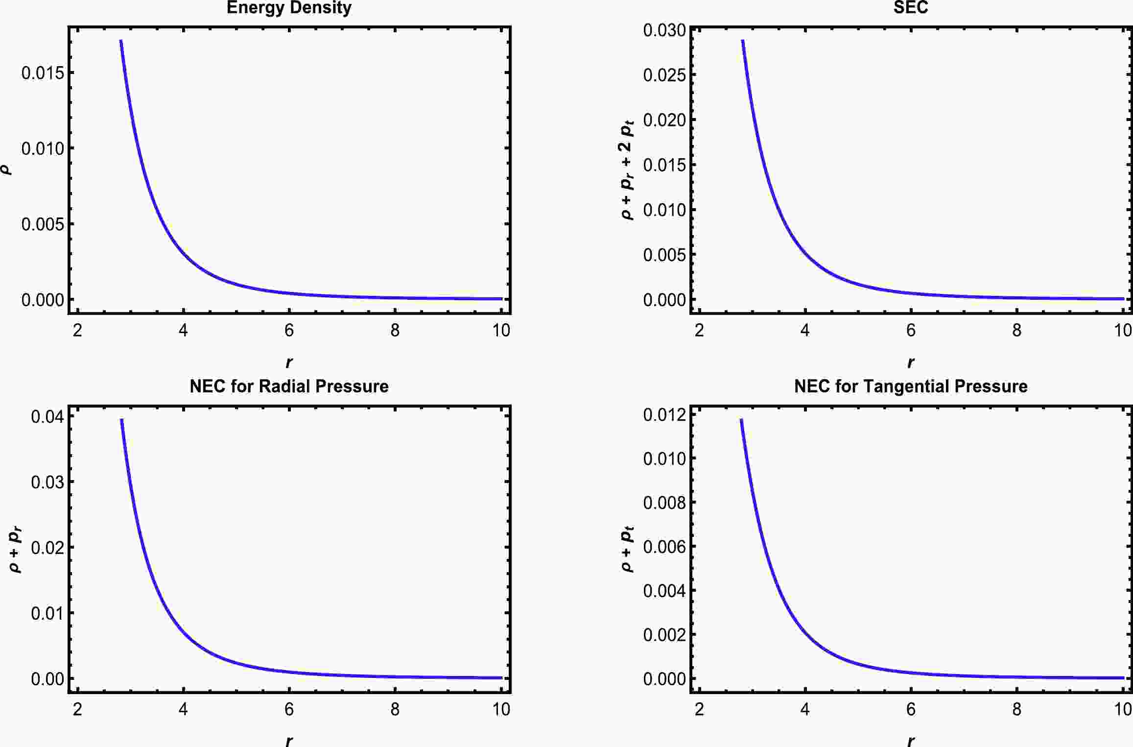
$ \phi_{4c}\,<\phi_0\,<{\rm{min}}\left[F_+\left(\dfrac{r_0}{r}\right)\right] $ .Now, considering the above analysis, we explore two examples of solutions. The first satisfies the NEC, WEC, and SEC, as shown in Fig. 1, and the second is for the solution satisfying all the ECs, i.e., the NEC, WEC, SEC, and DEC, as shown in Fig. 2. This is done by considering several particular values of α, β, λ, η, and
$ \phi_0 $ .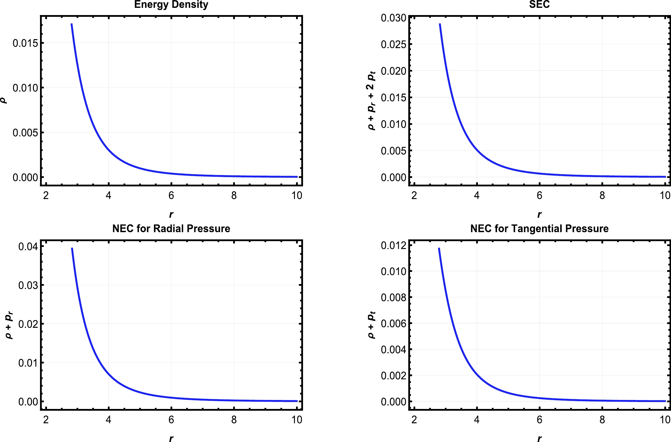
Figure 1. (color online) Profile shows the behavior of the NEC, WEC, and SEC for
$ \alpha = 1 $ ,$ \beta = -9 \pi $ ,$ \eta = 2 $ ,$ \lambda = 4 $ ,$ r_0 = 2 $ , and$ \phi_0 = -0.05 $ .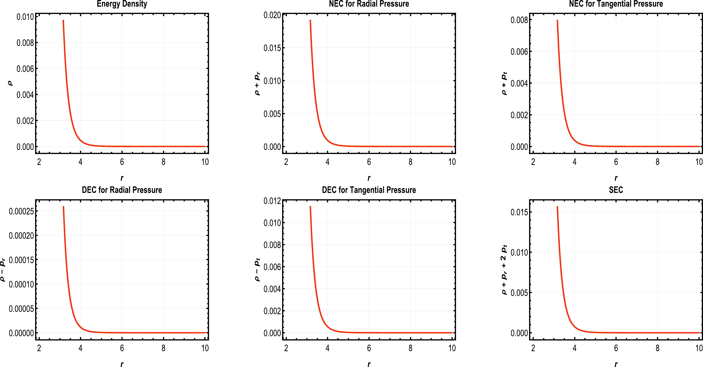
Figure 2. (color online) Profile shows the behavior of the NEC, WEC, SEC, and DEC for
$ \alpha = 1 $ ,$ \beta = -25.5 $ ,$ \eta = 10 $ ,$ \lambda = 12 $ ,$ r_0 = 2 $ , and$ \phi_0 = -0.0008 $ . -
In this section, we consider the following non-linear form of
$ f(Q,T) $ [77]:$ \begin{equation} f(Q,T) = Q+\gamma\,Q^2+\mu\,T \,, \end{equation} $

(82) where γ and μ are model parameters.
Moreover, we choose the same redshift function
$ \phi(r) $ and shape function$ b(r) $ as used in the linear model given by Eqs. (19) and (20). Using a non-linear form of$ f(Q,T) $ , a particular form of the redshift and shape function, energy density ρ, radial pressure$ p_r $ , and tangential pressure$ p_t $ are calculated from the field equations (Eqs. (15)−(17)) and written as$ \begin{aligned}[b] \rho = &\frac{1}{12 (4 \pi -\mu ) (\mu +8 \pi ) r^6 \left(r-r_0 \left(\frac{r_0}{r}\right)^{\eta }\right)^2}\left[r r_0^3 \left(\frac{r_0}{r}\right)^{3 \eta } \left(\lambda \phi _0 \left(\frac{r_0}{r}\right)^{\lambda } \left(\mu \left(2 \gamma \left(5 \eta ^2+20 (\eta +1) \lambda +34 \eta +49\right) \right.\right.\right.\right.\\& \left.\left.\left.\left. +r^2 (5 \eta +10 \lambda -11)\right)+10 \lambda \mu \phi _0 \left(\frac{r_0}{r}\right)^{\lambda } \left(4 \gamma (\eta +1)+r^2\right)-48 \pi \left(2 \gamma (\eta +1)+r^2\right)\right)-4 (12 \pi -\mu ) \left(2 \gamma (\eta +2)^2 \right.\right.\right. \\& \left.\left.\left. +\eta r^2\right)\right) +2 r^2 r_0^2 \left(\frac{r_0}{r}\right)^{2 \eta } \left(\lambda \phi _0 \left(\frac{r_0}{r}\right)^{\lambda } \left(-5 \lambda \mu \phi _0 \left(\frac{r_0}{r}\right)^{\lambda } \left(2 \gamma (\eta +1)+3 r^2\right)-\mu \left(10 \gamma (\eta (\lambda +2)+\lambda +3)+r^2 (5 \eta \right.\right.\right.\right. \\& \left.\left.\left.\left. +15 \lambda -16)\right)+48 \pi r^2\right) +4 \eta (12 \pi -\mu ) r^2\right)+r^6 \left(\frac{r_0}{r}\right)^{\eta +1} \left(4 \eta (\mu -12 \pi )+\lambda \phi _0 \left(\frac{r_0}{r}\right)^{\lambda } \left(\mu (5 \eta +30 \lambda -31)+30 \lambda \right.\right.\right. \\& \left.\left.\left. \mu \phi _0 \left(\frac{r_0}{r}\right)^{\lambda }-48 \pi \right)\right)-10 \lambda \mu r^6 \phi _0 \left(\frac{r_0}{r}\right)^{\lambda } \left(\lambda +\lambda \phi _0 \left(\frac{r_0}{r}\right)^{\lambda }-1\right)+\gamma r_0^4 \left(\frac{r_0}{r}\right)^{4 \eta } \left(-(\eta (11 \eta +30)+27) \mu +24 \pi \right.\right. \\& \left.\left. (\eta (3 \eta +10)+11)+2 \lambda \phi _0 \left(\frac{r_0}{r}\right)^{\lambda }\left(-\mu \left(5 \eta ^2+10 (\eta +1) \lambda +14 \eta +19\right)+48 \pi (\eta +1)-10 (\eta +1) \lambda \mu \phi _0 \left(\frac{r_0}{r}\right)^{\lambda }\right)\right)\right] \,, \end{aligned} $

(83) $ \begin{aligned}[b] p_r =& \frac{1}{12 (4 \pi -\mu ) (\mu +8 \pi ) r^6 \left(r-r_0 \left(\frac{r_0}{r}\right)^{\eta }\right)^2}\left[r r_0^3 \left(\frac{r_0}{r}\right)^{3 \eta } \left(\lambda \phi _0 \left(\frac{r_0}{r}\right)^{\lambda } \left(-\mu \left(2 \gamma \left(5 \eta ^2+20 (\eta +1) \lambda +82 \eta +97\right) \right.\right.\right.\right.\\& \left.\left.\left.\left. +r^2 (5 \eta +10 \lambda +13)\right)-10 \lambda \mu \phi _0 \left(\frac{r_0}{r}\right)^{\lambda } \left(4 \gamma (\eta +1)+r^2\right)+48 \pi \left(10 \gamma (\eta +1)+3 r^2\right)\right)+4 \mu \left(4 \gamma \eta (\eta +1)-2 \gamma + \right.\right.\right.\\& \left.\left.\left. (2 \eta +3) r^2\right)-48 \pi \left(r^2-2 \gamma (2 \eta +3)\right)\right)+2 r^2 r_0^2 \left(\frac{r_0}{r}\right)^{2 \eta } \left(\lambda \phi _0 \left(\frac{r_0}{r}\right)^{\lambda } \left(2 \gamma \mu (5 (\eta +1) \lambda +22 \eta +27)+5 \lambda \mu \phi _0 \left(\frac{r_0}{r}\right)^{\lambda } \right.\right.\right.\\& \left.\left.\left. \left(2 \gamma (\eta +1)+3 r^2\right)-96 \pi \left(\gamma \eta +\gamma +2 r^2\right)+5 \mu r^2 (\eta +3 \lambda +4)\right)+4 r^2 (12 \pi -(2 \eta +3) \mu )\right)+r^6 \left(\frac{r_0}{r}\right)^{\eta +1} \left(4 (2 \eta +3) \right.\right.\\& \left.\left. \mu -\lambda \phi _0 \left(\frac{r_0}{r}\right)^{\lambda } \left(\mu (5 \eta +30 \lambda +41)+30 \lambda \mu \phi _0 \left(\frac{r_0}{r}\right)^{\lambda }-336 \pi \right)-48 \pi \right)+2 \lambda r^6 \phi _0 \left(\frac{r_0}{r}\right)^{\lambda } \left(5 \lambda \mu +7 \mu +5 \lambda \mu \phi _0 \left(\frac{r_0}{r}\right)^{\lambda } \right.\right.\\& \left.\left. -48 \pi \right)+\gamma r_0^4 \left(\frac{r_0}{r}\right)^{4 \eta } \left((3-\eta (13 \eta +18)) \mu +24 \pi ((\eta -2) \eta -7)+2 \lambda \phi _0 \left(\frac{r_0}{r}\right)^{\lambda } \left(\mu \left(5 \eta ^2+10 (\eta +1) \lambda +38 \eta +43\right) \right.\right.\right.\\& \left.\left.\left. -144 \pi (\eta +1)+10 (\eta +1) \lambda \mu \phi _0 \left(\frac{r_0}{r}\right)^{\lambda }\right)\right)\right] \,, \end{aligned} $

(84) $ \begin{aligned}[b] p_t =& \frac{1}{12 (4 \pi -\mu ) (\mu +8 \pi ) r^6 \left(r-r_0 \left(\frac{r_0}{r}\right)^{\eta }\right)^2}\left[2 r^2 r_0^2 \left(\frac{r_0}{r}\right)^{2 \eta } \left(\lambda \phi _0 \left(\frac{r_0}{r}\right)^{\lambda } \left(\lambda (24 \pi -\mu ) \phi _0 \left(\frac{r_0}{r}\right)^{\lambda } \left(2 \gamma (\eta +1)+3 r^2\right) \right.\right.\right.\\& \left.\left.\left. -\mu \left(2 \gamma (\eta (\lambda +8)+\lambda +9)+r^2 (\eta +3 \lambda +22)\right)+24 \pi \left(2 \gamma (\eta (\lambda +3)+\lambda +4)+r^2 (\eta +3 \lambda -1)\right)\right)-2 r^2 ((\eta -3) \mu \right.\right.\\& \left.\left. +12 \pi (\eta +1))\right)+r r_0^3 \left(\frac{r_0}{r}\right)^{3 \eta } \left(\lambda \phi _0 \left(\frac{r_0}{r}\right)^{\lambda } \left(-2 \lambda (24 \pi -\mu ) \phi _0 \left(\frac{r_0}{r}\right)^{\lambda } \left(4 \gamma (\eta +1)+r^2\right)+\mu \left(2 \gamma (\eta (\eta +4 \lambda +38)+ \right.\right.\right.\right.\\& \left.\left.\left.\left. 4 \lambda +41)+r^2 (\eta +2 \lambda +17)\right)-24 \pi \left(2 \gamma (\eta (\eta +4 \lambda +10)+4 \lambda +13)+r^2 (\eta +2 \lambda -1)\right)\right)+2 \mu \left(2 \gamma (\eta (\eta +10)+13) \right.\right.\right.\\& \left.\left.\left. +(\eta -3) r^2\right)+24 \pi (\eta +1) \left(2 \gamma (\eta +1)+r^2\right)\right)+r^6 \left(\frac{r_0}{r}\right)^{\eta +1} \left(2 (\eta -3) \mu +24 \pi (\eta +1)+\lambda \phi _0 \left(\frac{r_0}{r}\right)^{\lambda } \left(\mu (\eta +6 \lambda +37) \right.\right.\right.\\& \left.\left.\left. -24 \pi (\eta +6 \lambda -1)-6 \lambda (24 \pi -\mu ) \phi _0 \left(\frac{r_0}{r}\right)^{\lambda }\right)\right)+2 \lambda r^6 \phi _0 \left(\frac{r_0}{r}\right)^{\lambda } \left(-(\lambda +5) \mu +24 \pi \lambda +\lambda (24 \pi -\mu ) \phi _0 \left(\frac{r_0}{r}\right)^{\lambda }\right)+\gamma \right.\\ &\left. r_0^4 \left(\frac{r_0}{r}\right)^{4 \eta } \left(-(\eta (\eta +18)+33) \mu -24 \pi (\eta +1)^2+2 \lambda \phi _0 \left(\frac{r_0}{r}\right)^{\lambda } \left(-\mu (\eta (\eta +2 \lambda +22)+2 \lambda +23)+24 \pi (\eta (\eta +2 \lambda +4) \right.\right.\right.\\& \left.\left.\left. +2 \lambda +5)+2 (\eta +1) \lambda (24 \pi -\mu )\phi _0 \left(\frac{r_0}{r}\right)^{\lambda }\right)\right)\right] \,. \end{aligned} $

(85) Finding the NEC in the radial and tangential directions is made possible by the following components:
$ \begin{equation} \rho+p_r = -\frac{\left(r_0 \left(\frac{r_0}{r}\right)^{\eta } \left(2 \gamma (\eta +1) r_0 \left(\frac{r_0}{r}\right)^{\eta }-r^3\right)+r^4\right) \left(r_0 \left(\frac{r_0}{r}\right)^{\eta } \left(\eta -2 \lambda \phi _0 \left(\frac{r_0}{r}\right)^{\lambda }+1\right)+2 \lambda r \phi _0 \left(\frac{r_0}{r}\right)^{\lambda }\right)}{(\mu +8 \pi ) r^6 \left(r-r_0 \left(\frac{r_0}{r}\right)^{\eta }\right)} \,, \end{equation} $

(86) $ \begin{aligned}[b] \rho+p_t =& \frac{1}{2 (\mu +8 \pi ) r^6 \left(r-r_0 \left(\frac{r_0}{r}\right)^{\eta }\right)^2} \left[2 r^2 r_0^2 \left(\frac{r_0}{r}\right)^{2 \eta } \left(\lambda \phi _0 \left(\frac{r_0}{r}\right){}^{\lambda } \left(2 \gamma (\eta (\lambda +3)+\lambda +4)+\lambda \phi _0 \left(\frac{r_0}{r}\right)^{\lambda } \left(2 \gamma (\eta +1)+ \right.\right.\right.\right. \\& \left.\left.\left.\left. 3 r^2\right)+r^2 (\eta +3 \lambda +1)\right)+(\eta -1) r^2\right)-r r_0^3 \left(\frac{r_0}{r}\right)^{3 \eta } \left(2 \gamma (\eta (\eta +6)+7)+\lambda \phi _0 \left(\frac{r_0}{r}\right)^{\lambda } \left(2 \gamma (\eta (\eta +4 \lambda +12)+4 \lambda \right.\right.\right. \\& \left.\left.\left. +15)+2 \lambda \phi _0 \left(\frac{r_0}{r}\right)^{\lambda } \left(4 \gamma (\eta +1)+r^2\right)+r^2 (\eta +2 \lambda +1)\right)+(\eta -1) r^2\right)-r^6 \left(\frac{r_0}{r}\right)^{\eta +1} \left(\eta +\lambda \phi _0 \left(\frac{r_0}{r}\right)^{\lambda } \left(\eta +6 \lambda \right.\right.\right. \\& \left.\left.\left. +6 \lambda \phi _0 \left(\frac{r_0}{r}\right)^{\lambda }+1\right)-1\right)+2 \lambda ^2 r^6 \phi _0 \left(\frac{r_0}{r}\right)^{\lambda } \left(\phi _0 \left(\frac{r_0}{r}\right)^{\lambda }+1\right)+2 \gamma r_0^4 \left(\frac{r_0}{r}\right)^{4 \eta } \left(\eta (\eta +4)+\lambda \phi _0 \left(\frac{r_0}{r}\right)^{\lambda } \left(\eta (\eta +2 \lambda \right.\right.\right. \\& \left.\left.\left. +6) +2 \lambda +2 (\eta +1) \lambda \phi _0 \left(\frac{r_0}{r}\right)^{\lambda }+7\right)+5\right)\right] \,. \end{aligned} $

(87) In this particular instance, we observe that the NEC along the radial and tangential directions becomes undefinable at the WH's throat, or
$ r = r_0 $ . This demonstrates that WH solutions are impossible to achieve using this shape function (20). As a result, we draw the conclusion that postulating a non-linear form (82) is inappropriate for WH solutions with the shape function (20). Yet, there are other shape function options that we might explore more in the future. -
Because there are two different metrics across the thin shell to match the condition along the boundary, we must use the Israel junction condition to obtain the solutions (in general, we use the junction condition because, along hypersurfaces, the metric must be continuous as well as differentiable; therefore, we check both the Christoffel symbol and Riemann curvature tensor to see what the boundary condition leads to, because in thin shell formulation, we can obtain such a thing via the calculations performed below).
We also note that the thin shell or three-manifold would be denoted by Σ. Outside of the thin shell, there are Schwarzschild solutions denoted by
$ M^+ $ , and inside, there is a WH$ M^- $ , and the total space-time would be$ M^+\cup\Sigma\cup M^- $ . We can focus the stress σ and pressure p, construct the effective potential from this, and find the condition for certain exotic matter given the NEC violation.This can be done as follows. We have the interior solutions
$ \begin{equation} {\rm d}s^2 = {\rm e}^{2\phi(r)}{\rm d}t^2-(f(r))^{-1}{\rm d}r^2-r^2\,{\rm d}\theta^2-r^2\,\sin^2\theta\,{\rm d}\Phi^2\,. \end{equation} $

(88) For the exterior solutions, we take the Schwarzschild solution of the form
$ \begin{equation} {\rm d}s^2 = -F(r){\rm d}t^2+(F(r))^{-1}{\rm d}r^2+r^2+{\rm d}\Omega^2\,. \end{equation} $

(89) We also note that in both cases, the space-like component is spherically symmetric, and on the boundary, we can obtain the FLRW metric
$ \begin{equation} {\rm d}s^2 = -{\rm d}\tau^2+a(\tau)^2 {\rm d}\Omega^2\,. \end{equation} $

(90) Now, if we take the formula for the first junction condition, we get
$ \begin{equation} K_{ab}^{\pm} = -n_{\gamma}^{\pm}\left(\frac{\partial^2x^{\gamma}_{\pm}}{\partial \zeta^a \partial \zeta^b}+\Gamma^{\gamma}_{\alpha\beta}\frac{\partial x^{\alpha}_{\pm}}{d\zeta^a}\frac{\partial x^{\beta}_{\pm}}{d\zeta^b}\right)\,, \end{equation} $

(91) and using the first Israel junction condition, we can obtain the proper boundary condition.
For interior geometry, we obtain the following components:
$ \begin{equation} K^{\tau-}_{\tau} = \frac{f'(a)+2\ddot{a}}{2\sqrt{f(a)+\dot{a}}};\,\,\,\,\,\,\,\,\,K^{\theta-}_{\theta} = \frac{\sqrt{f(a)+\dot{a}^2}}{a};\,\,\,\,\,\,\,\,\, K^{\phi-}_{\phi} = \sin^2{\theta} K^{\theta-}_{\theta}\,. \end{equation} $

(92) For exterior geometry, we obtain the following components:
$ \begin{equation} K^{\tau+}_{\tau} = \frac{F'(a)+2\ddot{a}}{2\sqrt{F(a)+\dot{a}}};\,\,\,\,\,\,\,\,\,K^{\theta+}_{\theta} = \frac{\sqrt{F(a)+\dot{a}^2}}{a};\,\,\,\,\,\,\,\,\,K^{\phi+}_{\phi} = \sin^2{\theta} K^{\theta+}_{\theta}\,, \end{equation} $

(93) where a dot denotes the derivative with respect to the proper time (τ), and a prime denotes the derivative with respect to ordinary time.
Now, to calculate the surface stress and pressure for the thin shell to sustain itself, we use the Lankoz equation
$ \begin{equation} S_{ab} = \frac{1}{8\pi}\left[g_{ab}K-K_{ab}\right]\,, \end{equation} $

(94) where
$ a,b = 0,2,3 $ because, at the shell, r is constant,$ \begin{equation} \sigma(a) = -\frac{1}{4\pi a}\left[\sqrt{F(a)+\dot{a}^2}-\sqrt{f(a)+\dot{a}^2}\right] \end{equation} $

(95) and
$ \begin{aligned}[b] p(a) =& \frac{1}{16\pi a}\Bigg[\frac{2F(a)+aF'(a)+2a\ddot{a}+2\dot{a}^2}{\sqrt{F(a)+\dot{a}^2}}\\&-\frac{2f(a)+af'(a)+2a\ddot{a}+2\dot{a}^2}{\sqrt{f(a)+\dot{a}^2}}\Bigg]\,. \end{aligned} $

(96) Note that at the throat
$ a = a_0 $ , we get$ \dot{a_0} = 0 $ ; hence, at the throat, we get$ \begin{equation} \sigma(a_0) = -\frac{1}{4\pi a_0}\left[\sqrt{F(a_0)}-\sqrt{f(a_0)}\right] \end{equation} $

(97) and also
$ \begin{equation} p(a_0) = \frac{1}{16\pi a_0}\left[\frac{2F(a_0)+a_0F'(a_0)}{\sqrt{F(a_0)}}-\frac{2f(a_0)+a_0f'(a_0)}{\sqrt{f(a_0)}}\right]\,. \end{equation} $

(98) Note that at the throat, the NEC must be violated. In other words,
$ \sigma(a_0)+p(a_0)<0 $ at the throat. The violation of the NEC on the shell would imply the presence of exotic matter.By following the prescription given by [72, 73], we can go further and calculate the potential
$ V(r) $ by noting that the energy-momentum has a conservation relation,$ \begin{equation} \frac{\rm d}{{\rm d}\tau}(\sigma \phi) = p\frac{{\rm d}\phi}{{\rm d}\tau} = 0\,, \end{equation} $

(99) where
$ \sigma = 4\pi a^2 $ . From the conservation equation above, we can find$ \begin{equation} \sigma ' = -\frac{2}{a}(\sigma+p)\,. \end{equation} $

(100) Following the prescription given in [66], the last equation has the form
$ \dot{a}^2+V(a) $ ; therefore, from the above equation, we can get$ \begin{equation} V(a) = \frac{f(a)}{2}+\frac{F(a)}{2}-\frac{(f(a)-F(a))^2}{64a^2\pi^2\sigma^2}-4a^2\pi^2\sigma^2\,. \end{equation} $

(101) We also note that in our case,
$ f(r) $ and$ F(r) $ are given by the following:$ f(r) = 1-\frac{b(r)}{r} $

and
$ F(r) = 1-\frac{2GM}{r} $

Outside the thin shell, we can take the Schwarzschild solution because there is no matter, and hence, the Schwarzschild solution is applicable in a vacuum with spherical symmetry.
Figure 3 shows that a thin shell in the junction feels a similar potential (in natural units) to that of a massive particle in the Schwarzschild metric.
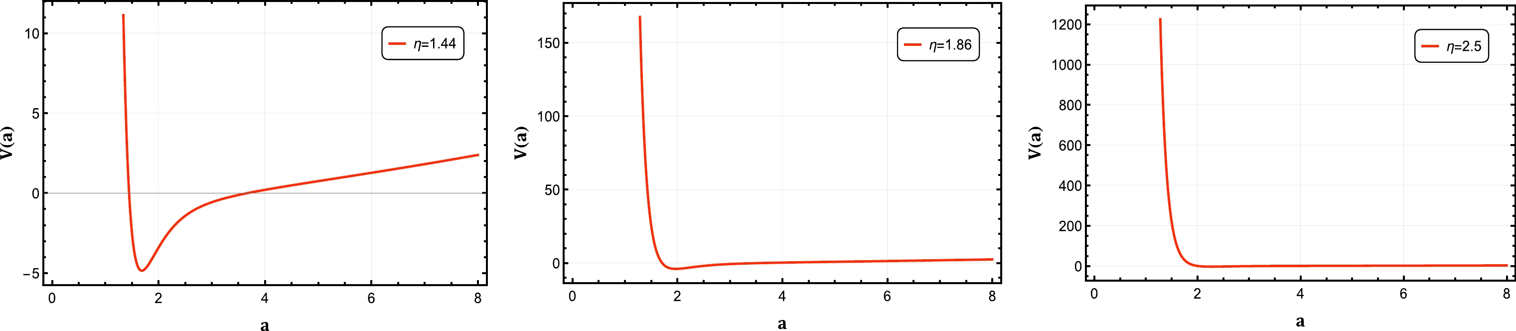
Figure 3. (color online) Profile shows the behaviour of
$ V(a) $ for$ M =0.2 $ and$ a_0 =3.68 $ . -
The present study involves a comprehensive analytical investigation of the parameter space for a particular family of WH solutions within the framework of the linear
$ f(Q, T) = \alpha Q + \beta T $ theory of gravity. The main objective is to determine the necessary constraints on the free parameters of the model that ensure the traversability and non-exoticity of the WH solutions, which implies that all ECs are satisfied across the entire spacetime. Additionally, we demonstrate that even in cases where some parameter bounds are exceeded, resulting in the WH becoming exotic beyond the throat at a finite radius$ r_c $ , such exoticity can be effectively eliminated through a spacetime matching an exterior vacuum solution.We consider a family of WHs with a redshift and shape function described by the expressions in Eqs. (19) and (20), respectively, within a linear version of
$ f(Q, T) = \alpha Q + \beta T $ theory. Our main finding is that ensuring the WH solution satisfies the NEC for the entire spacetime automatically guarantees that the WEC and SEC are also satisfied. This is because the parameter bounds arising from the ECs$ \rho > 0 $ and$ \rho + p_r + 2p_t > 0 $ are weaker than those arising from$ \rho + p_i > 0 $ . However, it should be noted that the implications are one-directional, and thus a solution satisfying$ \rho > 0 $ or$ \rho + p_r + 2p_t > 0 $ may not necessarily satisfy the NEC for the entire spacetime. Regarding the DEC, we show that the bounds arising from$ \rho-p_i > 0 $ are stronger than those from$ \rho + p_i > 0 $ , which means that a solution satisfying the NEC may not necessarily satisfy the DEC. Nonetheless, we demonstrate that strong solutions satisfying all four ECs (NEC, WEC, SEC, and DEC) can be achieved for a wide range of parameter combinations. Our choice of the linear form$ f(Q, T) $ enables us to perform an analytical study of the parameter space and prove that even the simplest extension of GR within the framework of$ f(R, T) $ can effectively address the issue of exotic matter in WH spacetimes.In the paper, we also show the stability of the thin-shell around a WH. We calculate the stress (σ) and pressure (P) of such a thin shell. Furthermore, we find the conditions under which the thin-shell has exotic matter (by checking the NEC). We also show that, by using the energy-momentum conservation equation, we can find the potential (
$ V(a) $ ) across the thin shell. We draw the shape of V for various values of η and reveal that it exhibits a similar behavior to what a particle feels outside the Schwarzchild radius. This potential can be used to calculate the gravitational lensing, accretion disk (via ISCO), etc., of such a thin shell. From the observation of gravitational lensing and phenomena around a thin shell composed of dust, one can reconstruct the potential and obtain the shape function using backward bootstrap. -
There are no new data associated with this article.
-
We are very grateful to the honorable referee and editor for their illuminating suggestions that have significantly improved our work in terms of research quality and presentation.
Non-exotic static spherically symmetric thin-shell wormhole solution in f (Q, T ) gravity
- Received Date: 2023-03-23
- Available Online: 2023-07-15
Abstract: In this study, we conduct an analysis of traversable wormhole solutions within the framework of linear


 DownLoad: