


 Abstract
 HTML
HTML Reference
 Related
 PDF
PDF


-
Recently, many single heavy baryons have been observed in experiments, and the mass spectra of single heavy baryon families have become increasingly abundant [1−29]. Such a wealth of experimental data gives theorists an opportunity to test the validity of current theoretical frameworks. In addition, this is a good time to carry out systematic and precise calculations using theoretical methods, for promoting the consistency between experiments and theories.
The strange single heavy baryon
$ \Xi_{Q} $ families including$ \Xi_{c} $ ($ \Xi_{c}^{'} $ ) [1−14] and$ \Xi_{b} $ ($ \Xi_{b}^{'} $ ) [16−25], are being established step by step, owing to the cooperative efforts of experimentalists and theorists. So far, more than a dozen$ \Xi_{Q} $ baryons have been recorded in the latest particle data group (PDG) [28], even though the$ J^{P} $ values of some baryons remain undetermined, such as those of$ \Xi_{c}(3055) $ ,$ \Xi_{c}(3080) $ and$ \Xi_{c}(6227) $ . Recently, some other$ \Xi_{Q} $ baryons have been observed in experiments, including$ \Xi_{c}(3123) $ [4],$ \Xi_{c}(2930) $ [12],$ \Xi_{c}(2923) $ ,$ \Xi_{c}(2939) $ ,$ \Xi_{c}(2964) $ [13],$ \Xi_{b}(6327) $ and$ \Xi_{b}(6333) $ [25]. Accordingly, many theoretical studies have been performed on these baryons, such as$ \Xi_{c}(3055) $ [30−34],$ \Xi_{c}(3080) $ [34, 35],$ \Xi_{c}(2923)^{0} $ (including$ \Xi_{c}(2939)^{0} $ and$ \Xi_{c}(2965)^{0} $ ) [36],$ \Xi_{c}(2930)^{0} $ [37],$ \Xi_{c}(2970) $ [38−41],$ \Xi_{c} $ (3123) [42],$ \Xi_{b}(6227) $ [43−47],$ \Xi_{b}(6100) $ [48, 49], and$ \Xi_{b}(6327) $ ($ \Xi_{b}(6333) $ ) [50]. For identifying their quantum numbers and for assigning them suitable positions in the mass spectra, it is necessary to systematically investigate their spectroscopies.In recent decades, heavy baryons have been studied using many theoretical methods, including the quark potential model in the heavy quark-light diquark picture [42,51−54], relativistic quark model [55], harmonic oscillator quark model [36], constituent quark model [56−63], chiral quark model [30, 37, 43, 50], chiral perturbation theory [64−68], relativistic flux tube model[42], Bethe-Salpeter formalism [69], effective Lagrangian approach [44],
$ ^{3}P_{0} $ decay model [70−77], lattice quantum chromodynamics (QCD) [78−81], bound state picture [82], light cone QCD sum rules [83−92], and QCD sum rules [93−102].In particular, it is worth mentioning that Ebert
$ et\ al. $ [51, 52] put forward a heavy quark-light diquark picture in the framework of a QCD-motivated relativistic quark model, in which an initial three-body problem was reduced to a two-step two-body problem. They systematically studied the spectroscopy and Regge trajectories of heavy baryons and successfully predicted new single heavy baryons. Because the excited states in the heavy quark-light diquark picture are very similar to those of the λ-mode in a three-quark system [60], it would be interesting to investigate the λ-mode in the three-quark system systematically and study the differences between the mass spectra of this mode and the heavy quark-light diquark picture.In the 1980s, Godfrey and Isgur developed a relativistic quark model, using which they studied the mass spectra of mesons [103]. Then, Capstick and Isgur extended the model to baryons [55]. In the relativistic quark model, the Hamiltonian contains almost all of the interactions between two quarks, which is expected to give accurate calculations for heavy baryon spectra.
The Gaussian expansion method (GEM) and the infinitesimally-shifted Gaussian (ISG) basis functions [104] have been successfully applied to few-body systems in nuclear physics. The ISG method is advantageous for improving the computational accuracy and efficiency associated with the calculations of few-body systems. Recently, they were introduced in the study of heavy baryons [60−62], tetraquarks [105−107] and pentaquarks [108].
Inspired by the above discussion, we combined the relativistic quark model with the ISG method, for investigating the strange single heavy baryon spectra of a three-quark system. For the excited states, we only focused on the λ-mode and compared the results with those of the heavy quark-light diquark picture and some relevant experimental data. The present work is a preliminary attempt to systematically investigate strange single heavy baryon spectra; the method is promising for studying other multi-quark systems, including the exotic ones [109−113].
The remainder of this paper is organized as follows. In Sec. II, we briefly describe the methods used in our theoretical calculations, mainly including the relativistic quark model and the GEM(ISG) method. In Sec. III, we present the root mean square radii and the mass spectra of the
$ \Xi_{Q} $ baryons, analyze the radial probability distributions, and construct the Regge trajectories. Based on these, we analyze in detail the baryons of recent interest. Finally, the mass spectral structures are demonstrated. Sec. IV lists our conclusions. -
The relativistic quark model is based on the hypothesis that baryons may be approximately described in terms of center-of-mass (CM) frame valence-quark configurations, the dynamics of which are governed by a Hamiltonian with a one-gluon exchange dominant component at short distances and with a confinement implemented by a flavor-independent Lorentz-scalar interaction [55]. For a three-quark system, the Hamiltonian reads
$ \begin{array}{*{20}{l}} \begin{aligned} &H=H_{0}+V, \end{aligned} \end{array} $

(1) $ \begin{array}{*{20}{l}} \begin{aligned} &H_{0}=\sum_{i=1}^{3}(p_{i}^{2}+m_{i}^{2})^{1/2},\\ \end{aligned} \end{array} $

(2) $ \begin{array}{*{20}{l}} \begin{aligned} &V=\sum _{i<j}(\tilde{H}^{\rm conf}_{ij}+\tilde{H}^{\rm so}_{ij}+\tilde{H}^{\rm hyp}_{ij}), \end{aligned} \end{array} $

(3) where
$ \tilde{H}^{\rm conf}_{ij} $ ,$ \tilde{H}^{\rm so}_{ij} $ , and$ \tilde{H}^{\rm hyp}_{ij} $ are the confinement, spin-orbit, and hyperfine interactions, respectively. The confinement item includes one-gluon exchange potentials and the linear confined potentials. Due to the relativistic effect, the interactions should be modified with CM momentum-dependent factors. It is worth noting that the forms of the interactions in this paper have been rearranged for ease of use [105, 114]. The interactions were decomposed as follows:$ \begin{eqnarray} &\tilde{H}^{\rm conf}_{ij}=G'_{ij}(r)+\tilde{S}_{ij}(r), \end{eqnarray} $

(4) $ \begin{eqnarray} &\tilde{H}^{\rm so}_{ij}=\tilde{H}^{{\rm so}(v)}_{ij}+\tilde{H}^{{\rm so}(s)}_{ij}, \end{eqnarray} $

(5) $ \begin{eqnarray} &\tilde{H}^{\rm hyp}_{ij}=\tilde{H}^{\rm tensor}_{ij}+\tilde{H}^{c}_{ij}, \end{eqnarray} $

(6) with
$ \tilde{H}^{{\rm so}(v)}_{ij} = \frac{ {S}_{i}\cdot {L}_{ij}}{2m^{2}_{i}r_{ij}}\frac{\partial\tilde{G}^{{\rm so}(v)}_{ii}}{\partial{r_{ij}}} + \frac{ {S}_{j}\cdot {L}_{ij}}{2m^{2}_{j}r_{ij}}\frac{\partial\tilde{G}^{{\rm so}(v)}_{jj}}{\partial{r_{ij}}} + \frac{( {S}_{i}+ {S}_{j})\cdot {L}_{ij}}{m_{i}m_{j}r_{ij}}\frac{\partial\tilde{G}^{{\rm so}(v)}_{ij}}{\partial{r_{ij}}}, $

(7) $ \begin{eqnarray} &\tilde{H}^{{\rm so}(s)}_{ij}=-\frac{ {S}_{i}\cdot {L}_{ij}}{2m^{2}_{i}r_{ij}}\frac{\partial\tilde{S}^{{\rm so}(s)}_{ii}}{\partial{r_{ij}}}- \frac{ {S}_{j}\cdot {L}_{ij}}{2m^{2}_{j}r_{ij}}\frac{\partial\tilde{S}^{{\rm so}(s)}_{jj}}{\partial{r_{ij}}}, \end{eqnarray} $

(8) $ \begin{eqnarray} &\tilde{H}^{\rm tensor}_{ij}=-\frac{ {S}_{i}\cdot {r}_{ij} {S}_{j}\cdot {r}_{ij}/r^{2}_{ij}-\dfrac{1}{3} {S}_{i}\cdot {S}_{j}}{m_{i}m_{j}} \times\left(\frac{\partial^{2}}{\partial{r^{2}_{ij}}}-\frac{1}{r_{ij}}\frac{\partial}{\partial{r_{ij}}}\right)\tilde{G}^{t}_{ij}, \end{eqnarray} $

(9) $ \tilde{H}^{c}_{ij}=\frac{2 {S}_{i}\cdot {S}_{j}}{3m_{i}m_{j}}\nabla^{2}\tilde{G}^{c}_{ij}. $

(10) The modified terms in Eqs. (4), (7), (8), (9), and (10) are
$ G'_{ij}=\left(1+\frac{p^{2}_{ij}}{E_{i}E_{j}}\right)^{\frac{1}{2}}\tilde{G}_{ij}(r_{ij})\left(1+\frac{p^{2}_{ij}}{E_{i}E_{j}}\right)^{\frac{1}{2}}, $

(11) $ \tilde{G}^{{\rm so}(v)}_{ij}=\left(\frac{m_{i}m_{j}}{E_{i}E_{j}}\right)^{\frac{1}{2}+\epsilon_{{\rm so}(v)}}\tilde{G}_{ij}(r_{ij})\left(\frac{m_{i}m_{j}}{E_{i}E_{j}}\right)^{\frac{1}{2}+\epsilon_{{\rm so}(v)}}, $

(12) $ \tilde{S}^{{\rm so}(s)}_{ii}=\left(\frac{m_{i}m_{i}}{E_{i}E_{i}}\right)^{\frac{1}{2}+\epsilon_{{\rm so}(s)}}\tilde{S}_{ij}(r_{ij})\left(\frac{m_{i}m_{i}}{E_{i}E_{i}}\right)^{\frac{1}{2}+\epsilon_{{\rm so}(s)}}, $

(13) $ \tilde{G}^{t}_{ij}=\left(\frac{m_{i}m_{j}}{E_{i}E_{j}}\right)^{\frac{1}{2}+\epsilon_{t}}\tilde{G}_{ij}(r_{ij})\left(\frac{m_{i}m_{j}}{E_{i}E_{j}}\right)^{\frac{1}{2}+\epsilon_{t}}, $

(14) $ \tilde{G}^{c}_{ij}=\left(\frac{m_{i}m_{j}}{E_{i}E_{j}}\right)^{\frac{1}{2}+\epsilon_{c}}\tilde{G}_{ij}(r_{ij})\left(\frac{m_{i}m_{j}}{E_{i}E_{j}}\right)^{\frac{1}{2}+\epsilon_{c}}, $

(15) where
$ E_{i}=\sqrt{m^{2}_{i}+p^{2}_{ij}} $ is the relativistic kinetic energy, and$ p_{ij} $ is the momentum magnitude of either of the quarks in the CM frame of the$ ij $ quark subsystem [105].$ \tilde{G}_{ij}(r_{ij}) $ and$ \tilde{S}_{ij}(r_{ij}) $ are obtained using the smearing transformations of the one-gluon exchange potential$ G(r)=-\dfrac{4\alpha_{s}(r)}{3r} $ and linear confinement potential$ S(r)= br+c $ , respectively,$ \tilde{G}_{ij}(r_{ij})= {F}_{i}\cdot {F}_{j}\sum^{3}_{k=1}\frac{2\alpha_{k}}{\sqrt{\pi}r_{ij}}\int^{\tau_{kij}r_{ij}}_{0}{\rm e} ^{-x^{2}}\mathrm{d}x, $

(16) $ \begin{aligned}[b] \tilde{S}_{ij}(r_{ij})=&-\frac{3}{4} {F}_{i}\cdot {F}_{j}\Bigg\{br_{ij}\Bigg[\frac{{\rm e}^{-\sigma^{2}_{ij}r^{2}_{ij}}}{\sqrt{\pi}\sigma_{ij} r_{ij}}\\&+\left(1+\frac{1}{2\sigma^{2}_{ij}r^{2}_{ij}}\right)\frac{2}{\sqrt{\pi}}\int^{\sigma_{ij}r_{ij}}_{0}{\rm e}^{-x^{2}}\mathrm{d}x\Bigg]+c\Bigg\}, \end{aligned} $

(17) with
$ \tau_{kij}=\frac{1}{\sqrt{\dfrac{1}{\sigma^{2}_{ij}}+\dfrac{1}{\gamma^{2}_{k}}}}, $

(18) $ \sigma_{ij}=\sqrt{s^{2}\left(\frac{2m_{i}m_{j}}{m_{i}+m_{j}}\right)^{2}+\sigma^{2}_{0}\left(\frac{1}{2}\left(\frac{4m_{i}m_{j}}{(m_{i}+m_{j})^{2}}\right)^{4}+\frac{1}{2}\right)}. $

(19) Here,
$ \alpha_{k} $ and$ \gamma_{k} $ are constants.$ {F}_{i}\cdot {F}_{j} $ stands for the inner product of the color matrices of quarks i and j.$ {F} $ includes 8 components (the so-called Gell-mann matrices), which can be written as$ \begin{split} F_{n}=\left \{ \begin{array}{ll} \dfrac{\hat{\lambda}_{n}}{2}, & \mathrm{for\ quarks},\\ -\dfrac{\hat{\lambda}^{*}_{n}}{2}, &\mathrm{ for\ antiquarks}, \end{array} \right. \end{split} $

(20) with
$ n=1,\cdot\cdot\cdot,8 $ . All of the parameters in these formulas were taken from Table 2 of Ref. [103], except that b and c were revised to 0.14 GeV$ ^{2} $ and –0.198 GeV, respectively. Using the revised b and c values, and setting the values of the other parameters as in Ref. [103], we can reproduce most of the experimental values nicely for single heavy baryons, such as$ \Lambda_{c,b} $ ,$ \Sigma_{c,b} $ ,$ \Omega_{c,b} $ (see Ref. [115]) and$ \Xi_{c,b} $ (see Tables 1−2 and 4−5 in the appendix of this article).$ l_{\rho} l_{\lambda} L s j $ 

$ nL $ (

$ J^{P} $ )

$ \langle r_{\rho}^{2}\rangle^{1/2} $ 

$ \langle r_{\lambda}^{2}\rangle^{1/2} $ 

mass exp.[28] [52] [56] [57] [58] 0 0 0 0 0 $ 1S $ (

$ \frac{1}{2}^{+} $ )

0.512 0.437 2479 $\Xi_{c}^{+}$ 2467.71(0.23)

$\Xi_{c}^{0}$ 2470.44(0.28)

2476 2466 2470 2471 $ 2S $ (

$ \frac{1}{2}^{+} $ )

0.645 0.768 2949 $ \Xi_{c}(2970) $ ?

2959 2940 2964 $ 3S $ (

$ \frac{1}{2}^{+} $ )

0.968 0.607 3155 3123?[4] 3323 3265 3358 $ 4S $ (

$ \frac{1}{2}^{+} $ )

0.690 1.131 3318 3632 3720 0 1 1 0 1 $ 1P $ (

$ \frac{1}{2}^{-} $ )

0.542 0.627 2789 2791.9(0.5)
2793.9(0.5)2792 2773 2793 2796 $ 2P $ (

$ \frac{1}{2}^{-} $ )

0.615 0.948 3176 3179 3140 3191 $ 3P $ (

$ \frac{1}{2}^{-} $ )

1.038 0.763 3390 3500 3541 $ 4P $ (

$ \frac{1}{2}^{-} $ )

0.655 1.285 3492 3785 3879 0 1 1 0 1 $ 1P $ (

$ \frac{3}{2}^{-} $ )

0.550 0.654 2819 2816.51(0.25)
2819.79(0.30)2819 2783 2820 2820 $ 2P $ (

$ \frac{3}{2}^{-} $ )

0.613 0.977 3199 3201 3164 3184 $ 3P $ (

$ \frac{3}{2}^{-} $ )

1.053 0.779 3412 3519 3533 $ 4P $ (

$ \frac{3}{2}^{-} $ )

0.645 1.278 3508 3804 3871 0 2 2 0 2 $ 1D $ (

$ \frac{3}{2}^{+} $ )

0.561 0.825 3063 3059 3012 3033 3116 $ 2D $ (

$ \frac{3}{2}^{+} $ )

0.601 1.161 3406 3388 3464 $ 3D $ (

$ \frac{3}{2}^{+} $ )

1.084 0.936 3617 3678 3804 $ 4D $ (

$ \frac{3}{2}^{+} $ )

0.627 1.349 3676 3945 4132 0 2 2 0 2 $ 1D $ (

$ \frac{5}{2}^{+} $ )

0.565 0.843 3076 3076 3004 3040 3103 $ 2D $ (

$ \frac{5}{2}^{+} $ )

0.604 1.190 3419 3407 3452 $ 3D $ (

$ \frac{5}{2}^{+} $ )

1.092 0.945 3627 3699 3792 $ 4D $ (

$ \frac{5}{2}^{+} $ )

0.618 1.328 3688 3965 4121 0 3 3 0 3 $ 1F $ (

$ \frac{5}{2}^{-} $ )

0.567 0.998 3289 3278 3388 $ 2F $ (

$ \frac{5}{2}^{-} $ )

0.604 1.413 3613 3572 3727 $ 3F $ (

$ \frac{5}{2}^{-} $ )

1.103 1.087 3817 3845 4055 $ 4F $ (

$ \frac{5}{2}^{-} $ )

0.602 1.314 3861 4098 4376 0 3 3 0 3 $ 1F $ (

$ \frac{7}{2}^{-} $ )

0.569 1.009 3294 3292 3369 $ 2F $ (

$ \frac{7}{2}^{-} $ )

0.607 1.439 3619 3592 3710 $ 3F $ (

$ \frac{7}{2}^{-} $ )

1.111 1.088 3821 3865 4042 $ 4F $ (

$ \frac{7}{2}^{-} $ )

0.589 1.290 3871 4120 4364 0 4 4 0 4 $ 1G $ (

$ \frac{7}{2}^{+} $ )

0.566 1.147 3486 3469 3215 3647 $ 2G $ (

$ \frac{7}{2}^{+} $ )

0.612 1.676 3798 3745 3981 $ 3G $ (

$ \frac{7}{2}^{+} $ )

1.121 1.205 4000 4303 $ 4G $ (

$ \frac{7}{2}^{+} $ )

0.559 1.222 4054 0 4 4 0 4 $ 1G $ (

$ \frac{9}{2}^{+} $ )

0.567 1.154 3487 3483 3627 $ 2G $ (

$ \frac{9}{2}^{+} $ )

0.613 1.692 3799 3763 3960 $ 3G $ (

$ \frac{9}{2}^{+} $ )

1.126 1.208 4001 4285 $ 4G $ (

$ \frac{9}{2}^{+} $ )

0.551 1.202 4064 Table 1. Root mean square radii (fm) and the mass spectra (MeV) of the
$ \Xi_{c} $ family.$l_{\rho} l_{\lambda} L s j$ 

$nL$ (

$J^{P}$ )

$\langle r_{\rho}^{2}\rangle^{1/2}$ 

$\langle r_{\lambda}^{2}\rangle^{1/2}$ 

mass [52] [56] [57] [58] 0 2 2 1 2 $1D$ (

$\frac{3}{2}^{+}$ )

0.668 0.851 3201 3160 3089 3121 $2D$ (

$\frac{3}{2}^{+}$ )

0.744 1.195 3541 3497 3469 $3D$ (

$\frac{3}{2}^{+}$ )

1.104 0.955 3676 3308 $4D$ (

$\frac{3}{2}^{+}$ )

0.738 1.303 3816 4136 0 2 2 1 2 $1D$ (

$\frac{5}{2}^{+}$ )

0.671 0.865 3211 3166 3080 3077 $2D$ (

$\frac{5}{2}^{+}$ )

0.745 1.219 3551 3504 $3D$ (

$\frac{5}{2}^{+}$ )

1.111 0.963 3685 $4D$ (

$\frac{5}{2}^{+}$ )

0.734 1.285 3828 0 2 2 1 3 $1D$ (

$\frac{5}{2}^{+}$ )

0.667 0.850 3200 3153 3091 3108 $2D$ (

$\frac{5}{2}^{+}$ )

0.744 1.193 3540 3493 3457 $3D$ (

$\frac{5}{2}^{+}$ )

1.104 0.954 3676 3796 $4D$ (

$\frac{5}{2}^{+}$ )

0.738 1.304 3815 4125 0 2 2 1 3 $1D$ (

$\frac{7}{2}^{+}$ )

0.672 0.868 3213 3147 3094 3078 3092 $2D$ (

$\frac{7}{2}^{+}$ )

0.746 1.224 3552 3486 3442 $3D$ (

$\frac{7}{2}^{+}$ )

1.112 0.965 3686 3782 $4D$ (

$\frac{7}{2}^{+}$ )

0.733 1.281 3829 4112 0 3 3 1 2 $1F$ (

$\frac{3}{2}^{-}$ )

0.676 1.022 3424 3418 3408 $2F$ (

$\frac{3}{2}^{-}$ )

0.742 1.454 3744 3745 $3F$ (

$\frac{3}{2}^{-}$ )

1.136 1.096 3872 4069 $4F$ (

$\frac{3}{2}^{-}$ )

0.699 1.262 4010 4388 0 3 3 1 2 $1F$ (

$\frac{5}{2}^{-}$ )

0.678 1.031 3428 3408 $2F$ (

$\frac{5}{2}^{-}$ )

0.744 1.474 3748 $3F$ (

$\frac{5}{2}^{-}$ )

1.140 1.101 3876 $4F$ (

$\frac{5}{2}^{-}$ )

0.698 1.243 4020 0 3 3 1 3 $1F$ (

$\frac{5}{2}^{-}$ )

0.676 1.022 3424 3394 2989 3393 $2F$ (

$\frac{5}{2}^{-}$ )

0.742 1.454 3744 3732 $3F$ (

$\frac{5}{2}^{-}$ )

1.136 1.096 3872 4059 $4F$ (

$\frac{5}{2}^{-}$ )

0.699 1.263 4009 4379 0 3 3 1 3 $1F$ (

$\frac{7}{2}^{-}$ )

0.678 1.031 3428 3393 $2F$ (

$\frac{7}{2}^{-}$ )

0.744 1.475 3748 $3F$ (

$\frac{7}{2}^{-}$ )

1.140 1.101 3876 $4F$ (

$\frac{7}{2}^{-}$ )

0.698 1.242 4021 0 3 3 1 4 $1F$ (

$\frac{7}{2}^{-}$ )

0.676 1.021 3423 3373 3375 $2F$ (

$\frac{7}{2}^{-}$ )

0.742 1.453 3744 3715 $3F$ (

$\frac{7}{2}^{-}$ )

1.136 1.095 3872 4046 $4F$ (

$\frac{7}{2}^{-}$ )

0.699 1.264 4009 4368 0 3 3 1 4 $1F$ (

$\frac{9}{2}^{-}$ )

0.678 1.032 3428 3357 3358 $2F$ (

$\frac{9}{2}^{-}$ )

0.744 1.476 3749 3695 $3F$ (

$\frac{9}{2}^{-}$ )

1.140 1.102 3876 4030 $4F$ (

$\frac{9}{2}^{-}$ )

0.698 1.241 4021 4354 Table 3. Root mean square radii (fm) and the mass spectra (MeV) of the
$\Xi^{'}_{c}$ family (Part II).$ l_{\rho} l_{\lambda} L s j $ 

$ nL $ (

$ J^{P} $ )

$ \langle r_{\rho}^{2}\rangle^{1/2} $ 

$ \langle r_{\lambda}^{2}\rangle^{1/2} $ 

mass [52] [56] [59] 0 2 2 1 2 $ 1D $ (

$ \frac{3}{2}^{+} $ )

0.656 0.773 6460 6431 6245 $ 2D $ (

$ \frac{3}{2}^{+} $ )

0.690 0.992 6758 6751 6439 $ 3D $ (

$ \frac{3}{2}^{+} $ )

1.109 0.845 6941 6610 $ 4D $ (

$ \frac{3}{2}^{+} $ )

0.754 1.464 7017 6763 0 2 2 1 2 $ 1D $ (

$ \frac{5}{2}^{+} $ )

0.658 0.780 6466 6432 6393 $ 2D $ (

$ \frac{5}{2}^{+} $ )

0.690 0.999 6764 6751 $ 3D $ (

$ \frac{5}{2}^{+} $ )

1.112 0.851 6946 $ 4D $ (

$ \frac{5}{2}^{+} $ )

0.751 1.462 7021 0 2 2 1 3 $ 1D $ (

$ \frac{5}{2}^{+} $ )

0.656 0.773 6460 6420 6241 $ 2D $ (

$ \frac{5}{2}^{+} $ )

0.690 0.991 6757 6740 6437 $ 3D $ (

$ \frac{5}{2}^{+} $ )

1.108 0.844 6941 6609 $ 4D $ (

$ \frac{5}{2}^{+} $ )

0.754 1.464 7017 6762 0 2 2 1 3 $ 1D $ (

$ \frac{7}{2}^{+} $ )

0.658 0.781 6467 6414 6395 6237 $ 2D $ (

$ \frac{7}{2}^{+} $ )

0.690 1.000 6765 6736 6434 $ 3D $ (

$ \frac{7}{2}^{+} $ )

1.112 0.851 6946 6607 $ 4D $ (

$ \frac{7}{2}^{+} $ )

0.751 1.461 7021 6761 0 3 3 1 2 $ 1F $ (

$ \frac{3}{2}^{-} $ )

0.663 0.931 6657 6675 6341 $ 2F $ (

$ \frac{3}{2}^{-} $ )

0.678 1.121 6942 6527 $ 3F $ (

$ \frac{3}{2}^{-} $ )

1.130 0.986 7110 $ 4F $ (

$ \frac{3}{2}^{-} $ )

0.734 1.580 7162 0 3 3 1 2 $ 1F $ (

$ \frac{5}{2}^{-} $ )

0.664 0.936 6660 6686 $ 2F $ (

$ \frac{5}{2}^{-} $ )

0.680 1.130 6946 $ 3F $ (

$ \frac{5}{2}^{-} $ )

1.131 0.991 7114 $ 4F $ (

$ \frac{5}{2}^{-} $ )

0.732 1.573 7164 0 3 3 1 3 $ 1F $ (

$ \frac{5}{2}^{-} $ )

0.663 0.931 6657 6640 6337 $ 2F $ (

$ \frac{5}{2}^{-} $ )

0.678 1.121 6942 6524 $ 3F $ (

$ \frac{5}{2}^{-} $ )

1.130 0.986 7110 $ 4F $ (

$ \frac{5}{2}^{-} $ )

0.734 1.580 7162 0 3 3 1 3 $ 1F $ (

$ \frac{7}{2}^{-} $ )

0.664 0.936 6660 6641 $ 2F $ (

$ \frac{7}{2}^{-} $ )

0.680 1.131 6947 $ 3F $ (

$ \frac{7}{2}^{-} $ )

1.131 0.991 7114 $ 4F $ (

$ \frac{7}{2}^{-} $ )

0.731 1.572 7165 0 3 3 1 4 $ 1F $ (

$ \frac{7}{2}^{-} $ )

0.663 0.931 6657 6619 6333 $ 2F $ (

$ \frac{7}{2}^{-} $ )

0.678 1.121 6942 6524 $ 3F $ (

$ \frac{7}{2}^{-} $ )

1.130 0.986 7110 $ 4F $ (

$ \frac{7}{2}^{-} $ )

0.734 1.580 7162 0 3 3 1 4 $ 1F $ (

$ \frac{9}{2}^{-} $ )

0.664 0.937 6661 6610 6328 $ 2F $ (

$ \frac{9}{2}^{-} $ )

0.680 1.132 6947 6519 $ 3F $ (

$ \frac{9}{2}^{-} $ )

1.131 0.991 7114 $ 4F $ (

$ \frac{9}{2}^{-} $ )

0.731 1.572 7165 Table 6. Root mean square radii (fm) and the mass spectra (MeV) of the
$ \Xi^{'}_{b} $ family (Part II).$l_{\rho} l_{\lambda} L s j$ 

$nL$ (

$J^{P}$ )

$\langle r_{\rho}^{2}\rangle^{1/2}$ 

$\langle r_{\lambda}^{2}\rangle^{1/2}$ 

mass exp.[28] [52] [56] [57] [58] 0 0 0 1 1 $1S$ (

$\frac{1}{2}^{+}$ )

0.590 0.431 2590 $\Xi_{c}^{'+}$ 2578.2(0.5)

$\Xi_{c}^{'0}$ 2578.7(0.5)

2579 2594 2579 $2S$ (

$\frac{1}{2}^{+}$ )

0.821 0.705 3046 $\Xi_{c}(3055)$ ?

2983 2977 $3S$ (

$\frac{1}{2}^{+}$ )

0.918 0.671 3201 3377 3215 $4S$ (

$\frac{1}{2}^{+}$ )

0.897 1.053 3425 3695 0 0 0 1 1 $1S$ (

$\frac{3}{2}^{+}$ )

0.611 0.476 2658 2645.10(0.30)
2646.16(0.25)2654 2649 2649 2648 $2S$ (

$\frac{3}{2}^{+}$ )

0.801 0.763 3095 $\Xi_{c}(3080)$ ?

3026 3007 3080 $3S$ (

$\frac{3}{2}^{+}$ )

0.968 0.676 3244 3396 3236 3424 $4S$ (

$\frac{3}{2}^{+}$ )

0.850 1.095 3456 3709 3763 0 1 1 1 0 $1P$ (

$\frac{1}{2}^{-}$ )

0.649 0.671 2952 2936 2900 $2P$ (

$\frac{1}{2}^{-}$ )

0.762 0.978 3326 3313 3144 $3P$ (

$\frac{1}{2}^{-}$ )

1.055 0.811 3469 3630 $4P$ (

$\frac{1}{2}^{-}$ )

0.783 1.245 3636 3912 0 1 1 1 1 $1P$ (

$\frac{1}{2}^{-}$ )

0.644 0.659 2941 2854 2855 2839 2832 $2P$ (

$\frac{1}{2}^{-}$ )

0.763 0.962 3315 3267 3094 3195 $3P$ (

$\frac{1}{2}^{-}$ )

1.048 0.804 3460 3598 3545 $4P$ (

$\frac{1}{2}^{-}$ )

0.788 1.248 3628 3887 3883 0 1 1 1 1 $1P$ (

$\frac{3}{2}^{-}$ )

0.651 0.677 2958 2935 2866 2932 $2P$ (

$\frac{3}{2}^{-}$ )

0.761 0.985 3331 3311 3165 $3P$ (

$\frac{3}{2}^{-}$ )

1.059 0.814 3473 3628 $4P$ (

$\frac{3}{2}^{-}$ )

0.780 1.243 3640 3911 0 1 1 1 2 $1P$ (

$\frac{3}{2}^{-}$ )

0.642 0.653 2934 2912 2921 2824 $2P$ (

$\frac{3}{2}^{-}$ )

0.764 0.955 3310 3293 3172 3188 $3P$ (

$\frac{3}{2}^{-}$ )

1.043 0.801 3456 3613 3537 $4P$ (

$\frac{3}{2}^{-}$ )

0.791 1.249 3624 3898 3875 0 1 1 1 2 $1P$ (

$\frac{5}{2}^{-}$ )

0.652 0.682 2964 2929 2895 2927 2814 $2P$ (

$\frac{5}{2}^{-}$ )

0.761 0.993 3335 3303 3170 3177 $3P$ (

$\frac{5}{2}^{-}$ )

1.062 0.817 3477 3619 3527 $4P$ (

$\frac{5}{2}^{-}$ )

0.778 1.241 3644 3902 3865 0 2 2 1 1 $1D$ (

$\frac{1}{2}^{+}$ )

0.668 0.851 3201 3163 3075 3131 $2D$ (

$\frac{1}{2}^{+}$ )

0.744 1.195 3541 3505 3478 $3D$ (

$\frac{1}{2}^{+}$ )

1.104 0.955 3676 3817 $4D$ (

$\frac{1}{2}^{+}$ )

0.738 1.303 3816 4144 0 2 2 1 1 $1D$ (

$\frac{3}{2}^{+}$ )

0.671 0.865 3211 3167 3081 $2D$ (

$\frac{3}{2}^{+}$ )

0.745 1.219 3550 3506 $3D$ (

$\frac{3}{2}^{+}$ )

1.111 0.963 3684 $4D$ (

$\frac{3}{2}^{+}$ )

0.734 1.285 3827 Table 2. Root mean square radii (fm) and the mass spectra (MeV) of the
$\Xi^{'}_{c}$ family (Part I).$ l_{\rho} l_{\lambda} L s j $ 

$ nL $ (

$ J^{P} $ )

$ \langle r_{\rho}^{2}\rangle^{1/2} $ 

$ \langle r_{\lambda}^{2}\rangle^{1/2} $ 

mass exp.[28] [52] [56] [59] 0 0 0 0 0 $ 1S $ (

$ \frac{1}{2}^{+} $ )

0.518 0.400 5806 $\Xi_{c}^{+}$ 2467.71(0.23)

$\Xi_{c}^{0}$ 2470.44(0.28)

5803 5806 5796 $ 2S $ (

$ \frac{1}{2}^{+} $ )

0.607 0.705 6224 6266 6208 $ 3S $ (

$ \frac{1}{2}^{+} $ )

0.990 0.549 6480 6601 6533 $ 4S $ (

$ \frac{1}{2}^{+} $ )

0.672 1.066 6568 6913 6825 0 1 1 0 1 $ 1P $ (

$ \frac{1}{2}^{-} $ )

0.539 0.571 6084 6120 6090 6137 $ 2P $ (

$ \frac{1}{2}^{-} $ )

0.586 0.844 6421 6496 6341 $ 3P $ (

$ \frac{1}{2}^{-} $ )

1.034 0.713 6690 6805 6520 $ 4P $ (

$ \frac{1}{2}^{-} $ )

0.673 1.281 6732 7068 6679 0 1 1 0 1 $ 1P $ (

$ \frac{3}{2}^{-} $ )

0.543 0.583 6097 6100.3(0.6) 6130 6093 6135 $ 2P $ (

$ \frac{3}{2}^{-} $ )

0.585 0.853 6432 6502 6339 $ 3P $ (

$ \frac{3}{2}^{-} $ )

1.043 0.719 6700 6810 6519 $ 4P $ (

$ \frac{3}{2}^{-} $ )

0.668 1.293 6739 7073 6678 0 2 2 0 2 $ 1D $ (

$ \frac{3}{2}^{+} $ )

0.551 0.743 6320 6366 6311 6243 $ 2D $ (

$ \frac{3}{2}^{+} $ )

0.568 0.962 6613 6690 6438 $ 3D $ (

$ \frac{3}{2}^{+} $ )

0.990 1.040 6883 6966 6610 $ 4D $ (

$ \frac{3}{2}^{+} $ )

0.778 1.359 6890 7208 6762 0 2 2 0 2 $ 1D $ (

$ \frac{5}{2}^{+} $ )

0.553 0.751 6327 6373 6300 6240 $ 2D $ (

$ \frac{5}{2}^{+} $ )

0.568 0.967 6621 6696 6436 $ 3D $ (

$ \frac{5}{2}^{+} $ )

0.948 1.124 6888 6970 6608 $ 4D $ (

$ \frac{5}{2}^{+} $ )

0.831 1.294 6894 7212 6761 0 3 3 0 3 $ 1F $ (

$ \frac{5}{2}^{-} $ )

0.555 0.903 6518 6577 6313 6336 $ 2F $ (

$ \frac{5}{2}^{-} $ )

0.553 1.064 6795 6863 6524 $ 3F $ (

$ \frac{5}{2}^{-} $ )

0.619 1.646 7032 7114 $ 4F $ (

$ \frac{5}{2}^{-} $ )

1.110 0.960 7057 7339 0 3 3 0 3 $ 1F $ (

$ \frac{7}{2}^{-} $ )

0.556 0.909 6523 6581 6331 $ 2F $ (

$ \frac{7}{2}^{-} $ )

0.553 1.070 6801 6867 6521 $ 3F $ (

$ \frac{7}{2}^{-} $ )

0.618 1.641 7034 7117 $ 4F $ (

$ \frac{7}{2}^{-} $ )

1.111 0.965 7060 7342 0 4 4 0 4 $ 1G $ (

$ \frac{7}{2}^{+} $ )

0.554 1.048 6692 6760 6517 $ 2G $ (

$ \frac{7}{2}^{+} $ )

0.542 1.178 6970 7020 $ 3G $ (

$ \frac{7}{2}^{+} $ )

0.607 1.745 7167 $ 4G $ (

$ \frac{7}{2}^{+} $ )

1.119 1.095 7214 0 4 4 0 4 $ 1G $ (

$ \frac{9}{2}^{+} $ )

0.555 1.052 6695 6762 $ 2G $ (

$ \frac{9}{2}^{+} $ )

0.544 1.189 6975 7032 $ 3G $ (

$ \frac{9}{2}^{+} $ )

0.605 1.737 7169 $ 4G $ (

$ \frac{9}{2}^{+} $ )

1.120 1.098 7217 Table 4. Root mean square radii (fm) and the mass spectra (MeV) of the
$ \Xi_{b} $ family.$l_{\rho} l_{\lambda} L s j$ 

$nL$ (

$J^{P}$ )

$\langle r_{\rho}^{2}\rangle^{1/2}$ 

$\langle r_{\lambda}^{2}\rangle^{1/2}$ 

mass exp.[28] [52] [56] [59] 0 0 0 1 1 $1S$ (

$\frac{1}{2}^{+}$ )

0.604 0.411 5943 5935.02(0.05) 5936 5970 5935 $2S$ (

$\frac{1}{2}^{+}$ )

0.741 0.697 6350 6329 6328 $3S$ (

$\frac{1}{2}^{+}$ )

0.998 0.559 6535 6687 6625 $4S$ (

$\frac{1}{2}^{+}$ )

0.804 1.063 6691 6978 6902 0 0 0 1 1 $1S$ (

$\frac{3}{2}^{+}$ )

0.614 0.431 5971 5952.3(0.6)
5955.33(0.13)5963 5980 5958 $2S$ (

$\frac{3}{2}^{+}$ )

0.735 0.716 6370 6342 6343 $3S$ (

$\frac{3}{2}^{+}$ )

1.017 0.566 6554 6695 6634 $4S$ (

$\frac{3}{2}^{+}$ )

0.793 1.087 6705 6984 6907 0 1 1 1 0 $1P$ (

$\frac{1}{2}^{-}$ )

0.642 0.608 6238 6233 6188 $2P$ (

$\frac{1}{2}^{-}$ )

0.709 0.866 6569 6611 $3P$ (

$\frac{1}{2}^{-}$ )

1.074 0.705 6758 6915 $4P$ (

$\frac{1}{2}^{-}$ )

0.772 1.296 6866 7174 0 1 1 1 1 $1P$ (

$\frac{1}{2}^{-}$ )

0.640 0.603 6232 6227 6138 $2P$ (

$\frac{1}{2}^{-}$ )

0.709 0.862 6564 6604 $3P$ (

$\frac{1}{2}^{-}$ )

1.071 0.701 6754 6904 6521 $4P$ (

$\frac{1}{2}^{-}$ )

0.774 1.292 6863 7164 6679 0 1 1 1 1 $1P$ (

$\frac{3}{2}^{-}$ )

0.643 0.610 6240 6234 $2P$ (

$\frac{3}{2}^{-}$ )

0.709 0.868 6572 6605 $3P$ (

$\frac{3}{2}^{-}$ )

1.076 0.707 6760 6905 $4P$ (

$\frac{3}{2}^{-}$ )

0.771 1.297 6868 7163 0 1 1 1 2 $1P$ (

$\frac{3}{2}^{-}$ )

0.639 0.600 6229 6227.9(0.9)?
6226.8(1.6)?6224 6190 6136 $2P$ (

$\frac{3}{2}^{-}$ )

0.709 0.859 6562 6598 6340 $3P$ (

$\frac{3}{2}^{-}$ )

1.069 0.700 6752 6900 6520 $4P$ (

$\frac{3}{2}^{-}$ )

0.774 1.291 6861 7159 6678 0 1 1 1 2 $1P$ (

$\frac{5}{2}^{-}$ )

0.644 0.613 6243 6226 6201 6133 $2P$ (

$\frac{5}{2}^{-}$ )

0.708 0.871 6574 6596 6338 $3P$ (

$\frac{5}{2}^{-}$ )

1.077 0.708 6762 6897 6518 $4P$ (

$\frac{5}{2}^{-}$ )

0.770 1.299 6869 7156 6677 0 2 2 1 1 $1D$ (

$\frac{1}{2}^{+}$ )

0.656 0.773 6460 6447 6247 $2D$ (

$\frac{1}{2}^{+}$ )

0.690 0.992 6757 6767 6440 $3D$ (

$\frac{1}{2}^{+}$ )

1.109 0.845 6941 6611 $4D$ (

$\frac{1}{2}^{+}$ )

0.754 1.464 7017 6763 0 2 2 1 1 $1D$ (

$\frac{3}{2}^{+}$ )

0.658 0.780 6466 6459 $2D$ (

$\frac{3}{2}^{+}$ )

0.690 0.998 6763 6775 $3D$ (

$\frac{3}{2}^{+}$ )

1.111 0.850 6946 $4D$ (

$\frac{3}{2}^{+}$ )

0.751 1.462 7020 Table 5. Root mean square radii (fm) and the mass spectra (MeV) of the
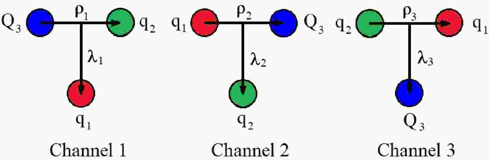
$ \Xi^{'}_{b} $ family (Part I).To represent the internal motion of quarks in a few-body system, one commonly introduces the Jacobi coordinates. As shown in Fig. 1, there are overall three channels of the Jacobi coordinates for the three-body system. The corresponding Jacobi coordinates are defined as

Figure 1. (color online) Jacobi coordinates for the three-quark system. We denote the heavy quark as the third one in the case of single heavy baryons.
$ \boldsymbol\rho_{i}= {r}_{j}- {r}_{k}, $

(21) $ \boldsymbol\lambda_{i}= {r}_{i}-\frac{m_{j} {r}_{j}+m_{k} {r}_{k}}{m_{j}+m_{k}}, $

(22) where i, j, k = 1, 2, 3 (or replace their positions in turn).
$ {r}_{i} $ and$ m_{i} $ denote the position vector and the mass of the ith quark, respectively.We perform our calculations based on channel 3. In this case, the third quark is just the heavy quark, which is consistent with the heavy quark limit [116, 117]. Further,
$ {l}_{\rho3} $ (denoted succinctly as$ {l}_{\rho} $ ) is clearly defined as the orbital angular momentum between the light quarks, and$ {l}_{\lambda3} $ (denoted succinctly as$ {l}_{\lambda} $ ) represents the one between the heavy quark and the light-quark pair. -
In the heavy quark limit, the heavy quark within the heavy baryon system is decoupled from the two light quarks. With the requirement of the flavor SU(3) subgroups for the light quarks, the baryons belong to either a sextet
$ (6_{F}) $ of flavor-symmetric states$ \Xi_{Q}^{'} $ or an antitriplet$ (\bar{3}_{F}) $ of flavor antisymmetric states$ \Xi_{Q} $ . The flavor wave functions of strange single heavy baryons are$ \begin{aligned}[b] & \Xi_{Q}^{'}=\frac{1}{\sqrt{2}}(qq_{s}+q_{s}q)Q, \\ & \Xi_{Q}=\frac{1}{\sqrt{2}}(qq_{s}-q_{s}q)Q. \end{aligned} $

(23) Here q denotes an up or down quark, and Q is a charm or bottom quark, while
$ q_{s} $ is a strange quark. For a quantum state with specified angular momenta in this work, the spatial wave function is combined with the spin function, as follows:$ \begin{aligned}[b]& |l_{\rho} \ l_{\lambda} \ L \ s\ j\ J\ M_{J}\rangle \\=&\sum^{1/2}_{m_{s3}=-1/2}\sum^{j}_{m_{j}=-j}\sum^{L}_{M_{L}=-L}\sum^{s}_{m_{s}=-s}\sum^{1/2}_{m_{s1}=-1/2}\sum^{1/2}_{m_{s2}=-1/2} \sum^{l_{\rho}}_{m_{\rho}=-l_{\rho}}\sum^{l_{\lambda}}_{m_{\lambda}=-l_{\lambda}}\\ &\ \times\langle j\ m_{j}\ s_{3}\ m_{s_{3}}| j\ s_{3}\ J\ M_{J}\rangle\times \langle L\ M_{L}\ s\ m_{s}| L\ s\ j\ m_{j}\rangle\\ &\times\langle s_{1}\ m_{s_{1}}\ s_{2}\ m_{s_{2}}| s_{1}\ s_{2}\ s\ m_{s}\rangle\times \langle l_{\rho}\ m_{\rho} l_{\lambda}\ m_{\lambda}| l_{\rho}\ l_{\lambda}\ L\ M_{L}\rangle\\ &\times |l_{\rho}\ m_{\rho} \rangle\otimes |l_{\lambda}\ m_{\lambda} \rangle\otimes |s_{1}\ m_{s_{1}} \rangle\otimes |s_{2}\ m_{s_{2}} \rangle \otimes |s_{3}\ m_{s_{3}} \rangle , \end{aligned} $

(24) with
$ {L}= {l}_{\rho}+ {l}_{\lambda} $ ,$ {s}= {s}_{1}+ {s}_{2} $ ,$ {j}= {L}+ {s} $ , and$ {J}= {j}+ {s}_{3} $ .$ l_{\rho} $ ,$ l_{\lambda} $ , L, s, j, J, and$ M_{J} $ are the quantum numbers that characterize a given quantum state in theory. This scheme$ |l_{\rho} \ l_{\lambda} \ L \ s\ j\ J\ M_{J}\rangle $ (j-s coupling) is also commonly used for analyzing the strong decay of heavy baryons [74]. -
In calculations, the spatial wave function
$ |l_{\rho}\ m_{\rho} \rangle\otimes |l_{\lambda}\ m_{\lambda} \rangle $ in formula (24) should be expanded in terms of basis functions. Naturally, one of the candidates is the simple harmonic oscillator (SHO) basis, owing to its good orthogonality. However, the completeness of the SHO is not rigorous in calculations because a truncated set has to be used [55, 103]. Compared with the SHO basis functions, the advantage of the Gaussian basis functions is that they can form an approximately complete set in a finite coordinate space. This is known as the GEM [104].Following formula (24), the spatial wave function is expanded in terms of a set of Gaussian basis functions,
$ \begin{eqnarray} \begin{aligned} |l_{\rho} m_{\rho} \rangle\otimes |l_{\lambda} m_{\lambda} \rangle=\sum_{n_{\rho}=1}^{n_{\max}}\sum_{n_{\lambda}=1}^{n_{\max}}c_{n_{\rho}n_{\lambda}}|n_{\rho} l_{\rho} m_{\rho} \rangle^{G} \otimes |n_{\lambda} l_{\lambda} m_{\lambda} \rangle^{G}, \end{aligned} \end{eqnarray} $

(25) where the Gaussian basis function
$ |nlm \rangle^{G} $ is commonly written in the position space as$ \begin{aligned}[b] &\phi^{G}_{nlm}( {r})=\phi^{G}_{nl}(r)Y_{lm}(\hat{ {r}}),\\ &\phi^{G}_{nl}(r)=N_{nl}r^{l}{\rm e}^{-\nu_{n}r^{2}},\\ &N_{nl}=\sqrt{\frac{2^{l+2}(2\nu_{n})^{l+3/2}}{\sqrt{\pi}(2l+1)!!}}, \end{aligned} $

(26) or in the momentum space as
$ \begin{aligned}[b] &\phi^{\prime G}_{nlm}( {p})=\phi^{\prime G}_{nl}(p)Y_{lm}(\hat{ {p}}),\\ &\phi^{\prime G}_{nl}(p)=N'_{nl}p^{l}{\rm e}^{-\frac{p^{2}}{4\nu_{n}}},\\ &N'_{nl}=(-i)^{l}\sqrt{\frac{2^{l+2}}{\sqrt{\pi}(2\nu_{n})^{l+3/2}(2l+1)!!}}, \end{aligned} $

(27) with
$ \begin{aligned}[b] & \nu_{n}=\frac{1}{r^{2}_{n}},\\ & r_{n}=r_{1}a^{n-1}\ \ \ (n=1,\ 2,\ ...,\ n_{\max}). \end{aligned} $

(28) $ r_{1} $ , a, and$n_{\max}$ are the Gaussian size parameters in the geometric progression for numerical calculations, and the final results are stable and independent of these parameters within an approximately complete set in a sufficiently large space.The Gaussian basis functions are non-orthogonal, which leads to a generalized matrix eigenvalue problem,
$ \begin{array}{*{20}{l}} \begin{aligned} \sum_{\kappa'=1}^{\kappa_{\max}}[H_{\kappa\kappa'}-E\tilde{N}_{\kappa\kappa'}]c_{\kappa'}=0, \end{aligned} \end{array} $

(29) with
$ \begin{aligned}[b] \tilde{N}_{\kappa\kappa'}=&\langle\phi^{G}_{n_{\rho}l_{\rho}m_{\rho}}|\phi^{G}_{n_{\rho'}l_{\rho'}m_{\rho'}}\rangle \times\langle\phi^{G}_{n_{\lambda}l_{\lambda}m_{\lambda}}|\phi^{G}_{n_{\lambda'}l_{\lambda'}m_{\lambda'}}\rangle \\ =&\left(\frac{2\sqrt{\nu_{n_{\rho}}\nu_{n_{\rho'}}}}{\nu_{n_{\rho}}+\nu_{n_{\rho'}}}\right)^{l_{\rho}+3/2} \times\left(\frac{2\sqrt{\nu_{n_{\lambda}}\nu_{n_{\lambda'}}}}{\nu_{n_{\lambda}}+\nu_{n_{\lambda'}}}\right)^{l_{\lambda}+3/2}, \end{aligned} $

(30) where
$\kappa=1,\ 2,...,\ \kappa_{\max}$ ,$\kappa_{\max}=n_{\max}\times n_{\max}$ and$ c_{\kappa}=c_{n_{\rho}n_{\lambda}} $ . H and E denote the Hamiltonian and the eigenvalue, respectively.In the calculation of the Hamiltonian matrix elements of three-body systems, particularly, when complicated interactions are employed, integrations over all of the radial and angular coordinates become laborious even with the Gaussian basis functions. This process can be simplified by introducing the ISG basis functions by
$ \phi_{nlm}^{G}( {r})=N_{nl}r^{l}{\rm e}^{-\nu_{n}r^{2}}Y_{lm}(\hat{ {r}}) =N_{nl}\lim_{\varepsilon\rightarrow0}\sum_{k=1}^{k_{\max}}C_{lm,k}{\rm e}^{-\nu_{n}( {r}-\varepsilon {D}_{lm,k})^{2}}. $

(31) In formula (31),
$ Y_{lm}(\hat{ {r}}) $ is replaced by a set of coefficients$ C_{lm,k} $ and vectors$ {D}_{lm,k} $ . Thus, the ISG method can effectively avoid the difficulty of spatial angle integration in the calculation of matrix elements. This method is described in detail in literature [104]. -
The Gaussian size parameters
$\{n_{\max},\ r_{1},\ r_{n_{\max}}\}$ are related to the scale in question. For example, they are different in Ref. [104] and Ref. [118]. To obtain stable numerical solutions in our calculation, they should be optimized specifically. For the Gaussian functions that constitute a set of non-orthogonal bases in a finite coordinate space, the number of the bases should be in a reasonable range. As shown in Fig. 2, the numerical stability is achieved when the dimension parameter$ n_{\max} $ is in the$ 9\sim14 $ range, with$ r_{1}=0.18 $ GeV$ ^{-1} $ and$r_{n_{\max}}= 15$ GeV$ ^{-1} $ . The value$n_{\max}=10$ was adopted in this work, using which both the computation efficiency and accuracy were actually satisfied.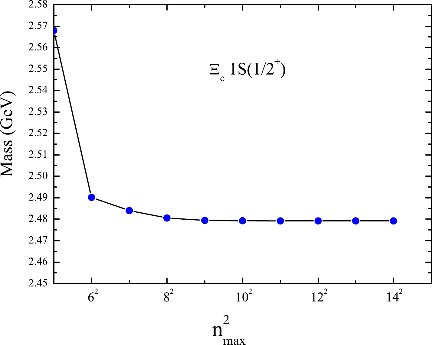
Figure 2. (color online) Numerical stability of the
$ \Xi_{c}1S(\dfrac{1}{2}^{+}) $ mass with respect to the dimension parameter$n_{\max}$ .$ nL(J^{P}) $ is commonly used to describe baryon states. For angular momentum$ L\neq0 $ , there exist several$ |l_{\rho} l_{\lambda} L s j J M_{J}\rangle $ states satisfying the condition$ {L}= {l}_{\rho}+ {l}_{\lambda} $ . They may be divided into the following three modes: (1) the ρ-mode with$ l_{\rho}\neq0 $ and$ l_{\lambda}=0 $ ; (2) the λ-mode with$ l_{\rho}=0 $ and$ l_{\lambda}\neq0 $ ; and (3) the λ-ρ mixing mode with$ l_{\rho}\neq0 $ and$ l_{\lambda}\neq0 $ .As an example, the excitation energies of the
$ 1P(\dfrac{1}{2}^{-}, \dfrac{3}{2}^{-})_{j=1} $ states of$ \bar{3}_{F} $ as functions of$ m_{Q} $ were investigated, where the dependence of excitation energies on$ m_{Q} $ of the λ-mode was compared with that of the ρ-mode. As shown in Fig. 3, the λ-mode and the ρ-mode became clearly separated when$ m_{Q} $ increased from 1.0 GeV to 5.0 GeV. In the case of$ 6_{F} $ , we reached the same conclusion for$ m_{Q}>1.5 $ GeV, as shown in Fig. 4. Besides the p-wave states, the same was observed for higher angular excited states [60]. Thus, we investigated the mass spectrum in the λ-mode.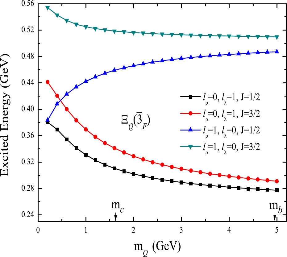
Figure 3. (color online) Dependence of the excitation energy on
$ m_{Q} $ , for different modes of$ \Xi_{Q} $ . The black and red curves represent the λ-mode. The blue and green ones denote the ρ-mode.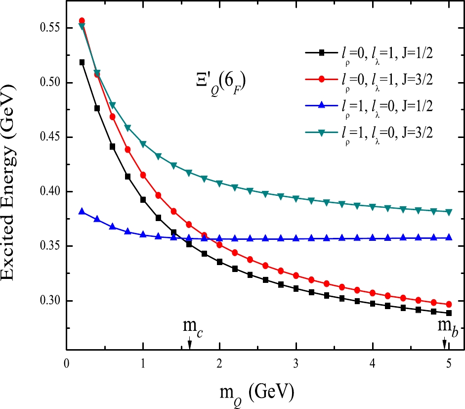
Figure 4. (color online) Excitation energy versus
$ m_{Q} $ , for different modes of$ \Xi_{Q}^{'} $ . Note that the black curve is lower than the blue one with$ m_{Q}>1.5 $ GeV, and the red curve is overall lower than the green one ($ m_{c}=1.628 $ GeV and$ m_{b}=4.977 $ GeV were used in this work). -
In this subsection, the root mean square radii, radial probability density distributions, and the mass spectra of strange single heavy baryons are presented. For convenience, the relevant experimental data are given together. The detailed results are listed in Tables 1−6 (see the appendix). There are overall four families, namely
$ \Xi_{c} $ ,$ \Xi_{c}^{'} $ ,$ \Xi_{b} $ and$ \Xi_{b}^{'} $ . The mass spectra of excited states with quantum numbers up to$ n=4 $ and$ L=4 $ are displayed. Many theoretical studies have been conducted on this subject [35, 44, 52, 56−59, 119, 120]. For reference, the results of some of these studies are included in the following tables.By analyzing these calculated results, some general features of the mass spectra were inferred, as follows. First,
$ \Xi_{Q} $ is lower than$ \Xi_{Q}^{'} $ in terms of the energy. This feature has been recognized in light baryons where highly orbitally excited states have an antisymmetric structure that minimizes the energy [121]. Second, the mass splitting of spin-doublet states decreases with increasing L. For example, Table 1 shows that the mass differences for the spin-doublets of$ 1P $ -,$ 1D $ -,$ 1F $ -, and$ 1G $ -wave are 30 MeV, 13 MeV, 5 MeV, and 1 MeV, respectively. Third, for the same L, the mass splitting hardly changes as j increases. For example, Tables 2 and 3 show that the mass differences for$ 1D $ doublets with$ j=1,2,3 $ are 10 MeV, 10 MeV, and 13 MeV, respectively. Finally, the mass difference between two adjacent radial excited states gradually decreases with increasing n, which is clearly different from that given by Ebert$ et\ al. $ .In addition, the calculated root mean square radii and radial probability density distributions carry important information. For a three-quark system, the radial probability densities
$ \omega(r_{\rho}) $ and$ \omega(r_{\lambda}) $ can be defined as follows:$ \begin{aligned}[b] & \omega(r_{\rho})=\int |\Psi( {r}_{\rho}, {r}_{\lambda})|^{2}\mathrm{d} {r}_{\lambda}\mathrm{d}\Omega_{\rho},\\ & \omega(r_{\lambda})=\int |\Psi( {r}_{\rho}, {r}_{\lambda})|^{2}\mathrm{d} {r}_{\rho}\mathrm{d}\Omega_{\lambda}, \end{aligned} $

(32) where
$ \Omega_{\rho} $ and$ \Omega_{\lambda} $ are the solid angles spanned by vectors$ {r}_{\rho} $ and$ {r}_{\lambda} $ , respectively. From Figs. 5−7 and Tables 1-6, one can observe some interesting properties.
Figure 5. (color online) Radial probability density distributions for some
$ 1L $ states in the$ \Xi_{c} $ and$ \Xi_{c}^{'} $ families. The solid line denotes the probability density with$ r_{\rho} $ , and the dashed line denotes the one with$ r_{\lambda} $ .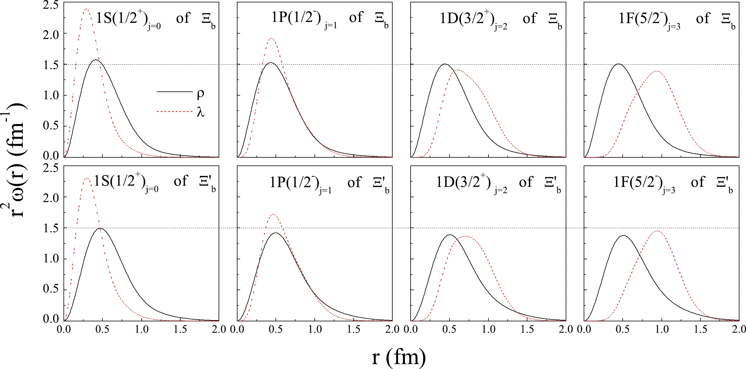
Figure 6. (color online) Same as for Fig. 5, but for the
$ \Xi_{b} $ and$ \Xi_{b}^{'} $ families.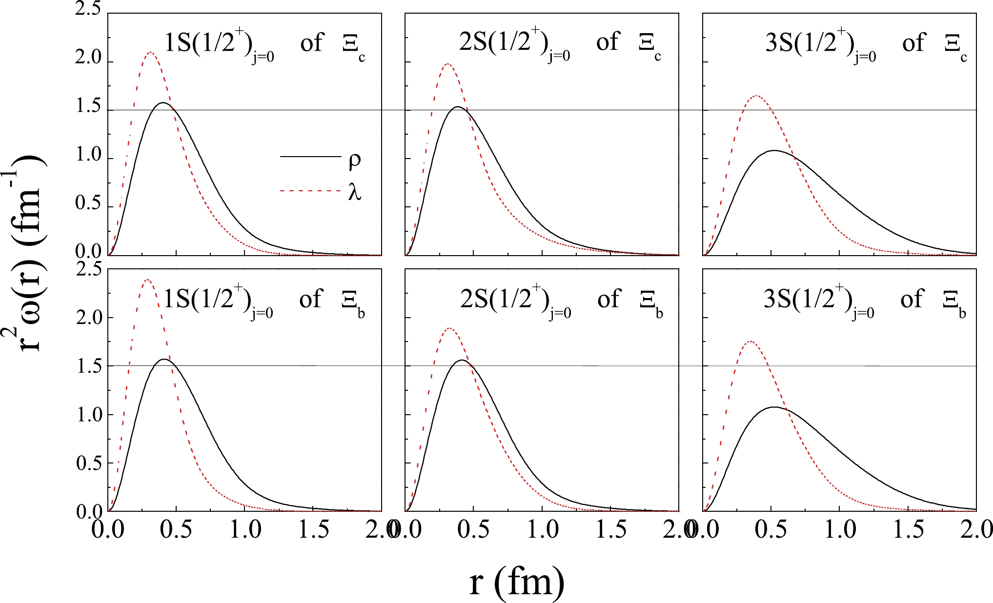
Figure 7. (color online) Radial probability density distributions for some
$ nS $ states in the$ \Xi_{c} $ and$ \Xi_{b} $ families.(1) For the same n states, when L changes from 1 to 4, their
$ \langle r_{\rho}^{2}\rangle ^{1/2} $ values increase slightly. However, their$ \langle r_{\lambda}^{2}\rangle ^{1/2} $ values gradually increase. A similar phenomenon is observed in Figs. 5 and 6, where the radial probability of$ r_{\rho}^{2}\omega(r_{\rho}) $ changes slightly with different L values. However, the peak value of$ r_{\lambda}^{2}\omega(r_{\lambda}) $ significantly shifts outward with increasing L.(2) For the same L states,
$ \langle r_{\rho}^{2}\rangle ^{1/2} $ and$ \langle r_{\lambda}^{2}\rangle ^{1/2} $ generally increase with increasing n. The peaks of their probability densities in general shift outward, as shown in Fig. 7.(3) The shapes of the eight black (solid) lines in Fig. 5 are almost the same as those in Fig. 6. The values of
$ \langle r_{\rho}^{2}\rangle ^{1/2} $ for the same state are almost the same for the$ \Xi_{c} $ ($ \Xi_{c}^{'} $ ) and$ \Xi_{b} $ ($ \Xi_{b}^{'} $ ) families. This reflects the fact that the configurations of the two light quarks in the$ \Xi_{c} $ ($ \Xi_{c}^{'} $ ) and$ \Xi_{b} $ ($ \Xi_{b}^{'} $ ) baryons are similar to each other.(4) As shown in Tables 1−6, the root mean square radii of those baryons that have been experimentally well established are generally less than 0.8 fm.
As the root mean square radius increases, the radial probability distribution of the wave function becomes more outwardly extended, and baryons become looser. In general, the root mean square radius of a compact baryon is within a threshold, which is helpful for estimating the upper limit of the corresponding mass spectrum and for constraining the number of members in each heavy baryon family.
-
Regge trajectories is an effective method for describing hadron mass spectra [122−126]. In 2011, Ebert
$ et\ al. $ constructed the heavy baryon Regge trajectories for both the$ (J, M^{2}) $ and$ (n, M^{2}) $ planes [52].In this subsection, we investigate the Regge trajectories in the
$ (J, M^{2}) $ plane based on our calculated mass spectra. The states in a baryon family can be classified according to the following parities and angular momenta: (1) natural$ P=(-1)^{J+1/2} $ and unnatural$ P=(-1)^{J-1/2} $ parities (written in short as$ NP $ and$ UP $ , respectively) [127]; (2)$ J=j+1/2 $ and$ J=j-1/2 $ (written in short as$ NJ $ and$ UJ $ ). Thus, the states in the$ \Xi_{c} $ or$ \Xi_{b} $ family are divided into two groups, and the states in the$ \Xi_{c}^{'} $ or$ \Xi_{b}^{'} $ family are divided into six groups. In this paper, we use the following definition for the$ (J, M^{2}) $ Regge trajectories:$ \begin{eqnarray} M^{2}=\alpha J+ \beta, \end{eqnarray} $

(33) where α and β are the slope and intercept. In Figs. 8 and 9, we plot the Regge trajectories in the
$ (J, M^{2}) $ plane. The three lines in each figure correspond to the radial quantum numbers n = 1, 2, 3, respectively. The fitted slopes and intercepts of the Regge trajectories are listed in Tables 7 and 8.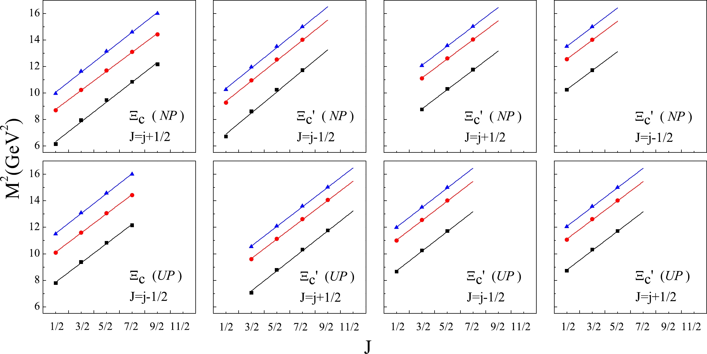
Figure 8. (color online)
$ (J, M^{2}) $ Regge trajectories for the$ \Xi_{c} $ ($ \Xi_{c}^{'} $ ) families, with$ M^{2} $ in GeV$ ^{2} $ .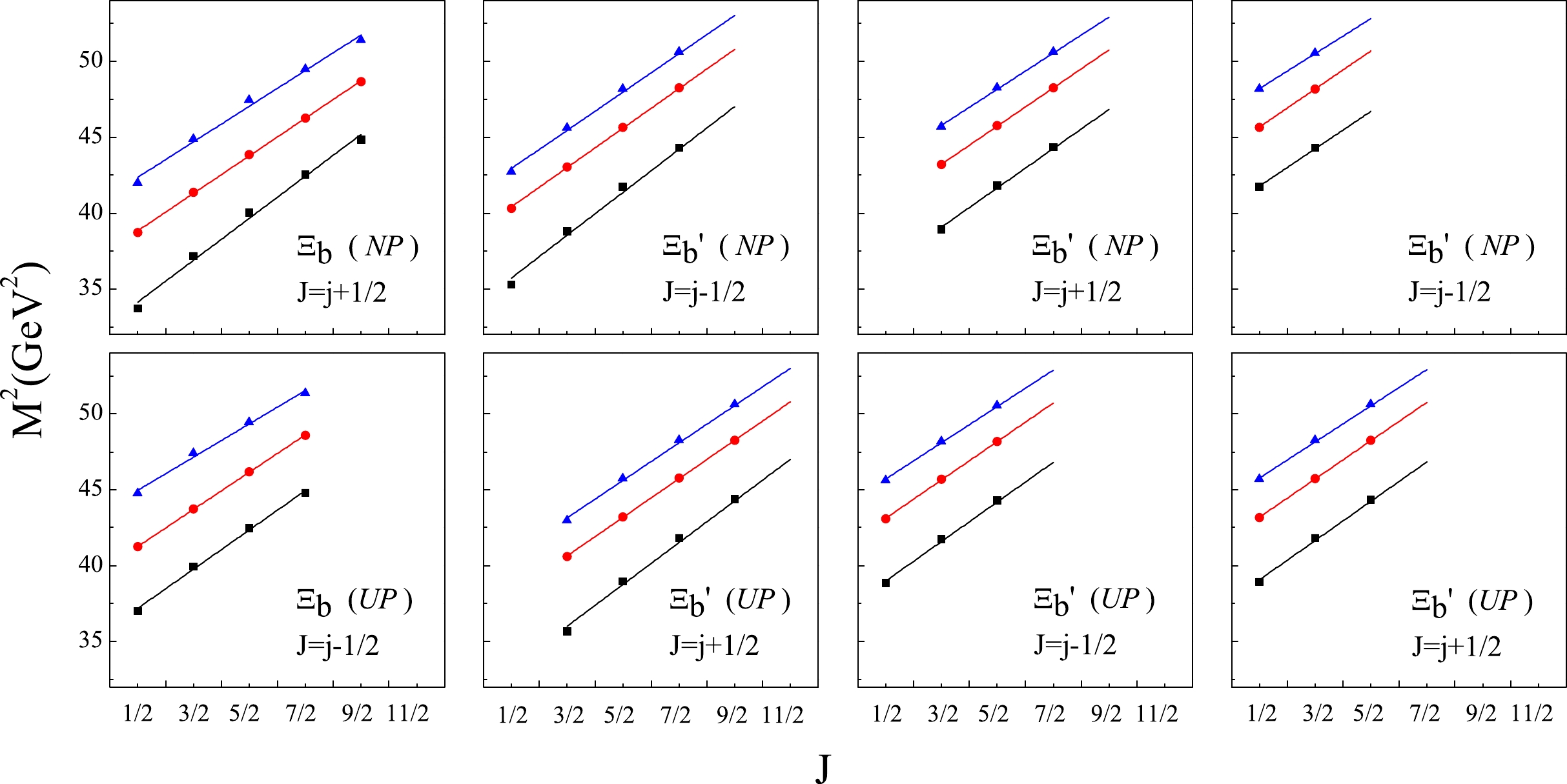
Figure 9. (color online)
$ (J, M^{2}) $ Regge trajectories for the$ \Xi_{b} $ ($ \Xi_{b}^{'} $ ) families, with$ M^{2} $ in GeV$ ^{2} $ .Trajectory $n=1$ 

$n=2$ 

$n=3$ 

α/GeV2 β/GeV2 α/GeV2 β/GeV2 α/GeV2 β/GeV2 $\bar{3}_{F}(NP)(NJ)$ 

$1.493\pm0.056$ 

$5.580\pm0.160$ 

$ 1.433\pm0.022 $ 

$8.047\pm0.063$ 

$ 1.507\pm0.032 $ 

$9.305\pm0.091$ 

$\bar{3}_{F}(UP)(UJ)$ 

$1.456\pm0.043$ 

$7.122\pm0.098$ 

$ 1.446\pm0.023$ 

$9.399\pm0.052$ 

$ 1.501\pm0.026$ 

$10.784\pm0.059$ 

$6_{F}(NP)(UJ)$ 

$1.592\pm0.058$ 

$6.098\pm0.166$ 

$1.530\pm0.033$ 

$8.611\pm0.096$ 

$1.539\pm0.031$ 

$9.574\pm0.089$ 

$6_{F}(UP)(UJ) $ 

$1.487\pm0.033$ 

$7.959\pm0.076$ 

$1.473\pm0.026$ 

$10.292\pm0.059$ 

$1.482\pm0.018$ 

$11.260\pm0.041$ 

$6_{F}(NP)(UJ) $ 

$1.433\pm0.026$ 

$9.545\pm0.044$ 

$1.433\pm0.026$ 

$11.837\pm0.045$ 

$1.453\pm0.015$ 

$12.795\pm0.026$ 

$6_{F}(UP)(NJ) $ 

$1.507\pm0.040$ 

$4.933\pm0.153$ 

$1.459\pm0.022$ 

$7.451\pm0.082$ 

$1.474\pm0.019$ 

$8.371\pm0.071$ 

$6_{F}(NP)(NJ) $ 

$1.455\pm0.031$ 

$6.618\pm0.098$ 

$1.437\pm0.025$ 

$8.980\pm0.079$ 

$1.454\pm0.018$ 

$9.911\pm0.058$ 

$6_{F}(UP)(NJ) $ 

$1.463\pm0.034$ 

$8.041\pm0.078$ 

$1.444\pm0.025$ 

$10.383\pm0.057$ 

$1.460\pm0.019$ 

$11.336\pm0.043$ 

Table 7. Fitted values for the slope and intercept of the Regge trajectories for the
$\Xi_{c}$ and$\Xi_{c}^{'}$ families.Trajectory $n=1$ 

$n=2$ 

$n=3$ 

α/GeV2 β/GeV2 α/GeV2 β/GeV2 α/GeV2 β/GeV2 $\bar{3}_{F}(NP)(NJ)$ 

$2.760\pm0.134$ 

$32.756\pm0.386$ 

$2.470\pm0.027 $ 

$37.595\pm0.077$ 

$2.341\pm0.122$ 

$41.187\pm0.350$ 

$\bar{3}_{F}(UP)(UJ)$ 

$2.582\pm0.099$ 

$35.891\pm0.226$ 

$2.449\pm0.014$ 

$40.029\pm0.033$ 

$ 2.190\pm0.114$ 

$43.86\pm0.262$ 

$6_{F}(NP)(UJ)$ 

$2.820\pm0.129$ 

$34.316\pm0.371$ 

$2.592\pm0.032$ 

$39.116\pm0.092$ 

$2.518\pm0.076$ 

$41.681\pm0.219$ 

$6_{F}(UP)(UJ) $ 

$2.605\pm0.087$ 

$37.677\pm0.199$ 

$2.529\pm0.014$ 

$41.849\pm0.033$ 

$2.388\pm0.051$ 

$44.509\pm0.116$ 

$6_{F}(NP)(UJ) $ 

$2.465\pm0.068$ 

$40.538\pm0.117$ 

$2.512\pm0.013$ 

$44.409\pm0.022$ 

$2.309\pm0.038$ 

$47.045\pm0.065$ 

$6_{F}(UP)(NJ) $ 

$2.747\pm0.113$ 

$31.888\pm0.428$ 

$2.536\pm0.019$ 

$36.834\pm0.072$ 

$2.462\pm0.062$ 

$39.454\pm0.235$ 

$6_{F}(NP)(NJ) $ 

$2.580\pm0.085$ 

$35.207\pm0.273$ 

$2.510\pm0.016$ 

$39.450\pm0.050$ 

$2.374\pm0.053$ 

$42.222\pm0.170$ 

$6_{F}(UP)(NJ) $ 

$2.588\pm0.089$ 

$37.766\pm0.205$ 

$2.522\pm0.018$ 

$41.921\pm0.041$ 

$2.382\pm0.057$ 

$44.573\pm0.131$ 

Table 8. Fitted values for the slope and intercept of the Regge trajectories for the
$\Xi_{b}$ and$\Xi_{b}^{'}$ families.Linear trajectories appear clearly in the
$ (J, M^{2}) $ plane. All the data points fall on the trajectory lines. This indicates that the Regge trajectory is strongly universal, and our theoretical calculations are reliable. These trajectories are almost parallel but not equidistant, which is an apparent difference between our mass spectra and those in Ref. [52].In this paper, we do not show the Regge trajectories in the
$ (n, M^{2}) $ plane. In fact, linear trajectories in the$ (n, M^{2}) $ plane can not be constructed from our predicted masses. As will be mentioned in subsection III.E, if the observation of heavy baryons in forthcoming experiments touches the$ 3S $ sub shell, it will allow to check the$ (n, M^{2}) $ Regge trajectories, which in turn will allow to determine whether a single heavy baryon is a three-quark system or a quark-diquark system. -
For the well determined
$ \Xi_{c} $ ($ \Xi^{'}_{c} $ ) baryons in the PDG, we can assign them to the corresponding positions as follows:$ \Xi_{c}^{+} $ and$ \Xi_{c}^{0} \leftrightarrow \Xi_{c} 1S(\frac{1}{2}^{+}) $ ,$ \Xi_{c}^{'+,0} \leftrightarrow \Xi_{c} 1S(\frac{1}{2}^{+}) $ ,$\Xi_{c}(2645)^{+,0} \leftrightarrow \Xi_{c}^{'} 1S(\frac{3}{2}^{+})$ , and$ \Xi_{c}(2790)^{+,0} $ and$\Xi_{c}(2815)^{+,0} \leftrightarrow \Xi_{c} 1P(\frac{1}{2}^{-},\frac{3}{2}^{-})$ , as listed in Tables 1 and 2. The measured masses are well reproduced in our calculations, and the deviation is usually below 14 MeV. In addition, it should be noted that$ \Xi_{c}(2645) $ in the PDG should be labelled with$ \Xi_{c}^{'}(2645) $ .$ \Xi_{c}(2970) $ , previously known as$ \Xi_{c}(2980) $ , was first observed by Belle in 2006 [29]. The quantum numbers of$ \Xi_{c}(2970) $ were determined as$ \frac{1}{2}^{+} $ in the latest PDG. In our calculations, the only candidate was$ 2S(\frac{1}{2}^{+}) $ of$ \Xi_{c} $ , as shown in Table 1. The predicted mass was 15 MeV less than the experimental result. Finally,$ \Xi_{c} $ (3055) and$ \Xi_{c} $ (3080) were observed by BABAR [4] and Belle [ 10, 15]. As shown in the PDG, their spin and parity values have not yet been elucidated. According to the measured masses,$ \Xi_{c} $ (3055) and$ \Xi_{c} $ (3080) were likely the$ 1D $ doublet ($ \frac{3}{2}^{+} $ ,$ \frac{5}{2}^{+} $ ) of$ \Xi_{c} $ in Table 1 or the$ 2S $ doublet ($ \frac{1}{2}^{+} $ ,$ \frac{3}{2}^{+} $ ) of$ \Xi_{c}^{'} $ in Table 2. Considering that the system with a smaller root mean square radius (especially for$ \langle r_{\lambda}^{2}\rangle ^{1/2} $ ) was more stable, the$ 2S $ doublet states should be the ideal candidates.Outside of the PDG data, Belle and the LHCb observed four charm-strange baryons, namely
$ \Xi_{c}(2930) $ [12],$ \Xi_{c}(2923) $ ,$ \Xi_{c}(2939) $ , and$ \Xi_{c}(2964) $ [13], whose masses were very close to each other. By the predicted masses in Tables 1 and 2, the above four baryons can be assigned to be the first orbital ($ 1P $ ) excitation of$ \Xi_{c}^{'} $ . At present, we can not determine their quantum numbers accurately.$ \Xi_{c} $ (3123) was observed by the BABAR Collaboration [4]. However, it has not yet appeared in the PDG [28]. In our calculations, the predicted masses of$ \Xi_{c} 3S(\frac{1}{2}^{+}) $ and$ \Xi_{c}^{'} 2S(\frac{3}{2}^{+}) $ were 3155 MeV and 3095 MeV, respectively, relatively closer to the measured value of$ \Xi_{c} $ (3123) than those of other states. Because$ \Xi_{c}^{'} 2S(\frac{3}{2}^{+}) $ has been considered as the candidate of$ \Xi_{c}(3080) $ ,$ \Xi_{c} $ (3123) is likely the$ \Xi_{c} 3S(\frac{1}{2}^{+}) $ state. Of course, whether$ \Xi_{c} $ (3123) exists remains to be tested.The calculated mass spectra of
$ \Xi_{b} $ and$ \Xi^{'}_{b} $ families are listed in Tables 4−6 where overall six bottom-strange baryons with determined quantum numbers in the PDG have been assigned to the possible states, such as$ \Xi_{b}^{-,0} \leftrightarrow \Xi_{b} 1S(\frac{1}{2}^{+}) $ ,$ \Xi_{b}^{'}(5935)^{-} \leftrightarrow \Xi_{b}^{'} 1S(\frac{1}{2}^{+}) $ , and$ \Xi_{b}(5945)^{0} $ and$ \Xi_{b}(5955)^{-} \leftrightarrow \Xi_{b}^{'} 1S(\frac{3}{2}^{+}) $ .In 2021, the AMS collaboration determined
$ \Xi_{b}(6100) $ with the quantum numbers$ J^{P}=\frac{3}{2}^{-} $ by measuring the typical decay chain of$ \Xi_{b}(6100)^{-}\rightarrow \Xi_{b}^{*0}\pi^{-}\rightarrow \Xi_{b}^{-}\pi^{+}\pi^{-} $ [24]. Very recently, the values of$ J^{P}=\frac{3}{2}^{-} $ of$ \Xi_{b}(6100) $ were written into the PDG data. Table 4 shows that the mass of$ \Xi_{b}(6100) $ is very close to that of the$ \Xi_{b} 1P(\frac{3}{2}^{-}) $ state. Therefore,$ \Xi_{b}(6100) $ is most likely the$ 1P(\frac{3}{2}^{-}) $ state of$ \Xi_{b} $ . From Tables 4 and 5, we find that the experimental data can be well reproduced by our theoretical calculations. In addition, it should be pointed out that$ \Xi_{b}(5945)^{0} $ and$ \Xi_{b}(5955)^{-} $ in the PDG ought to be labelled with$ \Xi_{b}^{'}(5945)^{0} $ and$ \Xi_{b}^{'}(5955)^{-} $ .The last two
$ \Xi_{b} $ baryons in the PDG,$ \Xi_{b}(6227)^{-} $ and$ \Xi_{b}(6227)^{0} $ , were reported by the LHCb Collaboration in 2018 [23]. However, their spin and parity values are still not confirmed. In Tables 4 and 5, there are six states (one$ 2S $ state of$ \Xi_{b} $ and five$ 1P $ states of$ \Xi_{b}^{'} $ ) whose masses range from 6224 MeV to 6243 MeV. Each of them could be considered as a possible assignment to$ \Xi_{b}(6227) $ .In 2021, two bottom-strange baryons
$ \Xi_{b}(6327) $ and$ \Xi_{b}(6333) $ were reported by the LHCb Collaboration. Very recently, the LHCb implied in experiment that they should belong to the$ \Xi_{b} $ 1D($ \frac{3}{2}^{+} $ ,$ \frac{5}{2}^{+} $ ) doublet [25]. In Table 4, one can see that the predicted masses of the 1D doublet ($ \frac{3}{2}^{+} $ ,$ \frac{5}{2}^{+} $ ) of$ \Xi_{b} $ indeed match with the experimental data of$ \Xi_{b}(6327) $ and$ \Xi_{b}(6333) $ . -
The shell structures of the mass spectra are shown in Figs. 10 and 11, where only the states with their root mean square radii less than 1 fm were collected. In these two figures, the well established baryons in the experiment were labeled next to the corresponding states, and for the recently observed baryons, their possible positions were arranged preliminarily according to the discussions in subsection III.D.
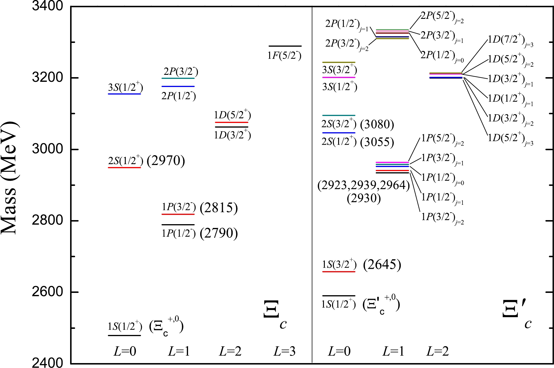
Figure 10. (color online) Mass spectrum shells of the
$ \Xi_{c} $ and$ \Xi_{c}^{'} $ families.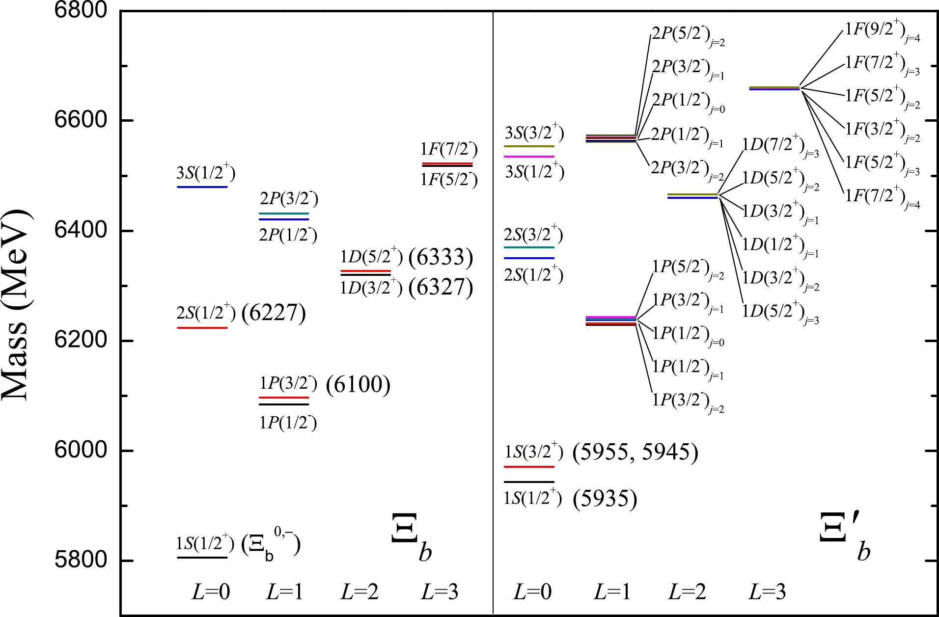
Figure 11. (color online) Mass spectrum shells of the
$ \Xi_{b} $ and$ \Xi_{b}^{'} $ families.From these two figures, we obtain a bird's-eye view of the mass spectra. Firstly, the baryon spectra of
$ \Xi_{c} $ ($ \Xi_{c}^{'} $ ) and$ \Xi_{b} $ ($ \Xi_{b}^{'} $ ) have almost the same shell structures. Secondly, the baryons with lighter masses were discovered earlier in experiments. Thirdly, there is a serious energy degeneracy in the P, D and F states for the$ \Xi_{c}^{'} $ ($ \Xi_{b}^{'} $ ) family. In addition, the calculated masses for the$ 2S $ states of the$ \Xi_{c} $ ($ \Xi_{b} $ ) family are very close to those of the$ 1P $ states of the$ \Xi_{c}^{'} $ ($ \Xi_{b}^{'} $ ) family. This makes these states hard to be identified in experiments.Finally, the states that can be possibly observed experimentally can be predicted. For the
$ \Xi_{c} $ family, the$ 1D $ doublets and the$ 3S(1/2)^{+} $ are likely to be experimentally observed first. With respect to the$ \Xi_{c}^{'} $ family, the$ 3S $ doublets might be the next ones to be observed. However, the predicted mass range of the$ 3S $ doublet states overlaps heavily with that of the$ 1D $ states. As to the$ \Xi_{b} $ family, we find that the$ 1P(1/2)^{-} $ state should have been discovered earlier in experiments and the predicted mass would be$ 6084 $ MeV. The possibly observed states in the$ \Xi_{b}^{'} $ family should be the$ 1P $ states where experimental observations will encounter the difficulty of an energy degeneracy. -
Motivated by the experimental developments associated with single heavy baryons, we investigated the strange single heavy baryon spectra in a three-quark system, where the relativistic quark model and the ISG method were employed. Considering that the λ-mode appears lower in terms of the energy for definite states
$ nL(J^{P}) $ , we only focused on the λ-mode and obtained the mass spectra of the$ \Xi_{c} $ ,$ \Xi_{c}^{'} $ ,$ \Xi_{b} $ , and$ \Xi_{b}^{'} $ families. For the well established baryons, our predicted masses reproduced existing experimental data accurately. We also investigated the root mean square radii and the radial probability density distributions, from which we learned more about the structure of strange single heavy baryons.Based on the predicted mass spectra, we constructed the Regge trajectories in the
$ (J,M^{2}) $ plane. Nevertheless, we could not construct linear trajectories in the$ (n,M^{2}) $ plane, which is an apparent difference between our mass spectra and those in the relativistic quark-diquark picture [52].For some recently observed baryons, we preliminarily determined their reasonable positions in the mass spectra. Finally, the mass spectral structures of the
$ \Xi_{c} $ ($ \Xi_{c}^{'} $ ) and$ \Xi_{b} $ ($ \Xi_{b}^{'} $ ) families were presented, from which we obtained a bird's-eye view of the mass spectra and were able to easily foresee the experimental course. Then, we analyzed some states that might be observed in the forthcoming experiments. -
Zhen-yu Li, one of the authors, thanks Wen-chao Dong for his valuable reference, helpful discussion, and kind help in programming. Li is also grateful to Professor Xian-Jian Shi for his encouragement. The authors would like to thank the editors for polishing and typesetting this article.
APPENDIX
Systematic analysis of strange single heavy baryons ${ \boldsymbol\Xi_{\boldsymbol c} }$ and ${\boldsymbol\Xi_{\boldsymbol b} }$
- Received Date: 2023-03-15
- Available Online: 2023-07-15
Abstract: Motivated by the experimental progress in the study of heavy baryons, we investigate the mass spectra of strange single heavy baryons in the λ-mode, using the relativistic quark model and the infinitesimally shifted Gaussian basis function method. We show that experimental results are well captured using the predicted masses. The root mean square radii and radial probability density distributions of the wave functions are analyzed in detail. Meanwhile, the mass spectra allow us to successfully construct the Regge trajectories in the


 DownLoad: