


 Abstract
 HTML
HTML Reference
 Related
 PDF
PDF


-
White dwarfs (hereafter WDs) are usually made up of C+O. However, it is also possible for their cores to be hot enough to burn carbon but not hot enough to burn Ne, forming a WD with a core of O+Ne+Mg. At the later stage of WDs, the star ejects large quantities of matter. After great mass loss, if the remaining core mass is less than 1.44 solar masses, the star may evolve into a WD.
WDs form at very high temperatures. Because they have no source of energy, they will therefore gradually give off heat and cool down, whereupon its radiation will decrease over time from its initial high color temperature to red. This surface temperature is defined in astronomy as the effective temperature
$ T_{\rm{eff}} $ as per Stefan's law, so that$ \begin{array}{*{20}{l}} L_{\rm{rad}}=4\pi R^2\sigma T^4_{\rm{eff}}, \end{array} $

(1) where R the radius of the star,
$ L_{\rm{rad}} $ is the radiation luminosity, and$ \sigma=5.6704\times10^{-5}\rm{erg s^{-1}cm^{-2}K^{-4}} $ is the radiation constant from Stefan's law.$ T_{\rm{eff}} $ is a measure of the energy flux at the surface and not a real temperature, but it nevertheless constitutes a useful measure of the atmospheric temperature of the star.As is well known, the effective temperature of WDs is mostly in the range 5500–40000 K, while a few are outside this range, and the internal temperature of WDs is on the order of
$ \sim10^6-10^7 $ K, with a total thermal energy less than$ 10^{47} $ ergs. Mestel. [1] discussed the energy sources of WDs. Avakian. [2] also studied the configurations of hot WDs with nuclear sources of energy. Bildsten & Hall. [3] discussed the sources of white dwarfs, suggesting that there are small amounts of$ ^{22} $ Ne in some WDs that may constitute an extra source of heat in carbon-oxygen WDs. Single-particle$ ^{22} $ Ne sedimentation may be considered a possible heat source [4, 5]. However, some work suggests that$ ^{22} $ Ne must separate into clusters, enhancing diffusion, in order for sedimentation to provide heating on the observed timescale. Recently, the sources of ultra-high-energy photons for WD pulsars have been discussed by Lobato et al. [6]. Cheng et al. [7] discuss the cooling anomaly of high-mass WDs, pointing out that$ ^{22} $ Ne settling in C/O-core WDs could account for this extra cooling delay. Caplan et al. [8] studied this topic using molecular dynamics methods and phase diagrams, from which they ruled out the isotope$ ^{22} $ Ne as a possible cause of the extra heating. Therefore, the problem of additional heat sources for WDs remains a challenging topic.In this paper, we selected 13 red giant branch (RGB) stars to present a new model of the number of magnetic monopoles (hereafter MMs) captured, and seek to solve the energy source problem for WDs based on MM catalytic nuclear decay
(the Rubakov-Callan (RC) effect) [9, 10]. MMs are hypothetical magnetic particles with a single north or south magnetic pole, which have been proposed in string theory. Research on MMs has long been a hot topic among physicists and astronomers. Some papers have discussed the issues of MMs, (e.g., Callan [9], Detrixhe et al. [11], Frank et al. [12], Fujii & Pierre [13], Kain [14], Rajantie [15]). Recently, Mavromatos & Mitsou. [16] discussed the developments in both theory and experimental searches for MMs in past, current, and future colliders and in the cosmos. We also are interested in the problem of MMs and other related issues ((e.g., Liu. [17, 18], Liu & Gu [19], Liu et al. [20], Liu [21−26], Peng et al. [27, 28]). The arrangement of this paper is as follows. In the next section, we discuss the number of possible magnetic monopoles in space and the luminosity due to the RC effect by MMs. In Section III, we describe our models and the luminosity function due to magnetic monopole catalytic nuclear decay. In Section IV, some results and discussions are presented. Finally, our conclusions are summarized in Section V.
-
According to some research, the interaction of MMs with neutral hydrogen atoms is very weak. Therefore, during the process of formation of celestial bodies, very few MMs are captured in the collapse of a neutral hydrogen cloud and collect in the core of a star or planet. MMs typically may be contained within stars and planets, and they are mostly captured from space during their lifetime after formation. One type of interaction that MMs undergo in stars and planets might be the RC effect, through which MMs may catalyze nucleon decay, as expressed by
$p+M\rightarrow e^+\pi^0+ M+ {\rm debris}$ (x%) and$p+M\rightarrow e^+ \mu^{\pm} + M+ {\rm debris}$ (y%). The ratio of the cross sections of the above reactions$ x/y $ may be a few percent, which is on the order of$ \sim10^{-4} $ [10]. Bernreuther and Craigie [29] discussed the cross section of monopole-induced proton decay in SU(5) for the above reactions, showing that the ratio of cross sections of the above reactions$ x/y $ may be$ (2.5\sim2.8)\times10^{-4}/(0.1\sim0.3) $ .The number (flow) of MMs captured in space at the surface of stars and planets (including earth) is estimated as follows [30]:
$ N_{m}=4\pi^2 R^2\eta\phi t\left[1+\left(\frac{v_{\rm{esc}}}{v_m}\right)^2\right], $

(2) where ϕ is the flux of MMs intercepted in space and
$ v_{\rm{esc}}=(2GM/R)^{1/2} $ , t are the escape velocity from the star and cooling age of the star, respectively.$ v_m $ represents the velocity of MMs in space, For a planet,$ \dfrac{v_{\rm{esc}}}{v_m}\ll1 $ , and$ \dfrac{v_{\rm{esc}}}{v_m}\approx1 $ for ordinary stars, but$ \dfrac{v_{\rm{esc}}}{v_m}\gg1 $ for compact objects such as WDs, neutron stars, galactic nuclei, and quasars. Therefore, the ratio between the number of MMs captured and the number of nuclei in the MMs accumulation area is [30]$ \frac{N_m}{N_B}=5.10\times10^{-34}\eta R^2_\ast\left(\frac{t_9}{M_\ast}\right)\left(\frac{\phi}{\phi_0}\right)\left[1+4.256v^{-2}_{-3}\left(\frac{M_\ast}{R_\ast}\right)\right], $

(3) where
$ R_\ast=R/R_{\odot} $ ,$ M_\ast=M/M_{\odot} $ ,$ v_{-3}=v_m/10^{-3}c $ ,$ t_{9}=t/10^9 $ Yr, and c is the speed of light.$ \phi_0\approx 10^{-12} \rm{cm^{-2}s^{-1}Sr^{-1}} $ [31]. η is the probability of the capture of MMs by stars, which depends on the ratio of the penetration distance$ l_{\rm{pd}} $ of an MM in a star to the star's radius. In general, we have$ l_{\rm{pd}}\approx1.2\times10^{30}v_{-3}n_e^{-1}T_e^{1/2} $ for plasma [30]. For example, with$n_e\sim10^{22} {\rm cm^{-3}}, T_e\sim10^6$ K for the sun, we have$ l_{\rm{pd}}\sim10^{11}, \eta\sim0.7 $ ; however, for WDs and neutron stars,$ n_e\geq10^{30}, n_e\geq10^{35}\rm{cm^{-3}} $ , respectively, and$ \eta\sim1 $ . For quasars and active galactic nuclei,$ M_\ast\sim10^8, T_e\sim10^5 $ K,$ \eta\sim1 $ .The velocity of MMs is also determined as a function of monopole mass by
$ \beta_{\rm{T}} $ as follows [32].$ \begin{array}{*{20}{l}} v_m=c\beta_{\rm{T}}=\left\lbrace \begin{array}{ll}\; 3\times10^{-3}c\left(\dfrac{10^{16}\rm{GeV}}{m}\right)^{0.5}\; \; ( m<10^{17}\rm{GeV})\\ \; 10^{-3}c \; \; \; \; \; \; \; \; \; \; \; \; \; \; \; \; \; \; \; (\rm{otherwise}). \end{array} \right. \end{array} $

(4) According to Eq. (3), for WDs we have
$ \eta\sim1 $ ; thus, the total number of magnetic monopoles trapped in space after the formation of stars (or planets) is estimated to be$ N_{m}=7.18\times10^{11}n_{\rm{B}}R^5_\ast\phi\left(\frac{t_9}{M_\ast}\right)\left[1+4.256v^{-2}_{-3}\left(\frac{M_\ast}{R_\ast}\right)\right]. $

(5) For astronomy, the most important property of a magnetic monopole is that it can trigger the RC effect, as independently proposed by Rubakov and Callen [9, 10]. The reaction cross section is about
$ \sigma_m\approx10^{-25}\sim10^{-26}\rm{cm}^2 $ , almost reaching the Thomson cross section ($6.665\times 10^{-25}\rm{cm}^2$ ). The luminosity of various types of celestial bodiesdue to the RC effect (i.e., RC luminosity) can be estimated as follows. In the core area, where the magnetic monopole is concentrated, the nuclear decay reaction is catalyzed by the magnetic monopoles and the total luminosity produced is [30]$ L_m\approx\frac{4\pi}{3}r_c^3n_mn_{\rm{B}}\langle\sigma_m v_{\rm{T}}\rangle m_{\rm{B}}c^2=N_m n_{\rm B}\langle\sigma_m v_{\rm{T}}\rangle m_{\rm{B}}c^2, $

(6) where
$ r_c $ , and$n_m, n_{\rm B}$ are the radius of the stellar central region and the number densities of MMs and nucleons, respectively.In Eq. (6),
$ v_{\rm{T}} $ is the thermal movement speed of the nucleus relative to the magnetic monopole. We will ignore the thermal velocity of the magnetic monopole due to its great mass. We thus only consider the contributions from the thermal velocity of the nucleus. According to$1/2mv_{\rm T}^2=3/2kT$ , we have$v_{\rm{T}}=\sqrt{3kT/m_B} \approx 1.5745\times 10^{7}T_6^{1/2}$ cm/s, where T is the temperature,$ T_6=T/10^6 $ K,$ k=1.38\times10^{-16}\rm{erg/s} $ is the Boltzmann constant, and$m_{\rm B}\approx1.67\times10^{-24}$ g is the nucleon mass. As the central temperature of WDs is about$ \sim10^6 $ K, we have$ v_T\sim10^{-3}c $ .As a general rule, the reaction cross section of the RC effect
$ \sigma_m $ is$10^{-26}\sim10^{-24}\;\rm{cm}^2$ . Ma & Tang [33] gave a value$ \sigma_m\approx4.28676\times10^{-24}\rm{cm}^2 $ for the cross section of the proton with different channels using SU(5) grand unification theory. In the RC process, MMs induced nucleon decay, followed by nucleon decay into$ \pi^0 $ mesons,$ \mu^\pm $ leptons, and positrons$ e^+ $ , and$ \mu^\pm $ and$ \pi^0 $ again decay into photons and electron-positron pairs$ e^\pm $ . The positrons then undergo annihilation with electrons to form photons. The net effect is that the rest mass energy of nucleons ($ m_{\rm{B}}c^2 $ ) is entirely converted to radiant energy with 100% efficiency ($ 1m_{\rm{B}}c^2\approx1\rm{GeV}\approx1.6\times10^{-3}\rm{ergs} $ ). -
It is well known that WDs evolve from red giants with mass less than
$ 8M_{\odot} $ . The MM content of the trapping accumulation set is mainly from the red giant branch (RGB) phase. The$ M_{\ast} $ and$ R_{\ast} $ for RGB stars is given by [34, 35]$ M^{\rm{r}}_{\ast}=\frac{M_{\rm{RG}}}{M_\odot}=\left(\frac{\nu_{\rm{max}}}{\nu_{\rm{max},\odot}}\right)^3\left(\frac{\Delta\nu}{f_{\Delta\nu}\Delta\nu_{\odot}}\right)^{-4}\left(\frac{T_{\rm{eff}}}{T_{\rm{eff},\odot}}\right)^{1.5}, $

(7) $ R^{\rm{r}}_{\ast}=\frac{R_{\rm{RG}}}{R_\odot}=\left(\frac{\nu_{\rm{max}}}{\nu_{\rm{max},\odot}}\right)\left(\frac{\Delta\nu}{f_{\Delta\nu}\Delta\nu_{\odot}}\right)^{-2}\left(\frac{T_{\rm{eff}}}{T_{\rm{eff},\odot}}\right)^{0.5}, $

(8) where
$ \nu_{\rm{max},\odot}=3090\mu $ Hz,$ \Delta\nu_{\odot}=135.1\mu $ Hz,$ T_{\rm{eff},\odot}=5777 $ K, and$ \Delta\nu\simeq \alpha(\nu_{\rm{max}/\mu{\rm{Hz}}})^{\beta} $ (here$\alpha=0.268\mu$ Hz,$ \beta=0.758 $ )[36].$ f_{\Delta\nu} $ is a typical asteroseismic correction factor, which is between 0.98 and 1.02 [37]. The predicted$ \nu_{\rm{max}} $ values are calculated using the scaling relation [38]$ \frac{\nu_{\rm{max}}}{\nu_{\rm{max}\odot}}=\left(\frac{g}{g_{\odot}}\right)\left(\frac{T_{\rm{eff}}}{T_{\rm{eff},\odot}}\right)^{-0.5}. $

(9) where g is the surface gravity of the star and
$ g_\odot=27487\;\rm{cm/s^2} $ . -
According to Eqs. (5)–(9), the number of magnetic monopoles captured from space and the total luminosity due to the RC effect by the MMs are given by
$ N_{m}=7.18\times10^{11}n_{\rm{B}}(R^{r}_\ast)^5\phi\left(\frac{t_9}{M^{r}_\ast}\right)\left[1+4.256v^{-2}_{-3}\left(\frac{M^{r}_\ast}{R^{r}_\ast}\right)\right]. $

(10) $ \begin{aligned}[b] L_m\approx&\frac{4\pi}{3}r_c^3n_mn_{\rm{B}}\langle\sigma_m v_{\rm{T}}\rangle m_{\rm{B}}c^2=N_mn_{\rm B}\langle\sigma_m v_{\rm{T}}\rangle m_{\rm{B}}c^2,\\ =&1.15\times10^{9}n^2_{\rm{B}}(R^{r}_\ast)^5\phi t_9(M^{r}_\ast)^{-1} \\ &\times\langle\sigma_m v_{\rm{T}}\rangle\left[1+4.256v^{-2}_{-3}\left(\frac{M^{r}_\ast}{R^{r}_\ast}\right)\right]. \end{aligned} $

(11) Defining
$ \xi=\phi\langle\sigma_m v_{\rm{T}}\rangle_{-28}=\phi\langle\sigma_m v_{\rm{T}}\rangle/10^{-28} $ , Eq. (11) may be rewritten$ \begin{aligned}[b] L_m\approx&\frac{4\pi}{3}r_c^3n_mn_{\rm{B}}\langle\sigma_m v_{\rm{T}}\rangle m_{\rm{B}}c^2=N_mn_B\langle\sigma_m v_{\rm{T}}\rangle m_{\rm{B}}c^2,\\ =&1.15\times10^{37}n^2_{\rm{B}}(R^{\rm{r}}_\ast)^5t_9(M^{\rm{r}}_\ast)^{-1}\xi\left[1+4.256v^{-2}_{-3}\left(\frac{M^{\rm{r}}_\ast}{R^{\rm{r}}_\ast}\right)\right].\\ \end{aligned} $

(12) From Eqs. (1) and (12), and
$ L_m=L_{\rm{rad}} $ , we obtain$ \xi=5.29\times10^{-15}\sigma M^{r}_\ast t_9^{-1} n^{-2}_{\rm{B}}(R^{r}_\ast)^{-3}T^4_{\rm{eff}}\left[1+4.256v^{-2}_{-3}\left(\frac{M^{r}_\ast}{R^{r}_\ast}\right)\right]^{-1}. $

(13) -
The study of MMs has held considerable interest since MMs were found to be a generic feature of grand unified gauge theories in the physical fields. The theoretical predictions of monopole abundance are problematic in the standard cosmology, as far too many monopoles would have survived annihilation for the universe to have reached its present state. For example, the galactic field that yields the Parker bound is
$ \phi(\sigma v)_{-28}\leq 10^{-16} \rm{cm^{-2}s^{-1}sr^{-1}} $ [39]. Due to MM RC decay, another limit of the flux may be$ \phi(\sigma v)_{-28}\leq10^{-21}\rm{cm^{-2}s^{-1}sr^{-1}} $ [31]. A better-understood limit in WDs may be$ \phi(\sigma v)_{-28}\leq10^{-18} \rm{cm^{-2}s^{-1}sr^{-1}} $ [32]. Then the bound has been stated as$ \phi(\sigma v)_{-28}\leq10^{-28} \;\rm{cm^{-2}s^{-1}sr^{-1}} $ by Freese and Krasteva [40]. In this paper, we study MMs and their numbers in space and discuss our MM model and the luminosity due to RC effect. We select the following typical parameters:$ m=10^{15}, 10^{17} $ GeV,$ \sigma_m=10^{-24}\rm{cm^2} $ ,$\phi=5.59\times10^{-28}, 10^{-26}, 7.59\times 10^{-26}\rm{cm^{-2}s^{-1}sr^{-1}}$ , and$n_{\rm B}=5.99\times10^{31}, 1.89\times 10^{32} \rm{cm^{-3}}$ ,$ t_9=1, 10 $ .Everyone knows that WDs evolve from red giants with mass less than 8 M
$ _\odot $ , we focus on 13 typical RGB stars listed in Tables 1 and 2 [41] and discuss their mass, radius, and cooling age. Depending on an asteroseismic correction factor, we propose five models (I$-$ V) to examine the problem of the energy source of WDs.star TIC ID Gaia ID Gania mag Distance (pc) Galactic substructure Spectral source 1 TIC20897763 Gaia 2365649471033828096 9.41484 457.879 ± 9.435 Gaia Enceladus Sausage APOGEE 2 TIC341816936 Gaia 1421776046335723008 11.623 1547.85 ± 45.63 Gaia Enceladus Sausage APOGEE 3 TIC393961551 Gaia 1506387627917936896 9.57166 500.533 ± 6.312 Gaia Enceladus Sausage APOGEE 4 TIC453888381 Gaia 5230256730347457152 10.9714 788.614 ± 15.999 Halo GALAH 5 TIC279510617 Gaia 5480550450643017216 10.7551 933.263 ± 22.520 Halo GALAH 6 TIC300938910 Gaia 5270675018297844224 10.5629 607.156 ± 7.7075 Halo GALAH 7 TIC198204598 Gaia 1629898685347273856 10.9455 952.885 ± 37.512 Halo ··· 8 TIC1008989 Gaia 3789639280952610304 9.72882 370.56 ± 5.85 Gaia Enceladus Sausage ··· 9 TIC91556382 Gaia 5065009650333147392 10.0855 870.289 ± 34.565 Halo ··· 10 TIC159509702 Gaia 1709195090281718272 12.1542 1595.67 ± 55.605 Halo ··· 11 TIC25079002 Gaia 4669316065700222976 9.91465 716.804 ± 15.5995 Disk APOGEE 12 TIC177242602 Gaia 5262295395367212288 10.1451 532.831 ± 14.294 Disk APOGEE 13 TIC9113677 Gaia 3245485650607651584 10.1791 491.438 ± 10.040 Thick Disk ··· Table 1. Information of the 13 red giant stars selected [41].
star $ \nu_{\rm{max}} $ 

$ \Delta\nu $ /μHz

Teff /K [Fe/H] [α/Fe] 1 61.31383 ± 1.21768 6.81739 ± 0.24990 4988 ± 127 −1.274 ± 0.019 0.219 ± 0.021 2 36.34 ± 0.76 4.2969 ± 0.0715 5068 ± 100 −1.873 ± 0.107 0.248 ± 0.023 3 61.34 ± 1.75 6.68 ± 0.41 5121 ± 105 −1.0751 ± 0.0123 0.156 ± 0.014 4 50.37 ± 1.59 5.953 ± 0.049 4741 ± 100 −0.728 ± 0.07 0.32 ± 0.021 5 28.57 ± 0.16 3.566 ± 0.015 4450 ± 100 −0.49 ± 0.05 0.281 ± 0.017 6 106.30 ± 0.92 9.464 ± 0.131 4908 ± 100 −0.792 ± 0.05 0.2566 ± 0.0165 7 45.86 ± 0.31 5.132 ± 0.032 4979 ± 100 ··· ··· 8 104.33059 ± 1.46618 9.80317 ± 0.15336 4893 ± 100 ··· ··· 9 31.38665 ± 1.03097 4.189 ± 0.186 5192 ± 100 ··· ··· 10 45.37 ± 0.53 5.090 ± 0.027 4724 ± 100 ··· ··· 11 45.238 ± 0.62 4.967 ± 0.121 4797 ± 83 0.1636 ± 0.006 −0.010 ± 0.006 12 54.66 ± 0.33 5.663 ± 0.031 4603 ± 100 −0.1176 ± 0.006 0.125 ± 0.007 13 87.22437 ± 0.87042 8.365 ± 0.198 4764 ± 100 ··· ··· Table 2. Information of the 13 RGB stars [41].
In this paper, we select the asteroseismic correction factors
$ f_{\bigtriangleup\nu}= $ 0.98, 0.99, 1.00, 1.01, 1.02 for our typical models under study, which correspond to models (I$-$ V). Based on Eqs. (8) and (9), we can calculate the mass and the radii of RGB stars$ M^{r}_\ast $ (I$-$ V) and$ R^{r}_\ast $ (I$-$ V) given in Table 3. We determine the stellar (RGB) ages using the packages BASTA [42], isochrones [43], isoclassify [44], PARAM [45, 46], and scaling-giants [47]. These ages correspond to$ t_9 $ (I$ \sim $ V) in Table 4.star $ M_{\ast} $ (I)

$ M_{\ast} $ (II)

$ M_{\ast} $ (III)

$ M_{\ast} $ (IV)

$ M_{\ast} $ (V)

$ R_{\ast} $ (I)

$ R_{\ast} $ (II)

$ R_{\ast} $ (III)

$ R_{\ast} $ (IV)

$ R_{\ast} $ (V)

1 0.8916 0.9286 0.9667 1.0059 1.0464 6.9541 7.0967 7.2408 7.3863 7.5333 2 1.2047 1.2546 1.3061 1.3591 1.4138 10.458 10.672 10.889 11.108 11.329 3 1.0075 1.0493 1.0923 1.1367 1.1824 7.3421 7.4927 7.6449 7.7985 7.9537 4 0.7879 0.8206 0.8542 0.8889 0.9246 7.3045 7.4543 7.6056 7.7585 7.9129 5 1.0154 1.0575 1.1009 1.1456 1.1916 11.186 11.416 11.647 11.882 12.118 6 1.2211 1.2717 1.3239 1.3776 1.4330 6.2057 6.3330 6.4616 6.5914 6.7226 7 1.1587 1.2067 1.2562 1.3072 1.3598 9.1703 9.3584 9.5484 9.7404 9.9342 8 0.9896 1.0404 1.0830 1.1270 1.1723 5.6699 5.7862 5.9037 6.0224 6.1422 9 0.8910 0.9280 0.9660 1.0052 1.0457 9.6193 9.8166 10.016 10.217 10.421 10 0.9221 0.9603 0.9997 1.0403 1.0821 8.5448 8.7201 8.8972 9.0760 9.2566 11 1.1986 1.2483 1.2995 1.3523 1.4066 9.4788 9.6732 9.8696 10.068 10.268 12 1.1762 1.2249 1.2752 1.3270 1.3803 8.6308 8.8078 8.9867 9.1673 9.3497 13 1.0587 1.1026 1.1478 1.1945 1.2425 6.4250 6.5568 6.6899 6.8244 6.9602 Table 3. The mass and radii of the 13 RGB stars selected [41]. The asteroseismic correction factor
$ f_{\bigtriangleup\nu}= $ 0.98, 0.99, 1.00, 1.01, 1.02 defines models I$-$ V, respectively.star scaling-giants Age (Gyr) isochrones Age (Gyr) isoclassify Age (Gyr) PARAM Age (Gyr) BASTA Age (Gyr) $ t_9 $ (I)

$ t_9 $ (II)

$ t_9 $ (III)

$ t_9 $ (IV)

$ t_9 $ (V)

1 5.8 $ \pm $ 3.0

8.77 $ \pm $ 2.9

5.68 $ ^{+0.79}_{-0.83} $ 

9.29 $ ^{+2.82}_{-3.23} $ 

9.0 $ ^{+2.7}_{-2.5} $ 

2 2.9 $ \pm $ 1.8

9.16 $ \pm $ 2.75

7.44 $ ^{+1.36}_{-1.34} $ 

6.52 $ ^{+4.46}_{-3.80} $ 

7.9 $ ^{+2.8}_{-1.9} $ 

3 4.7 $ \pm $ 6.0

5.93 $ \pm $ 3.05

5.63 $ ^{+0.84}_{-0.69} $ 

5.72 $ ^{+4.61}_{-3.14} $ 

7.5 $ ^{+3.3}_{-2.2} $ 

4 10.5 $ \pm $ 3.5

9.72 $ \pm $ 2.50

12.78 $ ^{+0.78}_{-1.59} $ 

11.66 $ ^{+1.50}_{-2.42} $ 

14.8 $ \pm $ 2.8

5 6.4 $ \pm $ 1.1

7.99 $ \pm $ 3.37

10.23 $ ^{+0.95}_{-2.34} $ 

7.68 $ ^{+4.55}_{-4.45} $ 

7.6 $ ^{+0.9}_{-0.8} $ 

6 2.7 $ \pm $ 0.8

3.693 $ \pm $ 0.702

3.34 $ ^{+0.40}_{-0.33} $ 

2.11 $ ^{+0.61}_{-0.49} $ 

2.9 $ ^{+0.6}_{-0.4} $ 

7 3.3 $ \pm $ 0.8

8.749 $ \pm $ 2.16

11.54 $ ^{+0.66}_{-2.83} $ 

1.98 $ ^{+7.13}_{-0.77} $ 

5.8 $ ^{+1.6}_{-1.2} $ 

8 5.8 $ \pm $ 2.0

6.843 $ \pm $ 3.33

6.84 $ ^{+1.50}_{-0.90} $ 

7.27 $ ^{+2.95}_{-2.09} $ 

10.6 $ ^{+3.5}_{-2.9} $ 

9 7.1 $ \pm $ 5.0

6.841 $ \pm $ 3.59

6.43 $ ^{+1.89}_{-0.96} $ 

5.27 $ ^{+2.84}_{-1.77} $ 

8.9 $ ^{+3.8}_{-2.9} $ 

10 4.8 $ \pm $ 1.2

9.344 $ \pm $ 2.331

9.98 $ ^{+1.47}_{-1.18} $ 

7.92 $ ^{+3.47}_{-2.49} $ 

10.0 $ ^{+3.2}_{-2.5} $ 

11 2.1 $ \pm $ 3.2

7.07 $ \pm $ 3.65

1.92 $ ^{+0.17}_{-0.11} $ 

1.84 $ ^{+0.18}_{-0.14} $ 

3.6 $ ^{+0.3}_{-0.4} $ 

12 4.4 $ \pm $ 2.7

7.49 $ \pm $ 3.45

6.54 $ ^{+0.44}_{-0.64} $ 

7.60 $ ^{+4.02}_{-3.74} $ 

6.4 $ ^{+0.6}_{-1.0} $ 

13 5.1 $ \pm $ 2.0

7.07 $ \pm $ 3.65

6.77 $ ^{+1.9}_{-1.35} $ 

8.24 $ ^{+3.24}_{-2.87} $ 

9.7 $ ^{+3.3}_{-2.3} $ 

Based on Eqs. (7)–(9), there are two global seismic parameters, the frequency of maximum power,
$ \nu_{\rm{max}} $ , and the mean large frequency separation,$ \bigtriangleup \nu $ , to describe the oscillations of solar-like stars and radius. The surface gravity and temperature strongly determine the value of the frequency of maximum power, which is given by$ \nu_{\rm{max}}\propto gT^{-0.5}_{\rm{eff}}\propto MR^{-2}T^{-0.5}_{\rm{eff}} $ [48]. On the other hand, the travel time of sound from the center to the surface of a star will directly influence$ \bigtriangleup \nu $ , which is sensitive to the mean stellar density and is given by$ \bigtriangleup \nu\propto \rho^{0.5}\propto M^{0.5}R^{-1.5} $ [49]. In order to reduce systematic errors, by considering the effect on mass, [Fe/H] and$ T_{\rm{eff}} $ interpolation over a grid of models, a modification strategy was adopted by Sharma et al. [37]. Therefore, the asteroseismic correction factor in this paper is selected as$ f_{\bigtriangleup \nu}= $ 0.98, 0.99, 1.00, 1.02, we propose five model (I$-$ V). Detailed information on the mass and radius of RGB stars is shown in Table 3.Based on Eqs. (10) and (12), the age of RGB stars is a key parameter for estimating the number of MMs captured and the luminosity of WDs due to the RC effect by MMs. By combining masses inferred from the asteroseismic parameters with stellar atmospheric parameters and using stellar isochrones, the cooling ages of RGB stars were determined as shown in Table 4 by
$ t_9 $ . Using the packages BASTA [42], isochrones [43], isoclassify [44], PARAM [45, 46], and scaling-giants [47], estimates are obtained of the cooling ages of RGB stars, which are the stellar ages since zero-age main sequence stars are considered.The scaling-giants package accepts asteroseismic parameters, metallicity, and temperature as inputs for model I. In the isochrones, isoclassify, PARAM, and BASTA packages, we take asteroseismic, photometric, and spectroscopic parameters as inputs for models II−V. From the SYD pipeline [50], along with effective temperatures determined through the direct method of isoclassification and metallicity determined by either the APOGEE or GALAH surveys, and using measured seismic
$ \nu_{\rm{max}} $ and$ \bigtriangleup\nu $ values, we can determine the ages with scaling-giants for model I. The SYD pipeline is an automated pipeline to estimate global oscillation parameters, such as the frequency of maximum power ($ \nu_{\rm{max}} $ ) and the large frequency spacing ($ \triangle\nu $ ), for a large number of time series. By using 2MASS K magnitudes, asteroseismic$ \bigtriangleup\nu $ , Gaia parallaxes, and temperatures and metallicities from spectroscopy, we can determine the ages with isochrones, isoclassify, and PARAM, and BASTA packages for models II−V, respectively. Some useful parameters are presented in Tables 1–3. Detailed discussions are given in Grunblatt et al. [41].Based on Eq. (10), we give a computational assessment for the number of MMs captured for WDs in Tables 5 and 6 for
$ m=10^{15}, 10^{17} $ GeV, respectively. Our results in Table 5 show that the maximum number of MMs captured in models I$ \sim $ V are$ 4.8126\times10^{22} $ and$ 6.5345\times10^{24} $ when$ \phi=5.59\times10^{-28} \;\rm{cm^{-2}s^{-1}sr^{-1}} $ , and$ \phi=7.59\times 10^{-26} \rm{cm^{-2}s^{-1}sr^{-1}} $ , respectively. Table 6 also shows that the number of MMs captured has a maximum of$ 9.1223\times10^{24} $ (e.g., when$m=10^{17}{\rm GeV}, n_{\rm B}=5.99\times 10^{-31} \rm{cm^{-3}}, \phi=7.59\times10^{-26} \rm{cm^{-2}s^{-1} sr^{-1}}$ , for model III). One can see that the number of MMs captured increases as the flux of MMs increases due to$ N_m\propto \phi $ according to Eq. (10). On the other hand, when the flux and mass of MMs are certain, there is no significant difference found in the number of MMs captured for same stars among the five models. However, for different models, there is a small difference. The reasons for these differences can be from the differences of the cooling ages for RGB stars due to differences in the stellar parameters selected, such as the asteroseismic correction factor and$ [\rm{Fe/H}] $ . From the above analysis, it may be seen that the number of MMs captured can reach the maximum value of$ 9.1223\times10^{24} $ when$m=10^{17}{\rm GeV}, n_{\rm B}= 5.99\times10^{-31}\rm{cm^{-3}}, \phi= 7.59\times10^{-26} \rm{cm^{-2}s^{-1}sr^{-1}}$ .$ \phi=5.59\times10^{-28}\rm{cm^{-2}s^{-1}sr^{-1}} $ 

$ \phi=7.59\times10^{-26}\rm{cm^{-2}s^{-1}sr^{-1}} $ 

star $ N_m $ (I)

$ N_m $ (II)

$ N_m $ (III)

$ N_m $ (IV)

$ N_m $ (V)

$ N_m $ (I)

$ N_m $ (II)

$ N_m $ (III)

$ N_m $ (IV)

$ N_m $ (V)

1 2.5599e21 4.1144e21 2.8307e21 4.9152e21 5.0524e21 3.4758e23 5.5864e23 3.8435e23 6.6738e23 6.8601e23 2 7.2823e21 2.4449e22 2.7645e22 1.9626e22 2.5231e22 9.8877e23 3.3197e24 3.7536e24 2.6648e24 3.4258e24 3 2.4095e21 3.2314e21 3.2591e21 3.5154e21 4.8906e21 3.2716e23 4.3876e23 4.4251e23 4.7731e23 6.6404e23 4 6.6993e21 6.5919e21 9.2068e21 8.9176e21 1.2010e22 9.0962e23 8.9503e23 1.2501e24 1.2108e24 1.6307e24 5 2.6667e22 3.5386e22 4.8126e22 3.8356e22 4.0272e22 3.6207e24 4.8046e24 6.5345e24 5.2079e24 5.4680e24 6 4.9402e20 7.1828e20 6.9014e20 4.6290e20 6.7508e20 6.7077e22 9.7527e22 9.3705e22 6.2851e22 9.1661e22 7 4.4692e21 1.2594e22 1.7647e22 1.4790e22 9.9908e21 6.0681e23 1.7100e24 2.3961e24 2.0081e24 1.3565e24 8 8.2517e20 1.0349e21 1.0989e21 1.2401e21 1.9185e21 1.1204e23 1.4051e23 1.4921e23 1.6837e23 2.6049e23 9 1.5855e22 1.6237e22 1.6212e22 1.4106e22 2.5275e22 2.1527e24 2.2046e24 2.2012e24 1.9152e24 3.4318e24 10 5.7326e21 1.1862e22 1.3458e22 1.1338e22 1.5189e22 7.7836e23 1.6105e24 1.8273e24 1.5395e24 2.0624e24 11 3.2438e21 1.1608e22 3.3488e21 3.4071e21 7.0729e21 4.4044e23 1.5761e24 4.5469e23 4.6261e23 9.6034e23 12 4.3369e21 7.8473e21 7.2788e21 8.9801e21 8.0238e21 5.8885e23 1.0655e24 9.8830e23 1.2193e24 1.0895e24 13 1.2784e21 1.8839e21 1.9164e21 2.4764e21 3.0932e21 1.7359e23 2.5579e23 2.6020e23 3.3624e23 4.1999e23 Table 5. The number of MMs captured in the five models I
$-$ V (corresponding to typical asteroseismic correction factor values$ f_{\bigtriangleup\nu}=0.98, 0.99, 1.00, 1.01, 1.02 $ ) when$m=10^{15}{\rm GeV}, n_{\rm B}=5.99\times10^{31}\rm{cm^{-3}}, \phi=5.59\times10^{-28}, 7.59\times10^{-26}\rm{cm^{-2}s^{-1}sr^{-1}}$ .$ \phi=5.59\times10^{-28}\rm{cm^{-2}s^{-1}sr^{-1}} $ 

$ \phi=7.59\times10^{-26}\rm{cm^{-2}s^{-1}sr^{-1}} $ 

star $ N_m $ (I)

$ N_m $ (II)

$ N_m $ (III)

$ N_m $ (IV)

$ N_m $ (V)

$ N_m $ (I)

$ N_m $ (II)

$ N_m $ (III)

$ N_m $ (IV)

$ N_m $ (V)

1 3.9330e21 6.3662e21 4.4113e21 7.7145e21 7.9867e21 5.3401e23 8.6439e23 5.9895e23 1.0475e24 1.0844e24 2 1.0794e22 3.6479e22 4.1522e22 2.9675e22 3.8405e22 1.4656e24 4.9531e24 5.6377e24 4.0292e24 5.2146e24 3 3.7921e21 5.1235e21 5.2058e21 5.6570e21 7.9291e21 5.1488e23 6.9565e23 7.0683e23 7.6810e23 1.0766e24 4 9.7253e21 9.6300e21 1.3536e22 1.3195e22 1.7884e22 1.3205e24 1.3075e24 1.8379e24 1.7915e24 2.4282e24 5 3.6811e22 4.9121e22 6.7186e22 5.3850e22 5.6862e22 4.9981e24 6.6696e24 9.1223e24 7.3117e24 7.7206e24 6 8.9937e20 1.3196e21 1.2795e21 8.6609e20 1.2747e21 1.2212e23 1.7918e23 1.7373e23 1.1760e23 1.7307e23 7 6.8316e21 1.9388e22 2.7358e22 2.3091e22 1.5709e22 9.2759e23 2.6324e24 3.7146e24 3.1352e24 2.1330e24 8 1.4320e21 1.8114e21 1.9401e21 2.2082e21 3.4458e21 1.9443e23 2.4595e23 2.6342e23 2.9982e23 4.6787e23 9 2.2008e22 2.2668e22 2.2762e22 1.9920e22 3.5898e22 2.9883e24 3.0778e24 3.0906e24 2.7046e24 4.8742e24 10 8.3230e21 1.7331e22 1.9789e22 1.6778e22 2.2622e22 1.1301e24 2.3532e24 2.6868e24 2.2781e24 3.0715e24 11 4.9599e21 1.7875e22 5.1930e21 5.3209e21 1.1124e22 6.7345e23 2.4270e24 7.0510e23 7.2247e23 1.5105e24 12 6.8084e21 1.2410e22 1.1597e22 1.4414e22 1.2975e22 9.2444e23 1.6851e24 1.5746e24 1.9571e24 1.7617e24 13 2.1582e21 3.2067e21 3.2891e21 4.2856e21 5.3977e21 2.9304e23 4.3540e23 4.4659e23 5.8190e23 7.3289e23 Table 6. The number of MMs captured in the five models I
$-$ V (corresponding to typical asteroseismic correction factor values$ f_{\Delta\nu}=0.98, 0.99, 1.00, 1.01, 1.02 $ ) when$m=10^{17}{\rm GeV}, n_{\rm B}=5.99\times10^{31}\rm{cm^{-3}}, \phi=5.59\times10^{-28}, 7.59\times10^{-26}\rm{cm^{-2}s^{-1}sr^{-1}}$ .Figures 1 and 2 display the luminosities as a function of
$ t_9 $ of WDs of the five models under different astronomical conditions. From the two figures, it can be seen that the calculated luminosities agree well with observations. One can also conclude the same from Table 7. For example, the ranges of our calculated luminosities are$ 1.3336\times10^{34}\sim 7.1985\times10^{36}\rm{erg \; s^{-1}} $ and$ 1.8224\times10^{34}\sim 1.0871\times10^{36}\rm{erg\; s^{-1}} $ for models I and V, respectively, in Table 7.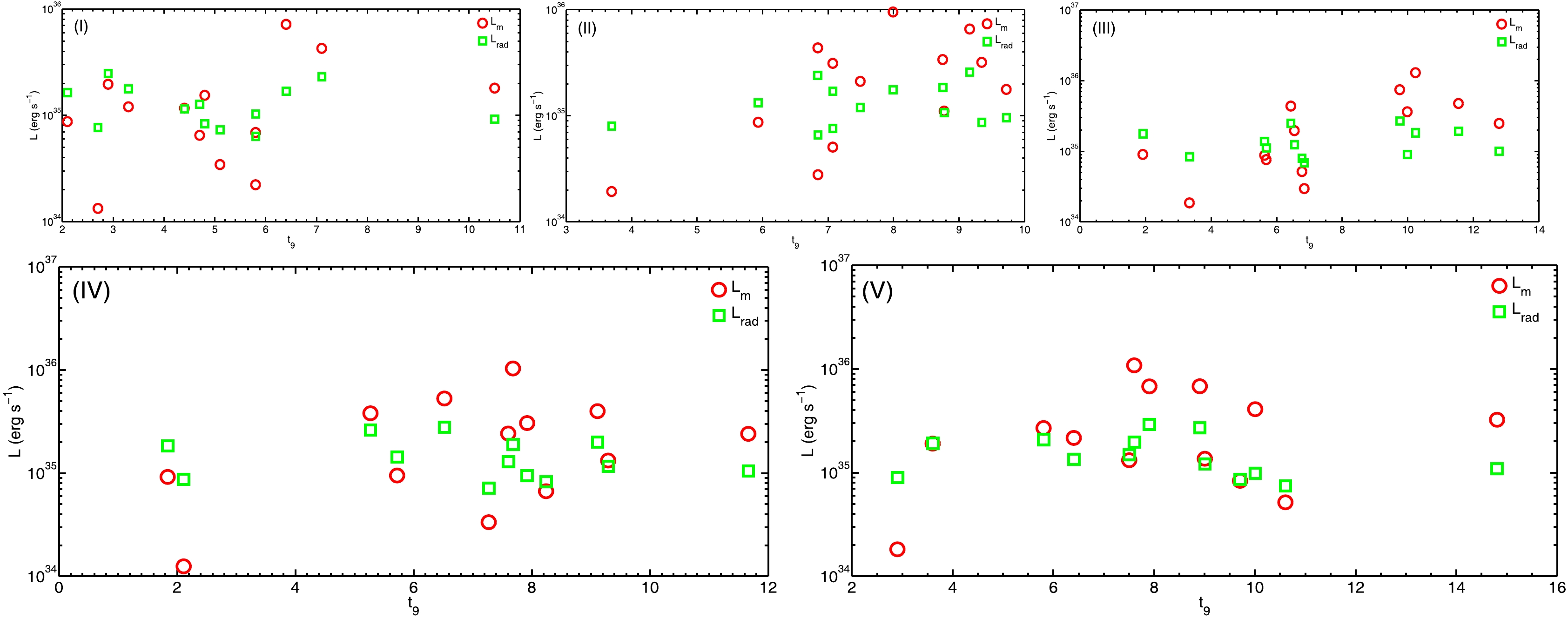
Figure 1. (color online) The luminosities as a function of
$ t_9 $ for the 13 WDs [41] for the five models I$-$ V when$n_{\rm B}=5.99\times10^{31}\rm{cm^{-3}}$ ,$ m=10^{15} $ GeV,$ \sigma_m=10^{-24}\rm{cm^2}, \phi=10^{-26}\rm{cm^{-2}s^{-1}sr^{-1}} $ at the temperature$ T_6=1 $ .
Figure 2. (color online) The luminosities as a function of
$ t_9 $ of the 13 WDs [41] for models I$-$ V when$n_{\rm B}=5.99\times10^{31}\rm{cm^{-3}}$ ,$ m=10^{15} $ GeV,$ \sigma_m=10^{-24}\rm{cm^2}, \phi=10^{-26}\rm{cm^{-2}s^{-1}sr^{-1}} $ at the temperature$ T_6=10 $ .star our results observations $L_{m }$ (I)

$L_{m }$ (II)

$L_{m }$ (III)

$L_{m }$ (IV)

$L_{m }$ (V)

$ L_{\rm{rad}} $ (I)

$ L_{\rm{rad}} $ (II)

$ L_{\rm{rad}} $ (III)

$ L_{\rm{rad}} $ (IV)

$L_{m }$ (V)

1 6.9103e34 1.1107e35 7.6414e34 1.3269e35 1.3639e35 1.0318e35 1.0746e35 1.1187e35 1.1641e35 1.2109e35 2 1.9658e35 6.6000e35 7.4626e35 5.2980e35 6.8110e35 2.4869e35 2.5900e35 2.6962e35 2.8057e35 2.9185e35 3 6.5043e34 8.7231e34 8.7978e34 9.4896e34 1.3202e35 1.2778e35 1.3308e35 1.3854e35 1.4417e35 1.4996e35 4 1.8085e35 1.7795e35 2.4853e35 2.4073e35 3.2420e35 9.2913e34 9.6763e34 1.0073e35 1.0482e35 1.0904e35 5 7.1985e35 9.5522e35 1.2992e36 1.0354e36 1.0871e36 1.6913e35 1.7614e35 1.8336e35 1.9081e35 1.9848e35 6 1.3336e34 1.9390e34 1.8630e34 1.2496e34 1.8224e34 7.7022e34 8.0214e34 8.3505e34 8.6895e34 9.0388e34 7 1.2064e35 3.3998e35 4.7637e35 3.9925e35 2.6970e35 1.7814e35 1.8552e35 1.9313e35 2.0097e35 2.0905e35 8 2.2275e34 2.7936e34 2.9665e34 3.3475e34 5.1790e34 6.3515e34 6.6147e34 6.8861e34 7.1657e34 7.4537e34 9 4.2799e35 4.3831e35 4.3763e35 3.8078e35 6.8228e35 2.3176e35 2.4137e35 2.5127e35 2.6147e35 2.7198e35 10 1.5475e35 3.2020e35 3.6329e35 3.0607e35 4.1003e35 8.3978e34 8.7458e34 9.1046e34 9.4742e34 9.8551e34 11 8.7565e34 3.1336e35 9.0399e34 9.1974e34 1.9093e35 1.6398e35 1.7078e35 1.7779e35 1.8501e35 1.9244e35 12 1.1707e35 2.1183e35 1.9649e35 2.4242e35 2.1660e35 1.1526e35 1.2004e35 1.2496e35 1.3004e35 1.3526e35 13 3.4511e34 5.0855e34 5.1732e34 6.6849e34 8.3500e34 7.3599e34 7.6649e34 7.9794e34 8.3034e34 8.6371e34 Table 7. Comparisons of the calculated luminosities (
$L_{m}$ ) due to the RC effect by MMs with observations ($ L_{\rm{rad}} $ ) for the five models I$-$ V at$n_{\rm B}=5.99\times10^{31}{\rm cm^{-3}}, m=10^{15}$ GeV,$\sigma_m=10^{-24}{\rm cm^2}, \phi=10^{-26}{\rm cm^{-2}s^{-1}sr^{-1}}, T_6=1$ ($ \xi=1.5745\times10^{-15}\rm{cm^{-2}s^{-1}sr^{-1}} $ ).In order to facilitate comparison of our results with the observed data, we define the scale factor
$ k_i $ as the ratio of our results due to the RC effect to the observed luminosity. We note that the largest differences between our results and the observed values are one order of magnitude. For example, based on Table 7 and Table 9 for star 5, the maximal scale factors are$ k_1=4.2562 $ ,$ k_2=5.4231 $ ,$ k_3=7.0851 $ ,$ k_4=5,4264 $ , and$ k_5=5.4772 $ for models I−V, respectively. However, in Table 8 and Table 9, the maximal scale factors for star 5 are$ k_1=13.459 $ ,$ k_2=17.149 $ ,$ k_3=22.405 $ ,$ k_4=17.160 $ and$ k_5=17.321 $ for models I−V, respectively.star Table 7 Table 8 $ k_1 $ 

$ k_2 $ 

$ k_3 $ 

$ k_4 $ 

$ k_5 $ 

$ k_1 $ 

$ k_2 $ 

$ k_3 $ 

$ k_4 $ 

$ k_5 $ 

1 0.66973 1.0336 0.68309 1.1398 1.1264 2.1179 3.2685 2.1601 3.6045 3.5619 2 0.79048 2.5483 2.7678 1.8883 2.3338 2.4997 8.0585 8.7527 5.9714 7.3801 3 0.5090 0.6555 0.6350 0.6582 0.8804 1.6096 2.0728 2.0082 2.0815 2.7840 4 1.9464 1.8390 2.4673 2.2965 2.9733 6.1551 5.8153 7.8022 7.2623 9.4024 5 4.2562 5.4231 7.0851 5.4264 5.4772 13.459 17.149 22.405 17.160 17.321 6 0.1731 0.2417 0.2231 0.1438 0.2016 0.54753 0.7644 0.7055 0.4547 0.6376 7 0.6773 1.8326 2.4666 1.9866 1.2901 2.1416 5.7951 7.8000 6.2821 4.0797 8 0.3507 0.42233 0.4308 0.4672 0.6948 1.1090 1.3355 1.3623 1.4773 2.1972 9 1.8467 1.8159 1.7417 1.4563 2.5085 5.8396 5.7425 5.5076 4.6052 7.9327 10 1.8427 3.6612 3.9902 3.2306 4.1606 5.8273 11.578 12.618 10.216 13.157 11 0.5340 1.8348 0.5085 0.4971 0.9922 1.6886 5.8023 1.6079 1.5721 3.1374 12 1.0157 1.7647 1.5724 1.8642 1.6013 3.2120 5.5806 4.9723 5.8952 5.0638 13 0.4689 0.6635 0.6483 0.8051 0.9668 1.4828 2.0981 2.0502 2.5459 3.0572 star our results observations $L_{m }$ (I)

$L_{m }$ (II)

$L_{m }$ (III)

$L_{m }$ (IV)

$L_{m }$ (V)

$ L_{\rm{rad}} $ (I)

$ L_{\rm{rad}} $ (II)

$ L_{\rm{rad}} $ (III)

$ L_{\rm{rad}} $ (IV)

$L_{m }$ (V)

1 2.1852e35 3.5122e35 2.4164e35 4.1959e35 4.3130e35 1.0318e35 1.0746e35 1.1187e35 1.1641e35 1.2109e35 2 6.2165e35 2.0871e36 2.3599e36 1.6754e36 2.1538e36 2.4869e35 2.5900e35 2.6962e35 2.8057e35 2.9185e35 3 2.0568e35 2.7585e35 2.7821e35 3.0009e35 4.1749e35 1.2778e35 1.3308e35 1.3854e35 1.4417e35 1.4996e35 4 5.7189e35 5.6271e35 7.8593e35 7.6125e35 1.0252e36 9.2913e34 9.6763e34 1.0073e35 1.0482e35 1.0904e35 5 2.2764e36 3.0207e36 4.1083e36 3.2743e36 3.4378e36 1.6913e35 1.7614e35 1.8336e35 1.9081e35 1.9848e35 6 4.2172e34 6.1316e34 5.8913e34 3.9515e34 5.7628e34 7.7022e34 8.0214e34 8.3505e34 8.6895e34 9.0388e34 7 3.8151e35 1.0751e36 1.5064e36 1.2625e36 8.5286e35 1.7814e35 1.8552e35 1.9313e35 2.0097e35 2.0905e35 8 7.0440e34 8.8342e34 9.3808e34 1.0586e35 1.6377e35 6.3515e34 6.6147e34 6.8861e34 7.1657e34 7.4537e34 9 1.3534e36 1.3861e36 1.3839e36 1.2041e36 2.1576e36 2.3176e35 2.4137e35 2.5127e35 2.6147e35 2.7198e35 10 4.8936e35 1.0126e36 1.1488e36 9.6788e35 1.2966e36 8.3978e34 8.7458e34 9.1046e34 9.4742e34 9.8551e34 11 2.7691e35 9.9092e35 2.8587e35 2.9085e35 6.0377e35 1.6398e35 1.7078e35 1.7779e35 1.8501e35 1.9244e35 12 3.7022e35 6.6988e35 6.2135e35 7.6659e35 6.8495e35 1.1526e35 1.2004e35 1.2496e35 1.3004e35 1.3526e35 13 1.0913e35 1.6082e35 1.6359e35 2.1140e35 2.6405e35 7.3599e34 7.6649e34 7.9794e34 8.3034e34 8.6371e34 Table 8. The comparisons of the luminosity (
$L_{m}$ ) due to RC effect by MMs with the observed values ($ L_{\rm{rad}} $ ) for the five models I$-$ V at$n_{\rm B}=5.99\times10^{31}{\rm cm^{-3}}, m=10^{15}$ GeV,$\sigma_m=10^{-24}{\rm cm^2}, \phi=10^{-26}{\rm cm^{-2}s^{-1}sr^{-1}}, T_6=10$ ($ \xi=4.9790\times10^{-15}\rm{cm^{-2}s^{-1}sr^{-1}} $ ).According to the analysis above, our results agree well with observations at lower relativistic densities and temperatures, but the greatest difference is about two orders of magnitude at higher relativistic densities and temperatures in WDs. The good agreement of our calculatedresults with observations shows that our model with the RC effect by MMs yields realistic results, as well as suggesting that the energy source of WDs is the RC effect by MMs.
The monopole flux problem is well known to be a highly challenging and interesting issue. Some scholars have made pioneering work on this subject, such as Freese [32], Parker [39], Kolb & Turner [31], and Freese & Krasteva [40]. In this paper, we discuss this problem by considering the RC effect of MMs. Tables 10 (
$ m=10^{15}\rm{GeV}, \beta=9.4868\times10^{-3} $ ) and 11 ($ m=10^{17}\rm{GeV}, \beta=1.00\times10^{-3} $ ) show the flux of MMs for the four models I$ \sim $ III and V, which correspond to typical asteroseismic correction factor values$ f_{\bigtriangleup\nu}=0.98, 0.99, 1.00, 1.02 $ when$n_{\rm B}=5.99\times10^{31}, 1.89\times10^{32}\rm{cm^{-3}}$ . One can see that the maximum of the monopole flux values are$ 9.0935\times10^{-13}\rm{cm^{-2}s^{-1}sr^{-1}} $ and$ 5.8519\times10^{-13} \rm{cm^{-2}s^{-1}sr^{-1}} $ in Tables 10 and 11, respectively.star $ n_B=5.99\times10^{31}\rm{cm^{-3}} $ 

$ n_B=1.89\times10^{32}\rm{cm^{-3}} $ 

ξ(I) ξ(II) ξ(III) ξ(IV) ξ(V) ξ(I) ξ(II) ξ(III) ξ(IV) ξ(V) 1 2.3509e-13 1.5233e-13 2.3050e-13 1.3813e-13 1.3978e-13 2.3614e-14 1.5301e-14 2.3152e-14 1.3875e-14 1.4041e-14 2 1.9918e-13 6.1786e-14 5.6885e-14 8.3380e-14 6.7465e-14 2.0007e-14 6.2061e-15 5.7139e-15 8.3752e-15 6.7765e-15 3 3.0933e-13 2.4021e-13 2.4794e-13 2.3920e-13 1.7884e-13 3.1070e-14 2.4128e-14 2.4904e-14 2.4026e-14 1.7964e-14 4 8.0892e-14 8.5618e-14 6.3815e-14 6.8559e-14 5.2954e-14 8.1252e-15 8.5999e-15 6.4099e-15 6.8865e-15 5.3190e-15 5 3.6993e-14 2.9033e-14 2.2223e-14 2.9015e-14 2.8746e-14 3.7157e-15 2.9162e-15 2.2322e-15 2.9145e-15 2.8874e-15 6 9.0935e-13 6.5135e-13 7.0573e-13 6.0949e-13 7.8094e-13 9.1340e-14 6.5425e-14 7.0887e-14 7.0998e-14 7.8442e-14 7 2.3248e-13 8.5916e-14 6.3833e-14 7.9257e-14 1.2204e-13 2.3352e-14 8.6299e-15 6.4117e-15 7.9610e-15 1.2259e-14 8 4.4895e-13 3.7281e-13 3.6549e-13 3.3703e-13 2.2661e-13 4.5095e-14 3.7447e-14 3.6711e-14 3.3854e-14 2.2761e-14 9 8.5262e-14 8.6703e-14 9.0402e-14 1.0812e-13 6.2765e-14 8.5642e-15 8.7090e-15 9.0804e-15 1.0860e-14 6.3044e-15 10 8.5442e-14 4.3005e-14 3.9459e-14 4.8737e-14 3.7843e-14 8.5823e-15 4.3196e-15 3.9635e-15 4.8954e-15 3.8011e-15 11 2.9486e-13 8.5810e-14 3.0965e-13 3.1671e-13 1.5870e-13 2.9617e-14 8.6192e-15 3.1103e-14 3.1812e-14 1.5940e-14 12 1.5501e-13 8.9220e-14 1.0013e-13 8.4458e-14 9.8324e-14 1.5570e-14 8.9617e-15 1.0058e-14 8.4834e-15 9.8762e-15 13 3.3578e-13 2.3731e-13 2.4285e-13 1.9557e-13 1.6286e-13 3.3727e-14 2.3837e-14 2.4394e-14 1.9644e-14 1.6359e-14 Table 10. The flux of MMs for the five models I−V (corresponding to typical asteroseismic correction factor values
$ f_{\Delta\nu}= $ 0.98, 0.99, 1.00, 1.01, 1.02) when$m=10^{15}{\rm GeV}, \beta=9.4868\times10^{-3}, n_{\rm B}=5.99\times10^{31}, 1.89\times10^{32}\rm{cm^{-3}}$ .star $n_{\rm B}=5.99\times10^{31}\rm{cm^{-3} }$ 

$n_{\rm B}=1.89\times10^{32}\rm{cm^{-3} }$ 

ξ(I) ξ(II) ξ(III) ξ(IV) ξ(V) ξ(I) ξ(II) ξ(III) ξ(IV) ξ(V) 1 1.5302e-13 9.8450e-14 1.4791e-13 8.8011e-14 8.8428e-14 1.5370e-14 9.8889e-15 1.4857e-14 8.8403e-15 8.8822e-15 2 1.3438e-13 4.1410e-14 3.7874e-14 5.5146e-14 4.4323e-14 1.3498e-14 4.1595e-15 3.8042e-15 5.5391e-15 4.4520e-15 3 1.9655e-13 1.5150e-13 1.5522e-13 1.4864e-13 1.1031e-13 1.9742e-14 1.5218e-14 1.5591e-14 1.4930e-14 1.1080e-14 4 5.5723e-14 5.8607e-14 4.3406e-14 4.6336e-14 3.5561e-14 5.5971e-15 5.8868e-15 4.3599e-15 4.6543e-15 3.5720e-15 5 2.6798e-14 2.0914e-14 1.5918e-14 2.0667e-14 2.0359e-14 2.6918e-15 2.1008e-15 1.5989e-15 2.0759e-15 2.0450e-15 6 4.9950e-13 3.5454e-13 3.8064e-13 5.8519e-13 4.1359e-13 5.0173e-14 3.5612e-14 3.8234e-14 5.8779e-14 4.1543e-14 7 1.5209e-13 5.5812e-14 4.1175e-14 5.0764e-14 7.7618e-14 1.5276e-14 5.6060e-15 4.1359e-15 5.0990e-15 7.7963e-15 8 2.5870e-13 2.1299e-13 2.0702e-13 1.8927e-13 1.2617e-13 2.5985e-14 2.1394e-14 2.0794e-14 1.9011e-14 1.2673e-14 9 6.1421e-14 6.2105e-14 6.4385e-14 7.6561e-14 4.4190e-14 6.1695e-15 6.2382e-15 6.4672e-15 7.6902e-15 4.4387e-15 10 5.8850e-14 2.9433e-14 2.6835e-14 3.2935e-14 2.5410e-14 5.9112e-15 2.9564e-15 2.6955e-15 3.3081e-15 2.5523e-15 11 1.9284e-13 5.5727e-14 1.9968e-13 2.0279e-13 1.0090e-13 1.9370e-14 5.5975e-15 2.0057e-14 2.0370e-14 1.0135e-14 12 9.8741e-14 5.6415e-14 6.2849e-14 5.2620e-14 6.0805e-14 9.9181e-15 5.6666e-15 6.3129e-15 5.2854e-15 6.1076e-15 13 1.9890e-13 1.3942e-13 1.4150e-13 1.1301e-13 9.3331e-14 1.9979e-14 1.4004e-14 1.4213e-14 1.1351e-14 9.3746e-15 Table 11. The flux of MMs for the five models I−V (corresponding to typical asteroseismic correction factor values
$ f_{\Delta\nu}= $ 0.98, 0.99, 1.00, 1.01, 1.02) when$m=10^{17}{\rm GeV}, \beta=1.0\times10^{-3}, n_{\rm B}=5.99\times10^{31}, 1.89\times10^{32}\rm{cm^{-3}}$ .It is very interesting to note that the monopole flux decreases as
$n_{\rm B}$ increases from$ 5.99\times10^{31} $ to$ 1.89\times 10^{32}\rm{cm^{-3}} $ in Tables 10 and 11. This is not hard to understand according to Eq. (10). Based on our calculations above from Tables 10, due to the RC effect by MMs, we obtain new limits on the MM flux of$\xi\leq 9.0935\times 10^{-13}\rm{cm^{-2}s^{-1}sr^{-1}}$ and$\xi\leq 9.1340\times 10^{-14} \rm{cm^{-2}s^{-1}sr^{-1}}$ when$n_{\rm B}=5.99\times10^{31} \rm{cm^{-3}}$ and$ 1.899\times 10^{32}\rm{cm^{-3}} $ , respectively. In Table 11, the new limits on the MM flux are$\xi\leq 4.9950 \times10^{-13}\rm{cm^{-2}s^{-1}sr^{-1}}$ and$\xi\leq 5.0173\times10^{-14} \rm{cm^{-2}s^{-1}sr^{-1}}$ when$n_B=5.99\times10^{31}$ and$ 1.899\times10^{32} $ , respectively.Based on the above analysis, we obtain new limits on the MM flux of
$\xi\leq 9.0935\times10^{-13} \rm{cm^{-2}s^{-1}sr^{-1}}$ , and$ \xi\leq 4.9950\times10^{-13}\rm{cm^{-2}s^{-1}sr^{-1}} $ at$n_{\rm B}=5.99\times10^{31}\rm{cm^{-3}}$ when$ m=10^{15}\rm{GeV}, \beta=9.4868\times10^{-3} $ , and$ m=10^{17}\rm{GeV}, \beta=10^{-3} $ , respectively. When we estimate the number of MMs captured, the MM luminosity and the limit of the MM flux, as samples, we consider the 13 RGB stars in our MM model for the following reasons. First, WDs originate from RGB stars. Second, compared with WDs, RGB stars have a very large surface area. According to Eq. (10), we expect RGB phases to capture more MMs during their evolution period. Third, since the MM is a superheavy particle, when MMs are captured by an RGB, they will be deposited in the star core. If all MMs captured by RGBs remain, their number will be much larger than that of those captured by WDs. Thus, the number of MMs calculated inside an WD will be more accurate than for MMs captured only during the WD phase. For example, Freese et al. [51] showed that if the MMs captured by stars in the main sequence stage all survive, the MM flow due to neutron star catalysis can be strengthened by up to 7 orders of magnitude. Finally, based on Schwarzschid [52], the nuclear energy generation rates of the proton-proton and CNO cycle are$ \epsilon_{\rm{pp}}\approx10\rho_{100}T_7^4 \rm{erg\; g^{-1}s^{-1}} $ and$ \epsilon_{\rm{CNO}}\approx8\rho_{100}T_7^{16} \rm{erg\; g^{-1}s^{-1}} $ , respectively (where$ T_7=T/10^7\rm{K} $ is the temperature, and$ \rho_{100}=\rho/100 $ is the density). Based on the discussions fof Bjork et al. [53], we may select the mass of the outer layer of the RGB as being from$0.005\sim0.02 {M}_{\odot}$ (the main component is hydrogen). Thus, when$T_7=0.1-1$ ,$ \rho_{100}\sim10^{-4} $ , and we obtain a proton-proton nuclear energy generation rate of$10^{24} - 10^{28} \rm{ergs\; s^{-1}}$ , which is$\ll L_m=10^{34} - 10^{36}\rm{ergs\; s^{-1}}$ in our calculations. Based on the above analysis, and the fact that RGB stars are the origins of WDs, we therefore have$ L_{\rm{m}}\approx L_{\rm{rad}} $ .One can also conclude that with the increasing number of MMs captured, the luminosity due to the RC effect by MMs increases linearly with time until it becomes the main contribution to the total luminosity. One can even observe that for some of the oldest white dwarfs, the luminosity may have passed its minimum and some reheating may have occurred.
It may be suggested that the annihilation of magnetic and antimagnetic monopoles could result in a significant reduction in the number of monopoles and the catalytic luminosity of the monopoles in the WDs. Dicus et al. [54] calculated the annihilation cross sections of magnetic monopoles and antimonopoles caused by two-body and three-body recombination. Their results show that this kind of annihilation has little effect on the flux and luminosity of the monopole. On the other hand, some WDs may have magnetic fields of up to
$ 10^5 $ G according to observations. The forces generated by the magnetic field inside the white dwarf must balance the gravitational and Coulomb interactions.The magnetic field may keep the monopole and antimonopole distributions far enough apart for annihilation to be negligible.On the other hand, neutrino emission in WDs is a very interesting issue. Based on the discussions of Althaus et al. [55], when WD is very hot, neutrino emissions could be a major source of cooling. However, based on the relatively low temperature environment of WDs (e.g.,
$ T_6=1, 10 $ in our paper) we discussed the heating resource problem with our MMs model. The neutrino processes inside WDs at such low temperatures (e.g.,$ T_6=1 $ ) may not be the main cooling process (see discussions by Itoh et al. [56]). On the other hand, Izawa [57] also discussed the neutrinos emitted according to Eqs. (23), (24) in his paper and calculated the neutrino emitted per one nucleon decay at low and high energy components, finding that these neutrino losses did not affect the structure or evolution of Rubakov stars because the energy lost through the neutrino emission is smaller than 100 MeV per one nucleon decayn although about two neutrinos are emitted furing the decay of one nucleon.According to the above analysis, one can see that MMs pass through space to be captured by WDs. MMs trapped inside a WD can catalyze the decay of nuclei, which can function as an energy source to keep the WDs hot.
-
We have presented five MMs models of WD energy resources to discuss their cooling based on certain observations of 13 RGB stars. We find that the number of MMs captured can reach a maximum value of
$ 9.1223\times10^{24} $ when$m=10^{17}\;\;{\rm GeV}, \; n_{\rm B}=5.99\times10^{31}\; \rm{cm^{-3}}, \phi=7.59\times10^{-26}\;\;\rm{cm^{-2}s^{-1}sr^{-1}}$ . The good agreement with observations of our luminosities due to the RC effect by MMs calculated for WDs shows that our model is reasonable. We conclude that the energy source of WDs may be the RC effect. Due to the RC effect by MMs, we obtain a new limit of MM flux of$\xi\leq 9.0935\times 10^{-13} \;\; \rm{cm^{-2}s^{-1}sr^{-1}}$ and$\xi\leq 4.9950\times10^{-13}\;\;\rm{cm^{-2}s^{-1}sr^{-1}}$ at$n_{\rm B}=5.99\times 10^{31} \rm{cm^{-3}}$ when$m=10^{15}\rm{GeV}, \;\beta=9.4868\times10^{-3}$ , and$m=10^{17}\rm{GeV}, \;\beta=10^{-3}$ , respectively.In this paper, the main highlights may be given as follows. First, we created detailed estimates of the cooling ages of 13 RGB stars using the packages BASTA [42], isochrones [43], isoclassify [44], PARAM [45,46], and scaling-giants [47]. Second, we proposes five new models to discuss the energy resources and the cooling of WDs and compare the luminosities with observations for 13 RGB stars due to the RC effect. Finally, the new limit of the MM flux is obtained based on our models.
As is widely known, research on MMs haa always been a hot frontier topic in the fields of nuclear physics and astrophysics. The search for MMs remians a difficult and challenging problem, and the flux of magnetic monopoles in the universe remains uncertain. The neutrino emissivity rates due to the RC effect also may play a key role in the process of WD and neutron star evolution. These challenging problem will be our future issues.
New insights into the limit of the magnetic monopole flux and the heating source in white dwarfs
- Received Date: 2023-04-09
- Available Online: 2023-08-15
Abstract: Based on the magnetic monopole (MM) catalytic nuclear decay (Rubakov-Callan (RC) effect), we propose five new models to discuss the limit of the MM flux and the heating energy resources of white dwarfs (WDs) based on observations of 13 red giant branch (RGB) stars. We find that the number of MMs captured can reach a maximum value of


 DownLoad: