


 Abstract
 HTML
HTML Reference
 Related
 PDF
PDF


-
Decay parameters are the key for connecting theoretical models with experimental studies. Two-body decays can provide a clean environment to examine the properties of baryons, including polarization and decay parameters. This type of an environment can thus enable the verification of theoretical models such as perturbative QCD [1]. CP violation (CPV) is observed in
$K^0,\; B^0 ,$ and$ D^0 $ meson decays [2−5], and the experimental results are consistent with the Standard Model predictions. In the baryonic decay, the magnitude of CPV is predicted only in the range of$10 ^ { -4 } - 10 ^ { -5 }$ with standard model (SM) [6, 7]. However, the magnitude can be$ 10 ^{ -3} $ in certain new physics models such as those presented in Refs. [8−13]. However, it is still not sufficiently large to understand the asymmetry of the matter and anti-matter in the universe. Therefore, it is important to expand the sources of CPV, especially in the baryonic sector.BESIII at BEPCII has accumulated approximately 10 billion
$ J/\psi $ mesons, and a large statistic of hyperon-antihyperon pairs produced from$ J/\psi $ decays. Specifically,$ {e^+e^-} $ collision experiment has a natural advantage over$ pp $ collision or fix-targed experiments in measuring high accuracy due to its lower background. An important study related to our analysis has been conducted and published in Nature [14] with a significantly higher accuracy improvement in measurement. Exploring evidence of CPV within BESIII experiments continues to hold promise, warranting further and deeper analysis of the data at hand.Particle Data Group (PDG) provides an evaluation of
$\alpha_{\Xi^0 \to \Lambda \pi^0}=-0.349 \pm 0.009$ via dividing$\alpha({\Xi^0})\alpha_{-}({\Lambda})$ by a current average$\alpha_{-}({\Lambda})$ according to the measurements obtained in recent years [15]. Furthermore,$\alpha_{\Xi^0\to \Lambda \gamma}$ is equal to$-0.704 \pm0.019_{\rm stat} \pm 0.064_{\rm syst}$ based on the latest result meausred by NA481 Collaboration, utilizing a data sample of 52,000 events [16]. Based on the data, a statistical uncertainity of$ 2.70 $ % can be realized in the radiative decay$\Xi^0\to \Lambda \gamma$ . As more data become available and simultaneous measurements are made on its conjugate decay channel, we can obtain more precise asymmetric parameters. This serves as a probe to search for evidence of CPV in these decays, enhancing our understanding of the CPV mechanism in baryons.In this study, in Sec. II, we formulate the observables of parity violation and CPV as proposed in Ref. [17]. Diverging from the traditional definition proposed by T. D. Lee and C. N. Yang [18], which uses partial wave amplitudes, we employ the helicity formalism to present these asymmetric parameters. This method provides convenience for experimental physicists when estimating or predicting these properties. We formulate the joint spin density matrix (SDM) of baryon pairs
$ \Xi^0{\bar{\Xi}}^0 $ and$ \Lambda {\bar{\Lambda}} $ in Sec. IV. A sensitivity estimation on the asymmetric parameters of parity violation is performed in Sec. V. This serves as a reference for precise measurements of these decay channels in future experiments with high statistical significance. -
In the two-body decays with parity conservation, the helicity amplitudes satisfy the following symmetry.
$ \begin{array}{*{20}{l}} A^J_{\text{λ}_1,\text{λ}_2}=\eta\eta_1\eta_2(-1)^{J-s_1-s_2} A^J_{-\text{λ}_1, -\text{λ}_2}, \end{array} $

(1) where
$ J, s_1 ,$ and$ s_2 $ denote the spins of the mother particle and two daughter particles, respectively.$ \text{λ},~ \text{λ}_1, $ and$ \text{λ}_2 $ denote their helicity values, and$\eta, ~\eta_1,$ and$ \eta_2 $ denote their intrinsic parity values, respectively. Assuming that the decays listed in Table 1 are parity conserved, the corresponding helicity amplitudes,$ A,\; B,\; F,\; G, $ and H, satisfy the following.decay helicity angle helicity amplitude $ J/\psi\to\Xi^0({\text{λ}}_1){\bar{\Xi}}^0({\text{λ}}_2) $ 

( $ \theta_0,\phi_0 $ )

$ A_{{\text{λ}}_1,{\text{λ}}_2} $ 

$\Xi^0({\text{λ} }_1^{\prime})\to{\Lambda }({\text{λ} }_3)\pi^0$ 

( $ \theta_1,\phi_1 $ )

$ B_{{\text{λ}}_3} $ 

${\bar{\Xi} }^0({\text{λ} }_2^{\prime})\to{\bar{ {\Lambda } } }({\text{λ} }_4)\gamma({\text{λ} }_5)$ 

( $ \theta_2,\phi_2 $ )

$ F_{{\text{λ}}_5,{\text{λ}}_4} $ 

${\Lambda }({\text{λ} }'_3)\to p({\text{λ} }_6)\pi^-$ 

( $ \theta_3,\phi_3 $ )

$ H_{{\text{λ}}_6} $ 

${\bar{ {\Lambda } } }({\text{λ} }'_4)\to {\bar{p} }({\text{λ} }_7) \pi^+$ 

( $ \theta_4,\phi_4 $ )

$ G_{{\text{λ}}_7} $ 

Table 1. Definition of helicity angles and amplitudes in each decay, where
$\text{λ}_i$ denotes the helicity values for the corresponding particles.$ \begin{aligned}[b] A_{-\frac{1}{2},-\frac{1}{2}}=&A_{\frac{1}{2}, \frac{1}{2}}, A_{-\frac{1}{2},\frac{1}{2}}=A_{\frac{1}{2}, -\frac{1}{2}},\\ B_{\frac{1}{2}}=&-B_{-\frac{1}{2}}, F_{1, \frac{1}{2}}=F_{-1, -\frac{1}{2}},\\ H_{\frac{1}{2}}=&-H_{-\frac{1}{2}}, G_{\frac{1}{2}}=-G_{-\frac{1}{2}}, \end{aligned} $

(2) where amplitude F can be expressed as
$ F_{\text{λ}_5,\text{λ}_4} $ as opposed to$ F_{\text{λ}_4,\text{λ}_5} $ to maintain consistency with its definition in Ref. [16]. However, the parity violation in weak decay renders the aforementioned equations invalid. Therefore, we define four asymmetric parameters to describe the parity violation as follows:$ \begin{aligned}[b] \alpha_{\Xi^0\to \Lambda \pi^0}=&\dfrac{|B_{\frac{1}{2}}|^2-|B_{-\frac{1}{2}}|^2}{|B_{\frac{1}{2}}|^2+|B_{-\frac{1}{2}}|^2},\\ \alpha_{{\bar{\Xi}}^0\to {\bar{\Lambda}} \gamma}=&\dfrac{|F_{-1,-\frac{1}{2}}|^2-|F_{1,\frac{1}{2}}|^2}{|F_{-1,-\frac{1}{2}}|^2+|F_{1,\frac{1}{2}}|^2},\\ \alpha_{\Lambda\to p \pi^-}=&\dfrac{|H_{\frac{1}{2}}|^2-|H_{-\frac{1}{2}}|^2}{|H_{\frac{1}{2}}|^2+|H_{-\frac{1}{2}}|^2},\\ \alpha_{{\bar{\Lambda}}\to {\bar{p}} \pi^+}=&\dfrac{|G_{\frac{1}{2}}|^2-|G_{-\frac{1}{2}}|^2}{|G_{\frac{1}{2}}|^2+|G_{-\frac{1}{2}}|^2}. \end{aligned} $

(3) The four parameters defined in this study are numerically equivalent to the partial-wave amplitudes and are consistent with the parameter values provided in the PDG convention.
Furthermore, if CP conservation holds in charge conjugate decays, then the parameters of the conjugate decays have the same absolute values but bear the opposite sign when compared to the aforementioned four parameters, i.e.,
$\alpha_{{\bar{\Xi}}^0\to {\bar{\Lambda}} \pi^0}= -\alpha_{\Xi^0\to \Lambda \pi^0}$ ,$ \alpha_{\Xi^0\to \Lambda \gamma}=-\alpha_{{\bar{\Xi}}^0\to {\bar{\Lambda}} \gamma} $ ,$ \alpha_{\Lambda\to p \pi^-}= -\alpha_{{\bar{\Lambda}}\to {\bar{p}} \pi^+} $ . Thus, we can define three observables characterizing the degree of CPV as follows:$ \begin{aligned}[b] & A_{CP}^{1}=\dfrac{\alpha_{{\bar{\Xi}}^0\to {\bar{\Lambda}} \pi^0}+\alpha_{\Xi^0\to \Lambda \pi^0}}{\alpha_{{\bar{\Xi}}^0\to {\bar{\Lambda}} \pi^0}-\alpha_{\Xi^0\to \Lambda \pi^0}},\\& A_{CP}^{2}=\dfrac{\alpha_{\Xi^0\to \Lambda \gamma}+\alpha_{{\bar{\Xi}}^0\to {\bar{\Lambda}} \gamma}}{\alpha_{\Xi^0\to \Lambda \gamma}-\alpha_{{\bar{\Xi}}^0\to {\bar{\Lambda}} \gamma}},\\ & A_{CP}^{3}=\dfrac{\alpha_{\Lambda\to p \pi^-}+\alpha_{{\bar{\Lambda}}\to {\bar{p}} \pi^+}}{\alpha_{\Lambda\to p \pi^-}-\alpha_{{\bar{\Lambda}}\to {\bar{p}} \pi^+}}. \end{aligned} $

(4) The non-zero value of the asymmetric parameters in Eqs. (3) and (4) indicates that there is CPV in the decay. Experimentally, by measuring these conjugate decays separately, we can obtain the corresponding CP violated information. We can shorten
$\alpha_{\Xi^0\to \Lambda \pi^0},\; \alpha_{{\bar{\Xi}}^0\to {\bar{\Lambda}} \gamma},\; \alpha_{\Lambda\to p \pi^-} $ ,$\alpha_{{\bar{\Lambda}}\to {\bar{p}} \pi^+}$ as$\alpha_{\Xi^0},\; \alpha_{{\bar{\Xi}}^0},\; \alpha_{\Lambda},\; \alpha_{{\bar{\Lambda}}}$ in the following narrative.When describing parity violation, the helicity amplitudes are more straightforward when compared to the covariant amplitude. The helicity formalism is widely used in experimental measurements [19−23]. Helicity amplitudes are also used to form the SDM of particles in a decay, and the SDM contains all the dynamical information of the decay. The angular distributions and polarization are also easily derived from SDM. Experimentally, the values of these parameters can be determined by fitting the joint angular distribution to the data [24]. The helicity amplitude can be expanded into the L-S coupling of the partial wave amplitude through the Clebsch– Gordan coefficient. In view of the convenience of using the helicity amplitude, we use it to analyze the cascade decay.
-
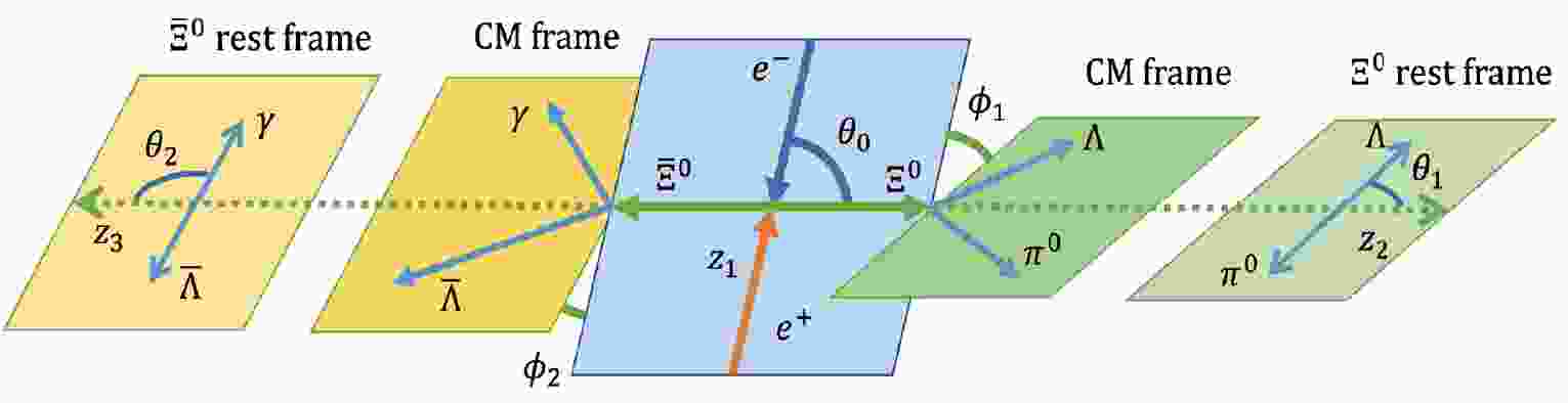
In this analysis, we use the helicity reference frame to describe the full decay chain. The properties of helicity amplitude can be found in Ref. [25]. The helicity angles of the various levels of decay are shown in Fig. 1, Fig. 2, and Fig. 3. The corresponding amplitudes are listed in Table 1.
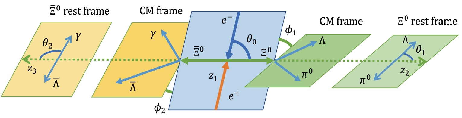
Figure 1. (color online) Definition of helicity angles in
$J/\psi\to $ $ \Xi^0 (\Lambda \pi^0) {\bar{\Xi}}^0({\bar{\Lambda}} \gamma)$ decays.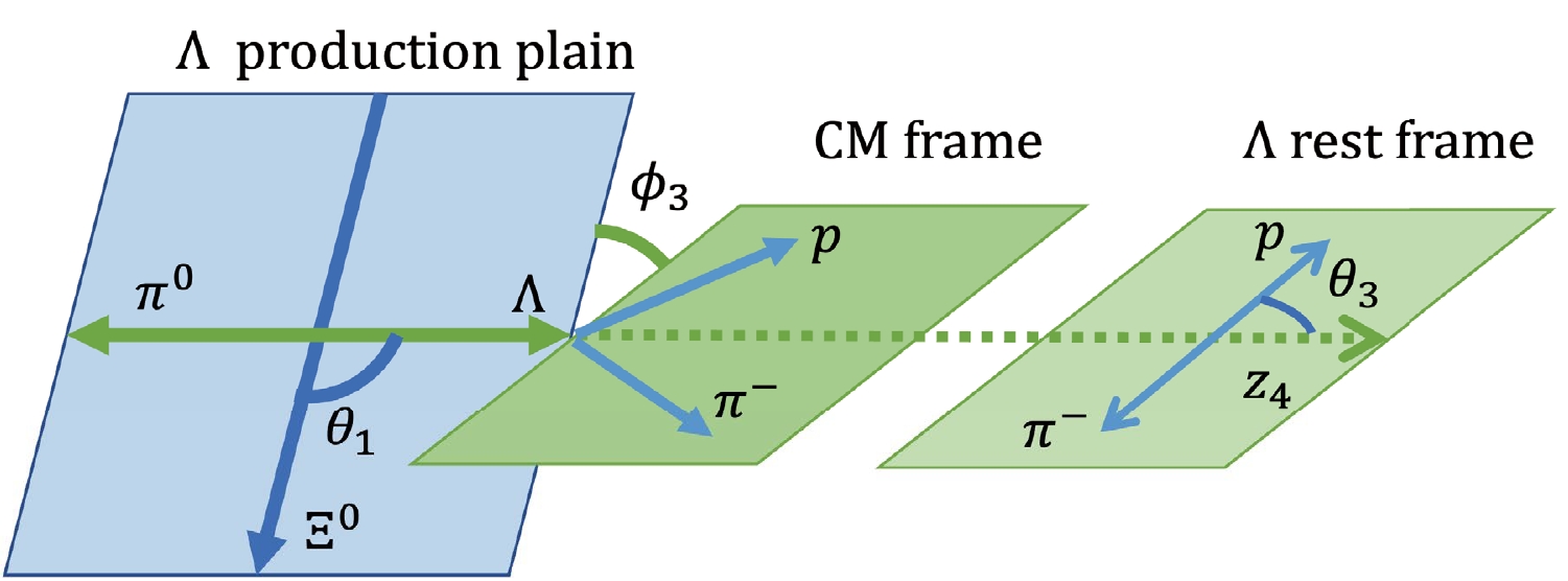
Figure 2. (color online) Definition of helicity angles in
$ \Lambda \to p \pi^0 $ decay.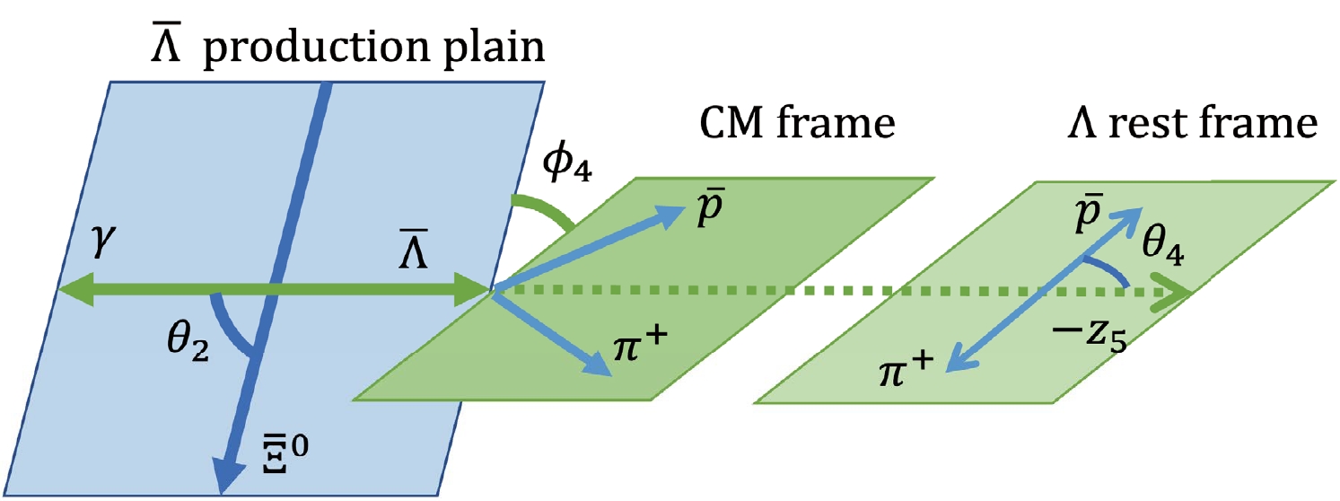
Figure 3. (color online) Definition of helicity angles in
$ {\bar{\Lambda}} \to {\bar{p}} \pi^+ $ decay.In this section, we specify that the momentum p with superscript L represents the momentum in the laboratory system, and the momentum without the superscript represents the momentum after the boost operation to the rest frame of its mother particle. In experiments, the momenta
$ \vec{p}^{L}_{{\Lambda}} $ by$ \vec{p}^{L}_p $ and$ \vec{p}^{L}_{\pi^-} $ are reconstructed from the detection information. Then, we boost$ \vec{p}^{L}_p $ and$ \vec{p}^{L}_{\pi^-} $ to Λ rest frame, and$ \theta_3 $ describes the angle between$ \vec{p}_p $ (in the Λ rest frame) and$ z_4 $ axis. The angle between Λ production plane and its decay plane is defined as$ \phi_3 $ . As for other helicity angles$ (\theta_i, \phi_i), (i=0,1,2,4) $ , they can be calculated by the same operation as illustration Fig. 1 and Fig. 2. It should be noted that$ z_5 $ axis along the opposite direction of$ \vec{p}_{{\bar{\Lambda}}} $ and$ \theta_2 $ describe the angle between$ \vec{p}_{\gamma} $ (in the$ {\bar{\Xi}}^0 $ rest frame) and$ z_3 $ axis. Here, we list all the helicity angle expressions,$ \begin{split} \theta_0 =& \arccos\left({\dfrac{\vec{p}_{{\Xi^0}} \cdot \vec{p}_{{e^+}}}{|\vec{p}_{{\Xi^0}}| \cdot |\vec{p}_{{e^+}}|}}\right),\; \; \; \; \; \; \; \phi_0 = 0,\\ \theta_1 =& \arccos\left({\dfrac{\vec{p}_{{\Xi^0}} \cdot \vec{p}_{{\Lambda}}}{|\vec{p}_{{\Xi^0}}| \cdot |\vec{p}_{{\Lambda}}|}}\right), \phi_1 =\arccos({ |\vec{n}_{J/\psi} \cdot \vec{n}_{\Xi^0}|}),\\ \theta_2 =& \arccos\left({\dfrac{\vec{p}_{{\bar{\Xi}}^0} \cdot \vec{p}_{\gamma}}{|\vec{p}_{{\bar{\Xi}}^0}| \cdot |\vec{p}_{\gamma}|}}\right), \phi_2 = \arccos({ |\vec{n}_{J/\psi} \cdot \vec{n}_{{\bar{\Xi}}^0}|}),\\ \theta_3 =&\arccos\left({ \dfrac{\vec{p}_{{\Lambda}} \cdot \vec{p}_{{p}}}{|\vec{p}_{{\Lambda}}| \cdot |\vec{p}_{{p}}|}}\right), \phi_3 = \arccos({|\vec{n}_{\Xi^0} \cdot \vec{n}_{\Lambda}|}),\\ \theta_4 =& \arccos\left({\dfrac{\vec{p}_{{\bar{\Lambda}}} \cdot \vec{p}_{{\bar{p}}}}{|\vec{p}_{{\bar{\Lambda}}}| \cdot |\vec{p}_{{\bar{p}}}|}}\right), \phi_4 = \arccos({|\vec{n}_{{\bar{\Xi}}^0} \cdot \vec{n}_{{\bar{\Lambda}}}|}), \end{split} $

(5) where unit vectors
$ \vec{n}_{m} $ in the rest frame of m decay plane are defined with the momenta of those particles as follows:$ \begin{aligned}[b] \vec{n}_{J/\psi} =& \dfrac{\vec{p}_{e^+}\times{\vec{p}_{\Xi^0}}}{|\vec{p}_{e^+}| \cdot |\vec{p}_{\Xi^0}| \cdot \sin\theta_0}, \quad \vec{n}_{\Xi^0} = \dfrac{\vec{p}_{\Xi^0}\times{\vec{p}_{\Lambda}}}{|\vec{p}_{\Xi^0}| \cdot |\vec{p}_{\Lambda}| \cdot \sin\theta_1},\\ \vec{n}_{{\bar{\Xi^0}}} =& \dfrac{\vec{p}_{{\bar{\Xi}}^0}\times{\vec{p}_{\gamma}}}{|\vec{p}_{{\bar{\Xi}}^0}| \cdot |\vec{p}_{\gamma}| \cdot \sin\theta_2}, \quad \vec{n}_{\Lambda} = \dfrac{\vec{p}_{\Lambda}\times{\vec{p}_{p}}}{|\vec{p}_{\Lambda}| \cdot |\vec{p}_{p}| \cdot \sin\theta_3},\\ \vec{n}_{{\bar{\Lambda}}} =& \dfrac{\vec{p}_{{\bar{\Lambda}}}\times{\vec{p}_{{\bar{p}}}}}{|\vec{p}_{{\bar{\Lambda}}}| \cdot |\vec{p}_{{\bar{p}}}| \cdot \sin\theta_4}. \end{aligned} $

(6) -
Given that the SDM contains all the dynamical information in the decay, we first calculate the SDM of baryons in each step of decay, and then derive the angular distributions and expression to present baryon polarization [25, 26].
-
For a spin of
$ -\dfrac{1}{2} $ for a particle like$ \Xi^0 $ , the SDM can be expressed as follows:$ \begin{array}{*{20}{l}} \rho^{\Xi^0}= \left( \begin{array}{cc} \rho^{\Xi^0}_{\frac{1}{2}, \frac{1}{2}} & \rho^{\Xi^0}_{\frac{1}{2}, -\frac{1}{2}} \\ \rho^{\Xi^0}_{-\frac{1}{2}, \frac{1}{2}} & \rho^{\Xi^0}_{-\frac{1}{2}, -\frac{1}{2}} \end{array} \right). \end{array} $

(7) The joint SDM of
$ \Xi^0 {\bar{\Xi}}^0 $ can be constructed in the form of$ \rho^{\Xi^0} \otimes \rho^{{\bar{\Xi}}^0} $ , and its elements can be directly calculated as follows:$ \begin{aligned}[b] \rho^{\Xi^0{\bar{\Xi}}^0}_{\text{λ}_1,\text{λ}_2,\text{λ}_1',\text{λ}_2'}\propto&\displaystyle\sum_{\text{λ},\text{λ}'}\rho_{\text{λ},\text{λ}'}^{\psi}D^{J*}_{\text{λ},\text{λ}_1-\text{λ}_2}(\phi_0,\theta_0,0)\\ \times& D^{J}_{\text{λ}',\text{λ}_1'-\text{λ}_2'}(\phi_0,\theta_0,0)A_{\text{λ}_1,\text{λ}_2}A^*_{\text{λ}'_1,\text{λ}'_2}, \end{aligned} $

(8) where the SDM of
$ J/\psi $ produced from$ e^+e^- $ annihilation can be described as$ \rho_{\text{λ},\text{λ}'}^{\psi}=\dfrac{1}{2}\mathrm{diag}\{1,0,1\} $ [27], and$ D^{J}_{\text{λ}_i,\text{λ}_k} (\phi_0,\theta_0,0) $ is the Wigner-D function. Given that the decay of$ J/\psi $ into$ \Xi^0{\bar{\Xi}}^0 $ via strong interactions conserves the parity, the helicity amplitudes satisfy the equations listed in Eq. (2) i.e.,$ A_{-\frac{1}{2},-\frac{1}{2}}=A_{\frac{1}{2}, \frac{1}{2}}, A_{-\frac{1}{2},\frac{1}{2}}=A_{\frac{1}{2}, -\frac{1}{2}} $ . The angular distribution of$ J/\psi \to \Xi^0 {\bar{\Xi}}^0 $ can be expressed as follows:$ \begin{aligned}[b] I(\theta_0) \propto\;\;& \mathrm{Tr}\left[\rho^{\Xi^0{\bar{\Xi}}^0}\right]=\left|A_{\frac{1}{2},\frac{1}{2}}\right|^2 \sin ^2\theta _0 \\ & +\frac{1}{4} \left|A_{\frac{1}{2},-\frac{1}{2}}\right|^2 \left(\cos 2 \theta _0+3\right). \end{aligned} $

(9) If we select
$ \begin{array}{*{20}{l}} \alpha_\psi=\dfrac{{\left|A_{\frac{1}{2},-\frac{1}{2}}\right|^2-2\left|A_{\frac{1}{2},\frac{1}{2}}\right|^2}}{{\left|A_{\frac{1}{2},-\frac{1}{2}}\right|^2+2\left|A_{\frac{1}{2},\frac{1}{2}}\right|^2}}, \end{array} $

(10) then the angular distribution can be reduced to the formula commonly used in experiments as follows:
$ \begin{array}{*{20}{l}} I(\theta_0) \propto 1+\alpha _\psi\cos ^2\theta _0, \end{array} $

(11) where
$ \alpha_{\psi } $ denotes the angular distribution parameter.On the other hand, the joint SDM of
$ \Xi^0 {\bar{\Xi}}^0 $ can also be expressed by the real multipole parameters$ Q^{1}_{i,j} $ as follows:$ \begin{array}{*{20}{l}} \rho^{\Xi^0{\bar{\Xi}}^0}=\dfrac{Q^{1}_{0,0}}{4}\bigg[I+\displaystyle\sum_{\overline{i,j=0}}^{3}Q^{1}_{i,j}\sigma^{\Xi^0}_i\otimes\sigma^{{\bar{\Xi}}^0}_j\bigg], \end{array} $

(12) where the superscript of
$ Q^{1}_{i,j} $ is used to distinguish from parameters$ Q^{2}_{i,j} $ used in Eq. (23),$ {I} $ is a$ 4 \times 4 $ identity matrix, and σ is Pauli matrix [27]. Here,$ \sigma_i $ or$ \sigma_j\; (i,j = 1, 2, 3) $ correspond to$ \sigma_x, \sigma_y, \sigma_z $ , and i or$ j = 0 $ denotes a$ 2\times 2 $ identity matrix. Specifically,$ \overline{i,j=0} $ implies that they cannot be 0 at the same time.$ Q^1_{i, j} $ can be calculated by$Q^{1}_{0,0}= \mathrm{Tr} \rho^{\Xi^0{\bar{\Xi}}^0}, Q^{1}_{0,0}Q^{1}_{i,j}=\mathrm{Tr}\left[\sigma_i\otimes\sigma_j\cdot \rho^{\Xi^0{\bar{\Xi}}^0}\right]$ . In this manner, multipole parameters$ Q^1_{i, j} $ can be expressed with the helicity amplitudes as listed in Eq. (A2).For the decay
$ J/\psi \to \Xi^0 {\bar{\Xi}}^0 $ ,$ Q^1_{0, 0} $ denotes the unpolarized decay rate. The degree of$ \Xi^0 $ linear polarization can be expressed as$ \mathcal{P}_x^{\Xi^0}=Q^{1}_{1,0},\mathcal{P}_y^{\Xi^0}=Q^{1}_{2,0} $ and longitudinal polarization$ \mathcal{P}_z^{\Xi^0}=Q^{1}_{3,0} $ . For the$ {\bar{\Xi}}^0 $ , they are$ \mathcal{P}_x^{{\bar{\Xi}}^0}= Q^{1}_{0,1},\mathcal{P}_y^{{\bar{\Xi}}^0}=Q^{1}_{0,2} $ , and$ \mathcal{P}_z^{{\bar{\Xi}}^0}=Q^{1}_{0,3} $ . Given that the parity is conserved in the$ J/\psi $ decay, the polarization expressions is as follows:$ \begin{aligned}[b] \mathcal{P}^{\Xi^0}_x =& -\mathcal{P}^{{\bar{\Xi}}^0}_x=0,\; \; \; \; \; \; \mathcal{P}^{\Xi^0}_z = -\mathcal{P}^{{\bar{\Xi}}^0}_z=0,\\ \mathcal{P}^{\Xi^0}_y =& -\mathcal{P}^{{\bar{\Xi}}^0}_y = \dfrac{\sqrt{1-\alpha_{\psi}^2} \sin{2\theta_0} \sin{\Delta_a}}{2(1+\alpha_{\psi} \cos^2{\theta_0})}, \end{aligned} $

(13) where
$ \Delta _a = \xi_{\frac{1}{2},-\frac{1}{2}}-\xi_{\frac{1}{2},\frac{1}{2}} $ denotes the phase difference of the two amplitudes$ A_{{1\over2},-{1\over2}},A_{{1\over2},{1\over2}} $ . Obviously, whether the transverse polarization exists or not depends on the phase angle difference$ \Delta _a $ . -
In these two decays
$ \Xi^0 \to \Lambda \pi^0 $ and$ {\bar{\Xi}}^0 \to {\bar{\Lambda}} \gamma $ , the parity violation can be revealed by the study of the angular distribution of the decaying particle or by the measurement of the polarization. The joint angular distribution$ I(\theta_0,\theta_1,\phi_1,\theta_2,\phi_2) $ of this decay can be calculated by the joint SDM of$ \Xi^0 {\bar{\Xi}}^0 $ as follows:$ \begin{aligned}[b] I(\theta_0, \theta_1, \phi_1, \theta_2, \phi_2) \propto&\displaystyle\sum_{\text{λ}_i,\text{λ}'_i}\rho^{\Xi^0{\bar{\Xi}}^0}_{\text{λ}_1,\text{λ}_2;\text{λ}'_1,\text{λ}'_2} D^{\frac{1}{2}*}_{\text{λ}_1,\text{λ}_3}(\theta_1,\phi_1)\\ \times&D^{\frac{1}{2}}_{\text{λ}'_1,\text{λ}_3}(\theta_1,\phi_1) D^{\frac{1}{2}*}_{\text{λ}_2,\text{λ}_5-\text{λ}_4}(\theta_2,\phi_2)\\ \times&D^{\frac{1}{2}}_{\text{λ}'_2,\text{λ}_5-\text{λ}_4}(\theta_2,\phi_2) B_{\text{λ}_3}B^{*}_{\text{λ}_3} \times F_{\text{λ}_5,\text{λ}_4}F^{*}_{\text{λ}_5,\text{λ}_4}, \end{aligned} $

(14) where the summation is taken over all involved helicities
$ \text{λ}_i $ and$ \text{λ}'_i,(i=1,2,3,4,5) $ . We factor out the constant term and then simplify the angular distribution as follows:$ \begin{aligned}[b] I(\theta_0, \theta_1, \phi_1, \theta_2, \phi_2) \propto& 1+\alpha _{\psi } \cos ^2\theta _0\\ +&\sqrt{1-\alpha _{\psi }^2} \sin \theta _0 \cos \theta _0 \\ \times&\big\{ \sin \theta _2 \sin \phi _2 \alpha _{{\bar{\Xi }}^0} \sin \Delta _a\\ +&\alpha _{\Xi^0} \big[\alpha _{{\bar{\Xi }}^0} \cos \Delta _a (\sin \theta _2 \cos \theta _1 \cos \phi _2\\ -&\sin \theta _1 \cos \theta _2 \cos \phi _1)\\ +&\sin \theta _1 \sin \phi _1 \sin \Delta _a\big]\big\}\\ -&\alpha _{\Xi^0} \alpha _{{\bar{\Xi}}^0} \big[-\cos \theta _1 \cos \theta _2 (\alpha _{\psi }+\cos ^2\theta _0)\\ +&\alpha _{\psi } \sin \theta _1 \sin \theta _2 \sin ^2\theta _0 \sin \phi _1 \sin \phi _2\\ +&\sin \theta _1 \sin \theta _2 \sin ^2\theta _0 \cos \phi _1 \cos \phi _2\big], \end{aligned} $

(15) where
$ \alpha_{\Xi^0} $ and$ \alpha_{{\bar{\Xi}}^0} $ measure parity violation.To simplify the calculations of next decay chain, we adopt Ξ decay matrices to describe the joint angular distribution
$ I(\theta_0, \theta_1, \phi_1, \theta_2, \phi_2) $ [27], i.e.,$ \begin{array}{*{20}{l}} I(\theta_0, \theta_1, \phi_1, \theta_2, \phi_2)\propto \mathrm{Tr}\left[\rho^{\Xi^0{\bar{\Xi}}^0}\cdot(M^{\Xi^0}\otimes M^{{\bar{\Xi}}^0})^T\right], \end{array} $

(16) where
$M^{\Xi^0}\left(M^{{\bar{\Xi}}^0}\right)$ denotes the decay matrix of$\Xi^0\left({\bar{\Xi}}^0\right)$ , and its elements can be expressed as follows:$ \begin{aligned}[b] |M_{\text{λ},\text{λ}'}|^{2}=\displaystyle\sum_{\text{λ}_1,\text{λ}_2} D^{J*}_{\text{λ},\text{λ}_1-\text{λ}_2} (\alpha,\beta,\gamma) D^{J}_{\text{λ}',\text{λ}_1-\text{λ}_2} (\alpha,\beta,\gamma) \times A_{\text{λ}_1,\text{λ}_2} A^{*}_{\text{λ}_1,\text{λ}_2}, \end{aligned} $

(17) where J and λ denote the spin and helicity of the mother particle, and
$ \text{λ}_1, \text{λ}_2 $ denote the helicities of the daughter particles, respectively.$ A_{\text{λ}_1,\text{λ}_2} $ denotes the helicity amplitude, and$ (\alpha,\beta,\gamma) $ corresponds to the helicity angles in the decay. For$ \Xi^0 $ and$ {\bar{\Xi}}^0 $ , they are$ (\phi_1, \theta_1, 0) $ and$ (\phi_2, \theta_2, 0) $ . Hence, we have:$ \begin{aligned}[b] {{M^{{\Xi ^0}}}}= &{\dfrac{1}{2}\left( {\begin{array}{*{20}{c}} {1 + {\alpha _{{\Xi ^0}}}\cos {\theta _1}}&{{{\rm e}^{{\rm i}{\phi _1}}}{\alpha _{{\Xi ^0}}}\sin {\theta _1}}\\ {{{\rm e}^{-{\rm i}{\phi _1}}}{\alpha _{{\Xi ^0}}}\sin {\theta _1}}&{1 - {\alpha _{{\Xi ^0}}}\cos {\theta _1}} \end{array}} \right),}\\ {{M^{{{\bar \Xi }^0}}}} = &{\dfrac{1}{2}\left( {\begin{array}{*{20}{c}} {1 - {\alpha _{{{\bar \Xi }^0}}}\cos {\theta _2}}&{ - {{\rm e}^{{\rm i}{\phi _2}}}{\alpha _{{{\bar \Xi }^0}}}\sin {\theta _2}}\\ { - {{\rm e}^{-{\rm i}{\phi _2}}}{\alpha _{{{\bar \Xi }^0}}}\sin {\theta _2}}&{1 + {\alpha _{{{\bar \Xi }^0}}}\cos {\theta _2}} \end{array}} \right).} \end{aligned} $

(18) The joint angular distribution
$ I(\theta_0, \theta_1, \phi_1, \theta_2, \phi_2) $ in this form is expressed as follows:$\begin{aligned}[b] I(\theta_0, \theta_1, \phi_1, \theta_2, \phi_2) \propto& Q^{1}_{0,0} \left\{\right.1+Q^{1}_{2,0} \alpha _{\Xi^0 } \sin \theta _1 \sin \phi _1+\alpha _{{\bar{\Xi }}^0}\\ \times&\left[\right.-\alpha _{\Xi^0 } (Q^{1}_{1,1} \sin \theta _1 \sin \theta _2 \cos \phi _1 \cos \phi _2\\ +&Q^{1}_{1,3} \sin \theta _1 \cos \theta _2 \cos \phi _1\\ +&\sin \theta _2 (Q^{1}_{2,2} \sin \theta _1 \sin \phi _1 \sin \phi _2 \\ +&Q^{1}_{3,1} \cos \theta _1 \cos \phi _2)+Q^{1}_{3,3} \cos \theta _1 \cos \theta _2)\\ -&Q^{1}_{0,2} \sin \theta _2 \sin \phi _2\left.\right] \left.\right\}. \end{aligned} $

(19) If we substitute the
$ Q^1_{i, j} $ with Eq. (A2), then it is consistent with Eq. (15). Furthermore,$ I(\theta_0, \theta_1, \phi_1, \theta_2, \phi_2) $ can be expressed as follows:$ \begin{array}{*{20}{l}} I(\theta_0\sim \phi_2) \propto Q^{1}_{0,0}+T^1_1 \alpha_{\Xi^0}+ {\bar{T}}^1_1 \alpha_{{\bar{\Xi}}^0} + T^1_2 \alpha_{\Xi^0}\alpha_{{\bar{\Xi}}^0}, \end{array} $

(20) where the superscript of
$ T^1_{i} $ is used to distinguish from parameters$ T^2_{i} $ used in Eq. (27).$ T^1_1 $ and$ {\bar{T}}^1_1 $ measure the transverse polarization information of$ \Xi^0 $ and$ {\bar{\Xi}}^0 $ , respectively.$ T^1_2 $ measures$ \Xi^0 {\bar{\Xi}}^0 $ spin correlations. They are as follows:$ \begin{aligned}[b] T^1_1 =& \sin \theta _1 \sin \phi _1Q^{1}_{0,0}Q^{1}_{2,0},\\ {\bar{T}}^1_1 =& -\sin\theta_2 \sin\phi_2 Q^{1}_{0,0}Q^{1}_{0,2},\\ T^1_2 =& -Q^{1}_{0,0}\left(\right.Q^{1}_{2,2} \sin \theta _1 \sin \theta _2 \sin \phi _1 \sin \phi _2\\ & +Q^{1}_{1,1} \sin \theta _1 \sin \theta _2 \cos \phi _1 \cos \phi _2\\ & + Q^{1}_{1,3} \sin \theta _1 \cos \theta _2 \cos \phi _1 +Q^{1}_{3,1} \sin \theta _2 \cos \theta _1 \cos \phi _2\\& +Q^{1}_{3,3} \cos \theta _1 \cos \theta _2\left.\right). \end{aligned} $

(21) -
The parameters to measure the parity violation in the weak decays
$ \Lambda \to p \pi^- $ and$ {\bar{\Lambda}} \to {\bar{p}} \pi^+ $ have been defined in Eq. (3). The elements of the joint SDM of$ \Lambda {\bar{\Lambda}} $ can be obtained by the joint SDM of$ \Xi^0 {\bar{\Xi}}^0 $ as follows:$ \begin{aligned}[b] \rho^{{{\Lambda}\bar{\Lambda}}}_{{\text{λ}}_3,{\text{λ}}_4,{\text{λ}}'_3,{\text{λ}}'_4} \propto& \displaystyle\sum_{{\text{λ}}_1,{\text{λ}}_2,{\text{λ}}'_1,{\text{λ}}'_2,{\text{λ}}_5} \rho^{\Xi^0{\bar{\Xi}}^0}_{{\text{λ}}_1,{\text{λ}}_2;{\text{λ}}'_1,{\text{λ}}'_2} D^{\frac{1}{2}*}_{{\text{λ}}_1,{\text{λ}}_3}(\theta_1,\phi_1)\\ \times& D^{\frac{1}{2}}_{{\text{λ}}'_1,{\text{λ}}'_3}(\theta_1,\phi_1)B_{{\text{λ}}_3}B^{*}_{{\text{λ}}'_3} D^{\frac{1}{2}*}_{{\text{λ}}_2,{\text{λ}}_5-{\text{λ}}_4}(\theta_2,\phi_2)\\ \times& D^{\frac{1}{2}}_{{\text{λ}}'_2,{\text{λ}}_5-{\text{λ}}'_4}(\theta_2,\phi_2) F_{{\text{λ}}_5,{\text{λ}}_4}F^{*}_{{\text{λ}}_5,{\text{λ}}'_4}, \end{aligned} $

(22) The specific expressions are shown in Eq. (A3). Here, we use the SDM of
$ \Xi^0 {\bar{\Xi}}^0 $ with$ Q^{1}_{i,j} $ parameters. Furthermore, it can be calculated by a direct product of$ \rho^{\Lambda} $ and$ \rho^{{\bar{\Lambda}}} $ as well.Analogous to Eq. (12), we obtain the
${\Lambda} \bar {\Lambda}$ joint SDM$ \rho^{\Lambda{\bar{\Lambda}}} $ with multipole parameters$ Q^2_{i, j} $ as follows:$ \begin{array}{*{20}{l}} \rho^{\Lambda{\bar{\Lambda}}}=\dfrac{Q^{2}_{0,0}}{4}\left[I+\displaystyle\sum_{\overline{i,j=0}}^{3}Q^{2}_{i,j}\sigma^{\Lambda}_i\otimes\sigma^{{\bar{\Lambda}}}_j\right], \end{array} $

(23) where
$ Q^2_{i, j} $ denotes the polarizations and spin correlations of$ \Lambda {\bar{\Lambda}} $ . Similar to the situation of$ \Xi^0 {\bar{\Xi}}^0 $ , the polarization of Λ and$ {\bar{\Lambda}} $ can be expressed as follows:$ \begin{aligned}[b] \mathcal{P}^{\Lambda}_x =&Q^2_{1, 0}, \; \; \; \mathcal{P}^{\Lambda}_y =Q^2_{2, 0}, \; \; \; \mathcal{P}^{\Lambda}_z =Q^2_{3, 0} ,\\ \mathcal{P}^{{\bar{\Lambda}}}_x =&Q^2_{0, 1},\; \; \; \mathcal{P}^{{\bar{\Lambda}}}_y=Q^2_{0, 2}, \; \; \; \mathcal{P}^{{\bar{\Lambda}}}_z=Q^2_{0, 3}, \end{aligned} $

(24) The expressions of
$ Q^2_{i, j} $ are listed in Eq. (A4).Using Eq. (17), we obtain the decay matrices of Λ and
$ {\bar{\Lambda}} $ as follows:$ \begin{aligned}[b] M^{\Lambda}=&\frac{1}{2} \left( \begin{array}{cc} 1+\alpha_{\Lambda}\cos\theta_3 & {\rm e}^{{\rm i}\phi_3}\alpha_{\Lambda}\sin\theta_3 \\ {\rm e}^{-{\rm i}\phi_3}\alpha_{\Lambda}\sin\theta_3 & 1-\alpha_{\Lambda}\cos\theta_3 \end{array} \right),\\ M^{{\bar{\Lambda}}} =&\frac{1}{2} \left( \begin{array}{cc} 1+\alpha_{{\bar{\Lambda}}}\cos\theta_4 & {\rm e}^{{\rm i}\phi_4}\alpha_{{\bar{\Lambda}}}\sin\theta_4 \\ {\rm e}^{-{\rm i}\phi_4}\alpha_{{\bar{\Lambda}}}\sin\theta_4 & 1-\alpha_{{\bar{\Lambda}}}\cos\theta_4 \end{array} \right). \end{aligned} $

(25) Combined with Eq. (16), the joint angular distribution
$ I(\theta_0,\theta_1,\phi_1,\theta_2,\phi_2,\theta_3,\phi_3,\theta_4,\phi_4) $ at this level can be expressed as follows:$ \begin{aligned}[b] &I(\theta_0,\theta_1,\phi_1,\theta_2,\phi_2,\theta_3,\phi_3,\theta_4,\phi_4)\\ \propto&Q^{2}_{0,0} \big\{1-\cos \theta _4 \alpha _{{\bar{\Lambda }}} \big[-\alpha _{\Lambda } \big(\sin \theta _3 \big(Q^{2}_{2,3} \sin \phi _3\\ +&Q^{2}_{1,3} \cos \phi _3\big) +Q^{2}_{3,3} \cos \theta _3\big)-Q^{2}_{0,3}\big]\\ +&\alpha _{\Lambda } \big[\sin \theta _3 \left(Q^{2}_{2,0} \sin \phi _3 +Q^{2}_{1,0} \cos \phi _3\right)\\ +&Q^{2}_{3,0} \cos \theta _3\big]\big\}. \end{aligned} $

(26) Analogue to Eq. (20), it can be simplified as follows:
$ \begin{aligned}[b] &I(\theta_0,\theta_1,\phi_1,\theta_2,\phi_2,\theta_3,\phi_3,\theta_4,\phi_4)\\ \propto& Q^{2}_{0,0} +T^2_1 \alpha_{\Lambda} + {\bar{T}}^2_1 \alpha_{{\bar{\Lambda}}}+ T^2_2 \alpha_{\Lambda}\alpha_{{\bar{\Lambda}}}, \end{aligned} $

(27) with
$ \begin{aligned}[b] T^2_1 =&Q^{2}_{0,0} \sin \theta _3 \left(Q^{2}_{2,0} \sin \phi _3+Q^{2}_{1,0} \cos \phi _3\right)\\ &-Q^{2}_{3,0} \cos \theta _3,\\ {\bar{T}}^2_1 =&Q^2_{0,0}Q^2_{0,3} \cos \theta_4 ,\\ T^2_2 =&Q^{2}_{0,0} \cos \theta_4 \big[\sin \theta _3 \left(Q^{2}_{2,3} \sin \phi _3+Q^{2}_{1,3} \cos \phi _3\right)\\ & +Q^{2}_{3,3} \cos \theta _3\big]. \end{aligned} $

(28) where
$ T^2_1 $ and$ {\bar{T}}^2_1 $ respect the transverse polarization information for Λ and$ {\bar{\Lambda}} $ , respectively, while$ T^2_2 $ respects the$ \Lambda {\bar{\Lambda}} $ spin correlations, which are similar to the interpretation of Eq. (20). -
Sensitivity estimation is the basis of physical experiment design, which reveals the relationship between the measurement accuracy of physical quantities and data statistics. We use the entire decay chain to improve the accuracy of the statistical sensitivity estimate. The results of our calculations show the expected measurement accuracy of these asymmetric parameters in the experiment with respect to the statistics of the data. The method we use is also applicable to other similar decay processes. To build large-scale experimental devices in the future, such as STCF and CEPC [28−30], the estimation of sensitivity is urgently required to guide the data acquisition plan.
In the estimation of sensitivities, we provide the normalized angular distribution as follows:
$ \begin{array}{*{20}{l}} \widetilde{\mathcal{W}}=\dfrac{\mathcal{W}(\theta_0,\theta_1,\phi_1,\theta_2,\phi_2,\theta_3,\phi_3,\theta_4,\phi_4)}{\int\cdot\cdot\cdot\int\mathcal{W}(\cdot\cdot\cdot) \prod_{i=0}^{4} \mathrm{d}\mathrm{cos}\theta_i \prod_{j=1}^{4}\mathrm{d}\phi_j }, \end{array} $

(29) where the different asymmetric parameters used are considered as
$\alpha_{\psi}=0.66 \pm 0.03 \pm 0.05,\;\alpha_{\Lambda}=0.732 \pm 0.014, \alpha_{{\bar{\Lambda}}}= -0.758 \pm 0.010 \pm 0.007$ based on Refs. [31, 32]. According to the hypothesis of CP conservation,$\alpha_{{\bar{\Xi}}^0}=0.70 \pm 0.07$ , and$\alpha_{\Xi^0}= -0.349 \pm 0.009$ as mentioned in Sec. I. The phase angle differences are arbitrarily considered as$\Delta_{a}=\dfrac{\pi}{3},\;\Delta_{b}=\dfrac{\pi}{4},\;\Delta_{f}=\dfrac{\pi}{6}$ . We also use other sets of phase angles differences for calculation, and the results show that the sensitivity estimation of the asymmetric parameters for large statistical quantities is not significantly affected. Here, the maximum likelihood function is defined as follows:$ \begin{array}{*{20}{l}} L=\displaystyle\prod_{i=1}^{N}\widetilde{\mathcal{W}}(\theta_0,\theta_1,\phi_1,\theta_2,\phi_2,\theta_3,\phi_3,\theta_4,\phi_4), \end{array} $

(30) where N denotes the number of observed events [33]. Furthermore, the variance of the asymmetric parameters, for example,
$ \alpha_{\Xi^0} $ , can be expressed as follows:$ \begin{array}{*{20}{l}} V^{-1}(\alpha_{\Xi^0})=N \displaystyle\int\dfrac{1}{\widetilde{\mathcal{W}}}\left[\dfrac{\partial \widetilde{\mathcal{W}}}{\partial\alpha_{\Xi^0}}\right]^2 \displaystyle\prod_{i=0}^{4} \mathrm{d}\mathrm{cos}\theta_i \displaystyle\prod_{j=1}^{4}\mathrm{d}\phi_j. \end{array} $

(31) Thus, we can express the statistical sensitivity of
$ \alpha_{\Xi^0} $ and$ \alpha_{{\bar{\Xi}}^0} $ as follows:$ \begin{array}{*{20}{l}} \delta_1=\dfrac{\sqrt{V(\alpha_{\Xi^0})}}{|\alpha_{\Xi^0}|},\; \; \; \delta_2=\dfrac{\sqrt{V(\alpha_{{\bar{\Xi}}^0})}}{|\alpha_{{\bar{\Xi}}^0}|}. \end{array} $

(32) We consider a set of possible
$ \alpha_{\Xi^0} $ and$ \alpha_{{\bar{\Xi}}^0} $ values to plot the sensitivity as shown in Fig. 4 and Fig. 5, respectively. Based on the figure, we can draw the following conclusions. First, as the absolute value of the asymmetric parameter increases, less data is required to reach the same statistical sensitivity. This indicates that given the same statistical data, a larger asymmetric parameter value leads to higher measurement accuracy. Second, from Fig. 5, we can observe that our predictions on the asymmetric parameter$ \alpha_{{\bar{\Xi}}^0} $ is consistent with the latest measurement result as mentioned in Sec. I. This tests the reliability of our estimations. Lastly, to achieve a statistical sensitivity of$ 1 % $ , the data statistic must be greater than 100,000. Considering the impact of background levels, detector efficiency, event reconstruction efficiency, and other factors in each experiment, the actual data sample size required is likely to be larger than our prediction.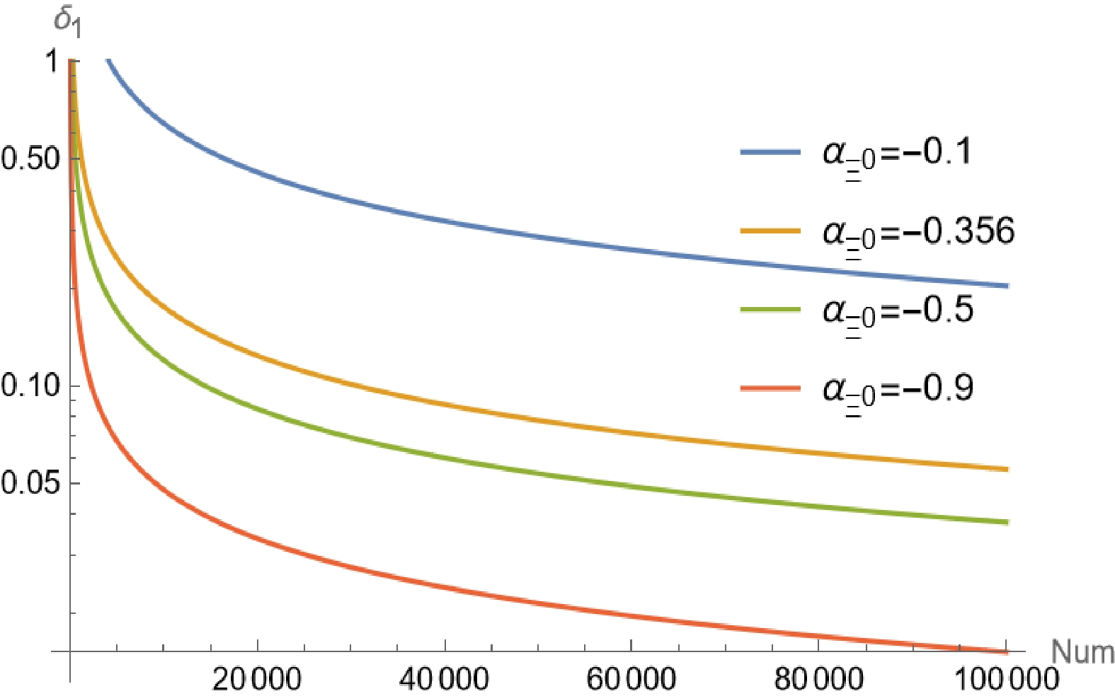
Figure 4. (color online) Sensitivity of
$ \alpha_{\Xi^0} $ relative to observed events N.
Figure 5. (color online) Sensitivity of
$ \alpha_{{\bar{\Xi}}^0} $ relative to observed events N. -
By examining the cascaded
$ J/\psi\to\Xi^0 {\bar{\Xi}}^0 $ ,$ \Xi^0\to\Lambda \pi^0 $ , and$ {\bar{\Xi}}^0\to{\bar{\Lambda}} \gamma $ decays, we derived formulae for angular distribution and observable quantities of polarization. They can be used to measure the Ξ decay asymmetric parameter in future experiments. Specifically, we estimated the statistical sensitivity of these parameters by considering the whole decay chain. According to the estimation results, even a large asymmetric parameter value requires more than 100,000 data events to realize a measurement accuracy of 1%. -
The helicity amplitudes can be expressed in the form of a complex number as follows:
$ \begin{array}{*{20}{l}} A^J_{\text{λ}_1,\text{λ}_2}=a^J_{\text{λ}_1,\text{λ}_2} {\rm e}^{{\rm i}\xi_{\text{λ}_1,\text{λ}_2}}, \end{array}\tag{A1} $

1. Expressions of real multipole parameters
$ Q^1_{i,j} $ $ \begin{aligned}[b] Q^{1}_{0,0} =& a_{\frac{1}{2},\frac{1}{2}}^2 \sin ^2\theta _0+\frac{1}{4} a_{\frac{1}{2},-\frac{1}{2}}^2 (\cos 2 \theta _0+3),\\ Q^{1}_{0,0}Q^{1}_{0,2} =& -\frac{a_{\frac{1}{2},-\frac{1}{2}} a_{\frac{1}{2},\frac{1}{2}} \sin 2 \theta _0\sin \Delta _a}{\sqrt{2}},\\ Q^{1}_{0,0}Q^{1}_{1,1} =& \frac{1}{2} (2 a_{\frac{1}{2},\frac{1}{2}}^2+a_{\frac{1}{2},-\frac{1}{2}}^2)\sin ^2\theta _0,\\ Q^{1}_{0,0}Q^{1}_{1,3} =& \frac{a_{\frac{1}{2},-\frac{1}{2}} a_{\frac{1}{2},\frac{1}{2}} \sin 2 \theta _0\cos \Delta _a}{\sqrt{2}},\\ Q^{1}_{0,0}Q^{1}_{2,0} =&\frac{a_{\frac{1}{2},-\frac{1}{2}} a_{\frac{1}{2},\frac{1}{2}} \sin 2 \theta _0\sin \Delta _a}{\sqrt{2}},\\ Q^{1}_{0,0}Q^{1}_{2,2} =& \frac{1}{2} (a_{\frac{1}{2},-\frac{1}{2}}^2-2 a_{\frac{1}{2},\frac{1}{2}}^2)\sin ^2\theta _0,\\ Q^{1}_{0,0}Q^{1}_{3,1} =& -\frac{a_{\frac{1}{2},-\frac{1}{2}} a_{\frac{1}{2},\frac{1}{2}} \sin 2 \theta _0\cos \Delta _a}{\sqrt{2}},\\ Q^{1}_{0,0}Q^{1}_{3,3} =&a_{\frac{1}{2},\frac{1}{2}}^2 \sin ^2\theta _0-\frac{1}{4} a_{\frac{1}{2},-\frac{1}{2}}^2 (\cos 2 \theta _0+3), \end{aligned}\tag{A2} $

and others are equal to zero.
2. The elements of
$ \rho^{\Lambda {\bar{\Lambda}}} $ $ \begin{aligned}[b] \rho^{\Lambda{\bar{\Lambda}}}_{\frac{1}{2}, \frac{1}{2}, \frac{1}{2},\frac{1}{2}} =&Q^{1}_{0,0} \left(1+\alpha _{\Xi^0 }\right) \left(1-\alpha _{{\bar{\Xi }}^0}\right)\\ &\times \big\{Q^{1}_{0,2} \sin \theta _2 \sin \phi _2+Q^{1}_{2,0} \sin \theta _1 \sin \phi _1\\ & +Q^{1}_{2,2} \sin \theta _1 \sin \theta _2 \sin \phi _1 \sin \phi _2\\ &+Q^{1}_{1,1} \sin\theta _1 \sin \theta _2 \cos \phi _1 \cos \phi _2\\ &+Q^{1}_{1,3} \sin \theta _1 \cos \theta _2 \cos \phi _1\\ &+Q^{1}_{3,1} \sin \theta _2 \cos \theta _1 \cos \phi _2\\ &+Q^{1}_{3,3} \cos \theta _1 \cos \theta _2+1\big\}, \end{aligned} $

$ \begin{aligned}[b] \rho^{\Lambda{\bar{\Lambda}}}_{\frac{1}{2}, \frac{1}{2}, -\frac{1}{2},\frac{1}{2}} =&Q^{1}_{0,0} \sqrt{1-\alpha _{\Xi^0 }^2} e^{-i \Delta _b} (1-\alpha _{{\bar{\Xi }}^0})\\ & \times \big\{Q^{1}_{1,1} \sin \theta _2 \cos \phi _2 (\cos \theta _1 \cos \phi _1\\ & +i \sin \phi _1)+Q^{1}_{1,3} \cos \theta _2 (\cos \theta _1 \cos \phi _1\\ & +i \sin \phi _1)+Q^{1}_{2,0} \cos \theta _1 \sin \phi _1\\ & -i Q^{1}_{2,2} \sin \theta _2 \sin \phi _2 \cos \phi _1\\ & +Q^{1}_{2,2} \sin \theta _2 \cos \theta _1 \sin \phi _1 \sin \phi _2\\ &-Q^{1}_{3,1} \sin \theta _1 \sin \theta _2 \cos \phi _2\\ & -Q^{1}_{3,3} \sin \theta _1 \cos \theta _2-i Q^{1}_{2,0} \cos \phi _1\big\}, \end{aligned} $

$ \begin{aligned}[b] \rho^{\Lambda{\bar{\Lambda}}}_{\frac{1}{2}, -\frac{1}{2}, \frac{1}{2},-\frac{1}{2}} =&-Q^{1}_{0,0} \left(1+\alpha _{\Xi^0 }\right) \left(1+\alpha _{{\bar{\Xi }}^0}\right) \\ &\times\big\{-1+Q^{1}_{0,2} \sin \theta _2 \sin \phi _2 \\&-Q^{1}_{2,0} \sin \theta _1 \sin \phi _1\\ & +Q^{1}_{2,2} \sin \theta _1 \sin \theta _2 \sin \phi _1 \sin \phi _2\\ &+Q^{1}_{1,1} \sin \theta _1 \sin \theta _2 \cos \phi _1 \cos \phi _2\\ & +Q^{1}_{1,3} \sin \theta _1 \cos \theta _2 \cos \phi _1\\ & +Q^{1}_{3,1} \sin \theta _2 \cos \theta _1 \cos \phi _2\\ & +Q^{1}_{3,3} \cos \theta _1 \cos \theta _2\big\}, \end{aligned} $

$ \begin{aligned}[b] \rho^{\Lambda{\bar{\Lambda}}}_{\frac{1}{2}, -\frac{1}{2}, -\frac{1}{2},-\frac{1}{2}} =&-Q^{1}_{0,0} \sqrt{1-\alpha _{\Xi^0 }^2} {\rm e}^{-{\rm i} \Delta _b} \left(\alpha _{{\bar{\Xi }}^0}+1\right) \\ & \times\big\{Q^{1}_{1,1} \sin \theta _2 \cos \phi _2 (\cos \theta _1 \cos \phi _1\\ & +i \sin \phi _1)+Q^{1}_{1,3} \cos \theta _2 (\cos \theta _1 \cos \phi _1 \\ & +i \sin \phi _1)-Q^{1}_{2,0} \cos \theta _1 \sin \phi _1\\ & -i Q^{1}_{2,2} \sin \theta _2 \sin \phi _2 \cos \phi _1\\ & +Q^{1}_{2,2} \sin \theta _2 \cos \theta _1 \sin \phi _1 \sin \phi _2\\ &-Q^{1}_{3,1} \sin \theta _1 \sin \theta _2 \cos \phi _2\\ & -Q^{1}_{3,3} \sin \theta _1 \cos \theta _2+i Q^{1}_{2,0} \cos \phi _1\big\}, \end{aligned} $

$ \begin{aligned}[b] \rho^{\Lambda{\bar{\Lambda}}}_{-\frac{1}{2}, \frac{1}{2}, \frac{1}{2},\frac{1}{2}} =&Q^{1}_{0,0} \sqrt{1-\alpha _{\Xi^0}^2} {\rm e}^{ {\rm i} \Delta _b} \left(1-\alpha _{{\bar{\Xi }}^0}\right)\\ & \times \big\{Q^{1}_{1,1} \sin \theta _2 \cos \phi _2 (\cos \theta _1 \cos \phi _1\\ & -i \sin \phi _1)+Q^{1}_{1,3} \cos \theta _2 (\cos \theta _1 \cos \phi _1 \\ & -i \sin \phi _1)+Q^{1}_{2,0} \cos \theta _1 \sin \phi _1\\ & +i Q^{1}_{2,2} \sin \theta _2 \sin \phi _2 \cos \phi _1\\ &+Q^{1}_{2,2} \sin \theta _2 \cos \theta _1 \sin \phi _1 \sin \phi _2\\ & -Q^{1}_{3,1} \sin \theta _1 \sin \theta _2 \cos \phi _2\\ & -Q^{1}_{3,3} \sin \theta _1 \cos \theta _2+i Q^{1}_{2,0} \cos \phi _1\big\}, \end{aligned} $

$ \begin{aligned}[b] \rho^{\Lambda{\bar{\Lambda}}}_{-\frac{1}{2}, \frac{1}{2}, -\frac{1}{2},\frac{1}{2}} =&Q^{1}_{0,0} \left(1-\alpha _{\Xi^0 }\right) \left(1-\alpha _{{\bar{\Xi }}^0}\right)\\ &\times \big\{1+Q^{1}_{0,2} \sin \theta _2 \sin \phi _2\\ & -Q^{1}_{2,0} \sin \theta _1 \sin \phi _1\\ & -Q^{1}_{2,2} \sin \theta _1 \sin \theta _2 \sin \phi _1 \sin \phi _2\\ & -Q^{1}_{1,1} \sin \theta _1 \sin \theta _2 \cos \phi _1 \cos \phi _2\\ &-Q^{1}_{1,3} \sin \theta _1 \cos \theta _2 \cos \phi _1\\ & -Q^{1}_{3,1} \sin \theta _2 \cos \theta _1 \cos \phi _2\\ &-Q^{1}_{3,3} \cos \theta _1 \cos \theta _2\big\}, \end{aligned} $

$ \begin{aligned}[b] \rho^{\Lambda{\bar{\Lambda}}}_{-\frac{1}{2}, -\frac{1}{2}, \frac{1}{2},-\frac{1}{2}} =&-Q^{1}_{0,0} \sqrt{1-\alpha _{\Xi^0 }^2} {\rm e}^{ {\rm i} \Delta _b} \left(\alpha _{{\bar{\Xi }}^0}+1\right)\\ & \times \big\{Q^{1}_{1,1} \sin \theta _2 \cos \phi _2 (\cos \theta _1 \cos \phi _1\\ & -i \sin \phi _1)+Q^{1}_{1,3} \cos \theta _2 (\cos \theta _1 \cos \phi _1\\ & -i \sin \phi _1)-Q^{1}_{2,0} \cos \theta _1 \sin \phi _1\\ &+i Q^{1}_{2,2} \sin \theta _2 \sin \phi _2 \cos \phi _1\\ & +Q^{1}_{2,2} \sin \theta _2 \cos \theta _1 \sin \phi _1 \sin \phi _2\\ &-Q^{1}_{3,1} \sin \theta _1 \sin \theta _2 \cos \phi _2\\ & -Q^{1}_{3,3} \sin \theta _1 \cos \theta _2-i Q^{1}_{2,0} \cos \phi _1\big\}, \end{aligned} $

$ \begin{aligned}[b] \rho^{\Lambda{\bar{\Lambda}}}_{-\frac{1}{2}, -\frac{1}{2}, -\frac{1}{2},-\frac{1}{2}} =&Q^{1}_{0,0} \left(1-\alpha _{\Xi^0 }\right)\left(1+\alpha _{{\bar{\Xi }}^0}\right)\\ & \times \big\{1-Q^{1}_{0,2} \sin \theta _2 \sin \phi _2\\ & -Q^{1}_{2,0} \sin \theta _1 \sin \phi _1\\ & +Q^{1}_{2,2} \sin \theta _1 \sin \theta _2 \sin \phi _1 \sin \phi _2\\ &+Q^{1}_{1,1} \sin \theta _1 \sin \theta _2 \cos \phi _1 \cos \phi _2\\ &+Q^{1}_{1,3} \sin \theta _1 \cos \theta _2 \cos \phi _1\\ & +Q^{1}_{3,1} \sin \theta _2 \cos \theta _1 \cos \phi _2\\ &+Q^{1}_{3,3} \cos \theta _1 \cos \theta _2\big\},\\ \end{aligned} \tag{A3}$

and the unlisted elements are equal to zero.
3. Expressions of real multipole parameters
$ Q^2_{i,j} :$ $ \begin{aligned}[b] Q^{2}_{0,0} =&\frac{1}{4} Q^{1}_{0,0} \big\{1+Q^{1}_{2,0} \alpha _{\Xi^0 } \sin \theta _1 \sin \phi _1\\ & +\alpha _{{\bar{\Xi }}^0} \big[-\alpha _{\Xi^0 } \big(Q^{1}_{1,1} \sin \theta _1 \sin \theta _2 \cos \phi _1 \cos \phi _2\\ & +Q^{1}_{1,3} \sin \theta _1 \cos \theta _2 \cos \phi _1 \\ & +\sin \theta _2 \big(Q^{1}_{2,2} \sin \theta _1 \sin \phi _1 \sin \phi _2\\ & +Q^{1}_{3,1} \cos \theta _1 \cos \phi _2\big)+Q^{1}_{3,3} \cos \theta _1 \cos \theta _2\big)\\ & -Q^{1}_{0,2} \sin \theta _2 \sin \phi _2\big]\big\}, \end{aligned} $

$ \begin{aligned}[b] Q^{2}_{0,0}Q^{2}_{0,3} =&\frac{1}{4} Q_{0,0} \big\{-\alpha _{{\bar{\Xi }}^0} (Q_{2,0} \alpha _{\Xi ^0} \sin \theta _1 \sin \phi _1+1)\\ & +\alpha _{\Xi^0} [Q_{2,2} \sin \theta _1 \sin \theta _2 \sin \phi _1 \sin \phi _2\\ & +Q_{1,1} \sin \theta _1 \sin \theta _2 \cos \phi _1 \cos \phi _2\\& +Q_{1,3} \sin \theta _1 \cos \theta _2 \cos \phi _1\\ & +Q_{3,1} \sin \theta _2 \cos \theta _1 \cos \phi _2+Q_{3,3} \cos \theta _1 \cos \theta _2]\\ & +Q_{0,2} \sin \theta _2 \sin \phi _2\big\}, \end{aligned} $

$\begin{aligned}[b] Q^{2}_{0,0}Q^{2}_{1,0} =&-\frac{1}{4} Q_{0,0} \sqrt{1-\alpha _{\Xi^0 }^2} \big\{\alpha _{{\bar{\Xi }}^0} [Q_{1,1} \sin \theta _2 \cos \phi _2\\ & \times (\cos \theta _1 \cos \phi _1 \cos \Delta _b+\sin \phi _1 \sin \Delta _b)\\ & +Q_{1,3} \cos \theta _2 (\cos \theta _1 \cos \phi _1 \cos \Delta _b\\ & +\sin \phi _1 \sin \Delta _b)+\sin \theta _2 (Q_{2,2} \sin \phi _2\\ & \times (\cos \theta _1 \sin \phi _1 \cos \Delta _b-\cos \phi _1 \sin \Delta _b)\\ & -Q_{3,1} \sin \theta _1 \cos \phi _2 \cos \Delta _b)\\ & -Q_{3,3} \sin \theta _1 \cos \theta _2 \cos \Delta _b]\\ & +Q_{2,0} (\cos \phi _1 \sin \Delta _b-\cos \theta _1 \sin \phi _1 \cos \Delta _b)\big\}, \end{aligned} $

$ \begin{aligned}[b] Q^{2}_{0,0}Q^{2}_{1,3} =&\frac{1}{4} Q^{1}_{0,0} \sqrt{1-\alpha _{\Xi^0 }^2} \big[-Q^{1}_{2,0} \cos \theta _1 \sin \phi _1 \alpha _{{\bar{\Xi }}^0} \\ & \times\cos \Delta _b+Q^{1}_{1,1} \sin \theta _2 \cos \phi _2 \\ & \times(\cos \theta _1 \cos \phi _1 \cos \Delta _b+\sin \phi _1 \sin \Delta _b)\\ & +Q^{1}_{1,3} \cos \theta _2 (\cos \theta _1 \cos \phi _1 \cos \Delta _b\\ &+\sin \phi _1 \sin \Delta _b)\\ & -Q^{1}_{2,2} \sin \theta _2 \sin \phi _2 \cos \phi _1 \sin \Delta _b\\ & +Q^{1}_{2,2} \sin \theta _2 \cos \theta _1 \sin \phi _1 \sin \phi _2 \cos \Delta _b\\ & -Q^{1}_{3,1} \sin \theta _1 \sin \theta _2 \cos \phi _2 \cos \Delta _b\\& +Q^{1}_{2,0} \cos \phi _1 \alpha _{{\bar{\Xi }}^0} \sin \Delta _b\\ & -Q^{1}_{3,3} \sin \theta _1 \cos \theta _2 \cos \Delta _b\big],\\ \end{aligned} $

$ \begin{aligned}[b] Q^{2}_{0,0}Q^{2}_{2,0} =&\frac{1}{4} Q^{1}_{0,0} \sqrt{1-\alpha _{\Xi ^0}^2} \big\{\alpha _{{\bar{\Xi }}^0} \big[Q^{1}_{1,1} \sin \theta _2 \cos \phi _2 \\ & \times(\sin \phi _1 \cos \Delta _b-\cos \theta _1 \cos \phi _1 \sin \Delta _b)\\ &+Q^{1}_{1,3} \cos \theta _2 (\sin \phi _1 \cos \Delta _b\\ & -\cos \theta _1 \cos \phi _1 \sin \Delta _b)+\sin \theta _2 (-Q^{1}_{2,2} \sin \phi _2\\ & \times (\cos \theta _1 \sin \phi _1 \sin \Delta _b+\cos \phi _1 \cos \Delta _b)\\ & +Q^{1}_{3,1} \sin \theta _1 \cos \phi _2 \sin \Delta _b)\\ &+Q^{1}_{3,3} \sin \theta _1 \cos \theta _2 \sin \Delta _b\big]\\ & +Q^{1}_{2,0} (\cos \theta _1 \sin \phi _1 \sin \Delta _b+\cos \phi _1 \cos \Delta _b)\big\}, \end{aligned} $

$ \begin{aligned}[b] Q^{2}_{0,0}Q^{2}_{2,3} =&\frac{1}{4} Q^{1}_{0,0} \sqrt{1-\alpha _{\Xi ^0}^2} \big[-Q^{1}_{2,0} \cos \theta _1 \sin \phi _1 \alpha _{{\bar{\Xi }}^0} \\ & \times\sin \Delta _b-Q^{1}_{2,0} \cos \phi _1 \alpha _{{\bar{\Xi }}^0} \cos \Delta _b\\ & +Q^{1}_{1,1} \sin \theta _2 \cos \phi _2 (\cos \theta _1 \cos \phi _1 \sin \Delta _b\\ & -\sin \phi _1 \cos \Delta _b)+Q^{1}_{1,3} \cos \theta _2 (\cos \theta _1 \cos \phi _1\\ & \times \sin \Delta _b-\sin \phi _1 \cos \Delta _b)+Q^{1}_{2,2} \sin \theta _2 \\ & \times\sin \phi _2 \cos \phi _1 \cos \Delta _b+Q^{1}_{2,2} \sin \theta _2 \cos \theta _1 \end{aligned} $

$ \begin{aligned}[b] & \times\sin \phi _1 \sin \phi _2 \sin \Delta _b-Q^{1}_{3,1} \sin \theta _1 \sin \theta _2\\ & \times \cos \phi _2 \sin \Delta _b-Q^{1}_{3,3} \sin \theta _1 \cos \theta _2 \sin \Delta _b\big],\\ Q^{2}_{0,0}Q^{2}_{3,0} =&\frac{1}{4} Q^{1}_{0,0} \big\{\alpha _{\Xi ^0} \left(1-Q^{1}_{0,2} \sin \theta _2 \sin \phi _2 \alpha _{{\bar{\Xi }}^0}\right)\\ & -\alpha _{{\bar{\Xi }}^0} [Q^{1}_{1,1} \sin \theta _1 \sin \theta _2 \cos \phi _1 \cos \phi _2\\ &+Q^{1}_{1,3} \sin \theta _1 \cos \theta _2 \cos \phi _1+\sin \theta _2 (Q^{1}_{2,2} \sin \theta _1\\ & \times \sin \phi _1 \sin \phi _2+Q^{1}_{3,1} \cos \theta _1 \cos \phi _2)\\ &+Q^{1}_{3,3} \cos \theta _1 \cos \theta _2]+Q^{1}_{2,0} \sin \theta _1 \sin \phi _1\big\},\\ Q^{2}_{0,0}Q^{2}_{3,3} =&\frac{1}{4} Q^{1}_{0,0} \big[-\alpha _{\Xi^0 } \left(\alpha _{{\bar{\Xi }}^0}-Q^{1}_{0,2} \sin \theta _2 \sin \phi _2\right)\\ & -Q^{1}_{2,0} \sin \theta _1 \sin \phi _1 \alpha _{{\bar{\Xi }}^0}+Q^{1}_{2,2} \sin \theta _1 \sin \theta _2\\ & \times \sin \phi _1 \sin \phi _2+Q^{1}_{1,1} \sin \theta _1 \sin \theta _2 \cos \phi _1 \cos \phi _2\\ & +Q^{1}_{1,3} \sin \theta _1 \cos \theta _2 \cos \phi _1+Q^{1}_{3,1} \sin \theta _2 \cos \theta _1\\ & \times \cos \phi _2+Q^{1}_{3,3} \cos \theta _1 \cos \theta _2\big], \end{aligned}\tag{A4} $

and other parameters are equal to zero.
Phenomenological study of ${{{J/\psi\to\Xi^0(\Lambda \pi^0) {\bar{\Xi}}^0({\bar{\Lambda}} \gamma)}}}$ decays
- Received Date: 2023-03-20
- Available Online: 2023-09-15
Abstract: The measurement of decay parameters is one of the important goals of particle physics experiments, and the measurement serves as a probe to search for evidence of CP violation in baryonic decays. The experimental results will aid in advancing existing theoretical research and establishing new experimental objectives. In this study, we formulate the asymmetric parameters that characterize parity violation, and then derive formulas for the measurement of CP violation. The formulae for the joint angular distribution of the full decay chain as well as the polarization observable of


 DownLoad: