


 Abstract
 HTML
HTML Reference
 Related
 PDF
PDF


-
The 4321 model [1−5] is an ultraviolet-complete model that extends the standard model (SM) gauge groups to a larger
${S U}(4) \times {S U}(3)' \times {S U}(2)_L \times {U}(1)'$ group. It is motivated by recent measurements of B hadron decays that are in tension [1] with the SM and can provide a combined explanation for multiple anomalies observed in b hadron decays, which point to lepton flavor nonuniversality. This model also provides a novel and interesting final state topology to search for at colliders, with multi-jets and multi-tau leptons. A search for pair production of the lightest new particles in this model, such as vector-like leptons (VLLs), was recently performed [6] at the CMS experiment based on data collected in 2017 and 2018 corresponding to a total integrated luminosity of 96.5${ \mathrm{fb^{-1}}}$ . Interestingly, a mild excess has been found at the level of 2.8 standard deviations for a representative VLL mass point of 600 GeV [6]. In this study, we perform a similar investigation on a future TeV-scale muon collider [7], which should have great potential to explore VLLs and other predicted new particles in the 4321 model to a large extent.A muon-muon collider with a center-of-mass energy at the multi-TeV scale has recently received much-revived interest [7] and has several advantages over both hadron-hadron and electron–electron colliders [8−10]. Because massive muons emit considerably less synchrotron radiation than electron beams, muons can be accelerated in a circular collider to higher energies with a much smaller circumference. Moreover, because the proton is a composite particle, muon-muon collisions are cleaner than proton-proton collisions and thus can lead to higher effective center-of-mass energies. However, owing to the short lifetime of the muon, the beam-induced background (BIB) from muon decays must be examined and properly reduced. Based on a realistic simulation at
$ \sqrt{s}=1.5 $ TeV with BIB included, Ref. [11] found that the coupling between the Higgs boson and the b-quark can be measured at percent level with order${\mathrm{ab^{-1}}}$ of collected data. -
The 4321 model includes the existence of new massive bosons and fermions. It features a massive vector leptoquark, U, which couples both to leptons and quarks. To be UV complete and maintain agreement with other measurements, the 4321 model contains two other sets of bosons and families of vector-like fermions. In the 4321 model, VLLs come in electroweak doublets with one charged VLL,
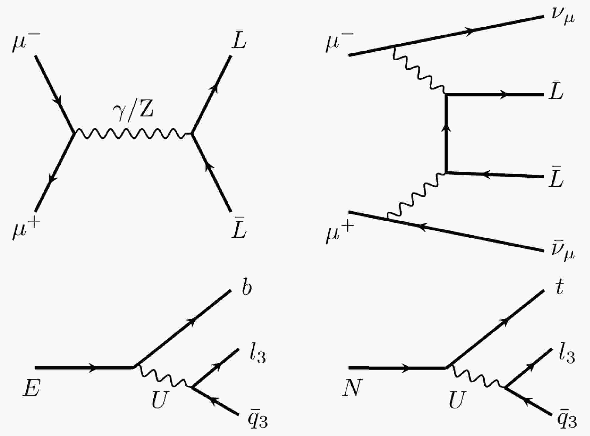
${E}$ , and one neutral VLL,${ N }$ , whose masses are taken to be equal. The VLLs may be produced via electroweak production through their couplings to the SM${ W }$ and${ Z }$ /γ bosons or via interactions with a new heavy${Z}^\prime$ boson introduced by the 4321 model. In this study, we consider only the electroweak production and ignore potential contributions from the${Z}^\prime$ boson. Examples of Feynman diagrams showing VLL pair production through a) s-channel ($\mu^+\mu^-\rightarrow { {L}} { {L}}$ , where${ L }$ represents either${ N }$ or${ E }$ ) and b) vector boson scattering (VBS) at a TeV muon collider ($\mu^+\mu^-\rightarrow L L \nu_\mu\bar{\nu}_\mu$ ), as well as diagrams of the VLL decays, are shown in Fig. 1. The VLLs decay via a virtual leptoquark, U, to two quarks and one lepton. The leptoquark is expected to couple most strongly to the third generation to explain the B anomalies. For each second- and first-generation fermion, suppression of one or more orders of magnitude in the branching fraction is expected. We consider only the dominant decays, that is, decays to third-generation fermions.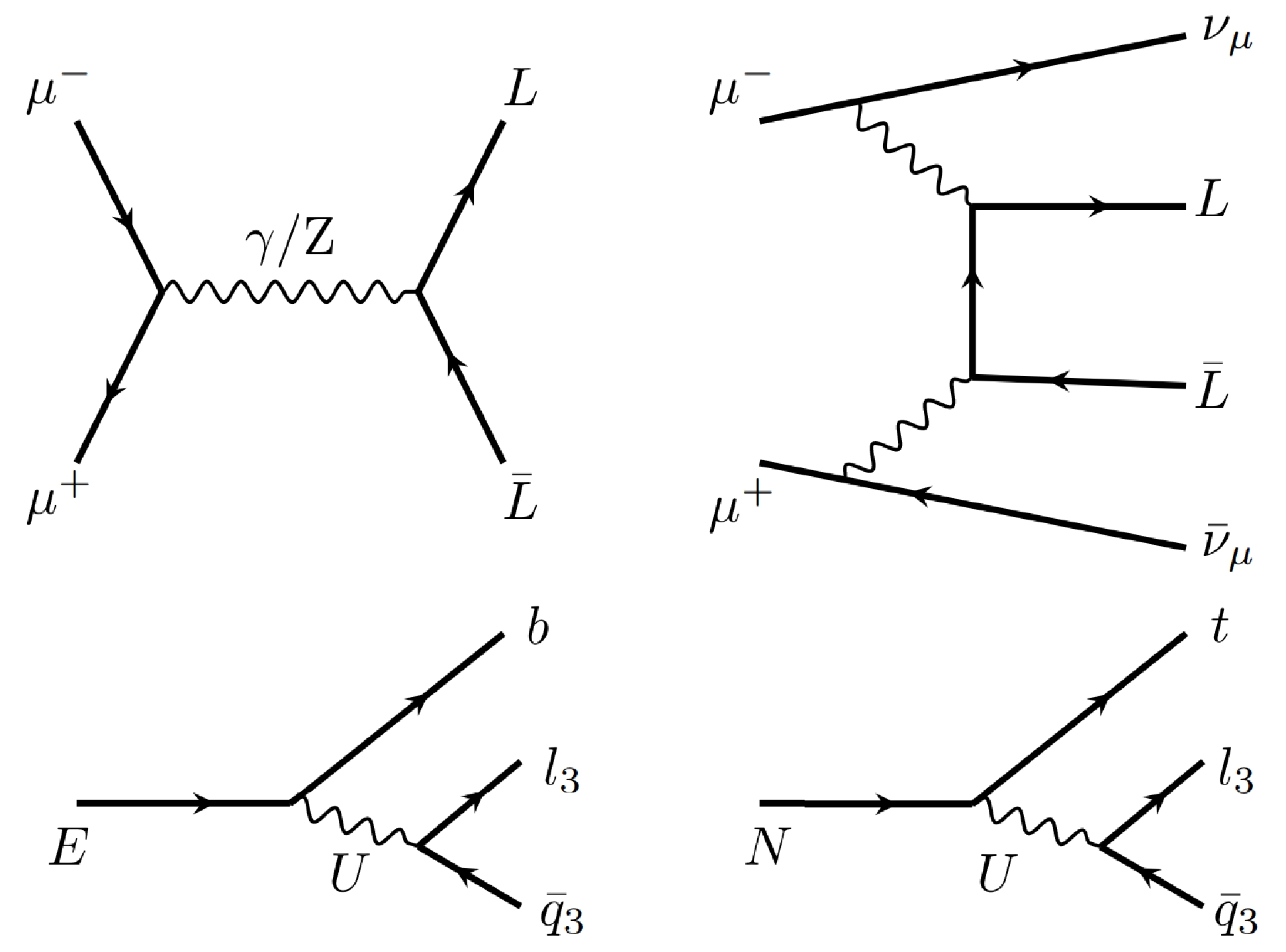
Figure 1. Top side: Example Feynman diagrams showing VLL pair production through s-channel and vector boson scattering at a TeV muon collider.
${L}$ represents either the neutral VLL,${N}$ , or the charged VLL,${E}$ . Bottom side: Vector-like lepton decays are mediated by a vector leptoquark, U. These decays are primarily to third-generation leptons and quarks.Figure 2 shows the cross sections of various processes and VLL mass points at the center-of-mass energy
$ \sqrt{s}=3 $ or 10 TeV. The cross sections of the EE processes are larger than those of the NN processes by one order of magnitude. The VBS cross sections are smaller by several orders of magnitude than those of pair production. Hence, we hereafter focus on the EE pair production processes.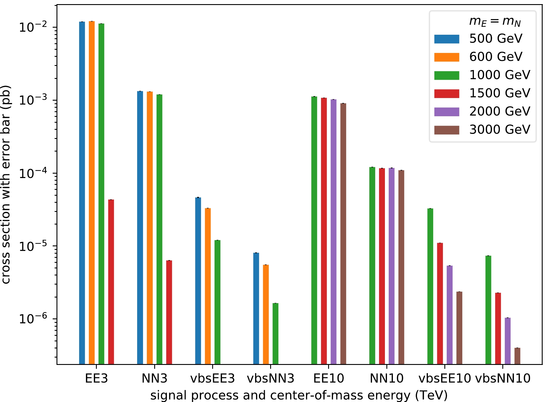
Figure 2. (color online) Cross sections of various signal processes and VLL mass points in two benchmark collider proposals with
$ \sqrt{s}=3 $ or 10 TeV. The x-axis shows the process symbol (pair production,$\mu^+\mu^-\rightarrow LL$ , or VBS production,$\mu^+\mu^-\rightarrow LL \nu_\mu\bar{\nu}_\mu$ ) and$ \sqrt{s} $ in the scale of$ \mathrm{TeV} $ , whereas the y-axis on the logarithmic scale indicates the cross sections in units of$ \mathrm{pb} $ . The cross sections of$ m_E = m_N = $ 1500 GeV are non-vanishing owing to the offshell E, N. The VBS processes with$ m_E = m_N = 1500\ \mathrm{GeV} $ and$ \sqrt{s}=3 $ TeV result in negligible cross sections.The background processes we consider include
● b1)
$ \mu^+\mu^-\rightarrow b\bar{b}\,, b\bar{b}Z $ ,● b2)
$ \mu^+\mu^-\rightarrow \tau^+\tau^-\,, \tau^+\tau^-Z $ ,● b3)
$ \mu^+\mu^-\rightarrow W^+W^-\,, W^+W^-Z $ ,● b4)
$ \mu^+\mu^-\rightarrow t\bar{t}\,, t\bar{t}Z $ ,● b5)
$ \mu^+\mu^-\rightarrow ZZh\,, Zhh\,, t\bar{t}h\,, bbh\,, WWh\,, \tau^+\tau^-h $ (collectively named “others”),● b6) VBS production of
$ b\bar{b}\,,\tau^+\tau^-\,,W^+W^-\,,t\bar{t} $ . -
We consider the muon collider benchmarks in which
$ \sqrt{s}=3 $ TeV and L = ab$ ^{-1} $ in this study. Both signal and background events are simulated with MadGraph5_aMC@NLO and then showered and hadronized by Pythia8 [12]. The final state jets are clustered using fastjet [13] with the VLC [14, 15] algorithm at a fixed cone size of$ R_{\rm jet}=0.5 $ . We use delphes [16] 3.5.0 to simulate detector effects with the newly-added card for the muon collider detector [17]. The jet flavor tagging efficiencies are listed in Table 1. However, note that jet tagging techniques for muon colliders are currently in their preliminary stage [11, 18] and have a large potential for improvement.Flavor Tagged as light Tagged as b light 0.9 0.01 b 0.1 0.7 Table 1. Flavor tagging efficiencies used in this analysis.
The hadronic τ identification efficiency is chosen from the performance of the CMS detector. The mis-tagging rates are both
$ \sim1 $ % from CEPC detector simulation [19] and CMS estimation [20].Figure 3 shows signal and stacked background distributions on the multiplicities of identified tau, b-jet, and additional leptons, simulated at a 3 TeV muon collider. We can see that pair production of EE processes have dominant significance. Based on the optimization performance shown in Fig. 3, we define our preselection criteria as follows: events must include at least a pair of identified opposite sign τs, 3 b-tagged jets, while events with additional leptons are vetoed. The selection efficiency of background/signal events before any cuts and after the preselection cuts is shown in Table 2.
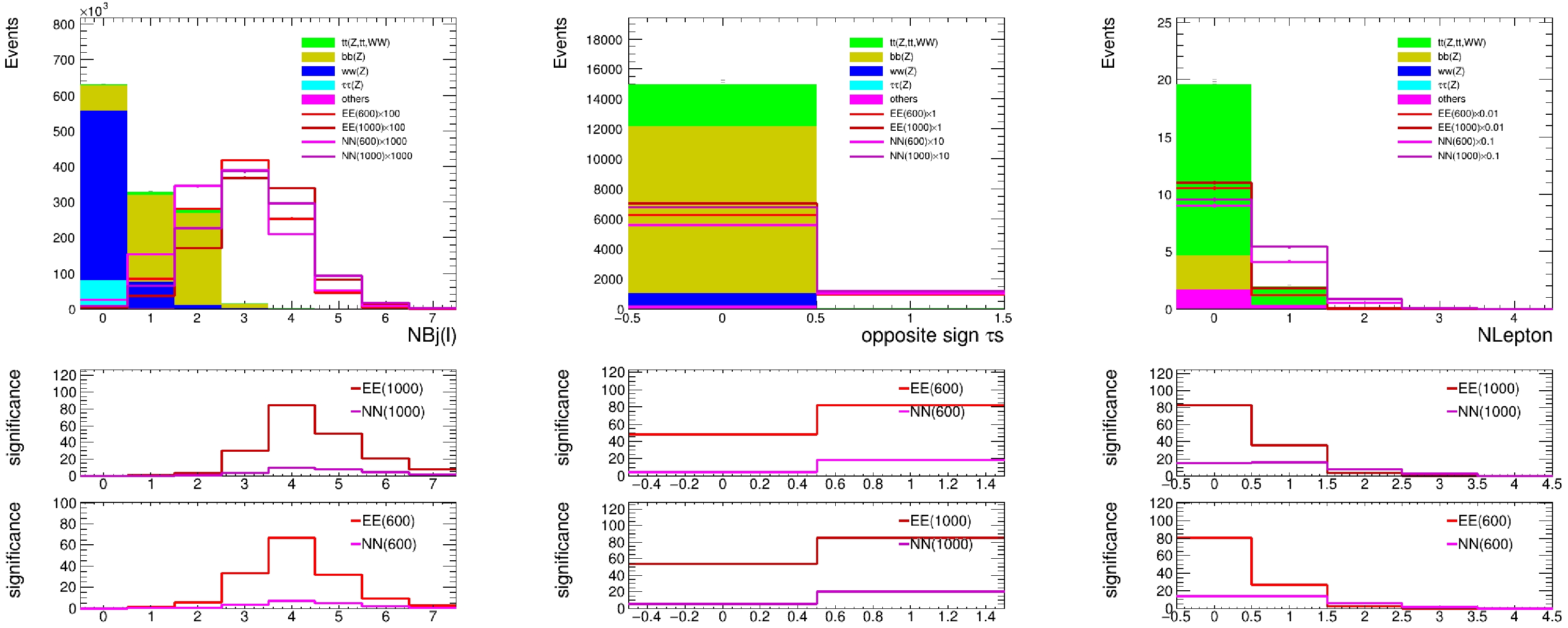
Figure 3. (color online) Signal and stacked background distributions on the multiplicities of identified b-jet, tau (requiring 3 b-tagged jets in events), and additional leptons (requiring 3 b-tagged jets in events and no additional leptons in the events), simulated at a 3 TeV muon muon collider. The ratio plots below show the statistic only significance estimated for each signal point, based on which we can decide on selections with the best performance.
Efficiency Background Signal Preselection 0.0017% 9.6% Table 2. Selection efficiency of background/signal events before any cuts and after the preselection cuts.
-
The reconstruction of the VLL candidates starts with selecting and clustering five or six jets into two reconstructed VLLs using the following algorithm looping through a maximum of ten jets:
● Select 2 τ jets and 4 b-tagged jets (for events with only 3 b tagged jets, a jet is selected or zero padding is applied, if there is no jet expect the jets already considered) as b candidates.
● Construct the combinatorics of the 2 τ and 4 b candidates into (
$ {\tau}_1,b_1,b_2 $ ),($ {\tau}_2,b_3,b_4 $ ).● Calculate the invariant mass of the systems (
$ {\tau}_1,b_1,b_2 $ ) and ($ {\tau}_2,b_3,b_4 $ ), denoted as$ M({\tau}_1,b_1,b_2) $ and$ M({\tau}_2,b_3,b_4) $ , respectively.● Calculate
$ \Delta M^2=M({\tau}_1,b_1,b_2)^2-M({\tau}_2,b_3,b_4)^2 $ ,● (
$ {\tau}_1,b_1,b_2 $ ) and ($ {\tau}_2,b_3,b_4 $ ) giving the lowest$ \Delta M^2 $ are reconstructed as 2 VLLs.Additional pairs of VLLs are reconstructed by requiring a relatively small
$ \Delta M^2 $ . This algorithm is used to construct the input for BDT training. -
To implement the BDT, we shuffle the signal and background events and define the training and test sets with an event ratio of
$ 4:1 $ . A BDT with 850 trees and a maximum depth of three is trained. We apply the per-event weight during training to account for the cross-section difference among the background processes. The weight is defined by$ \begin{equation} n_{L_X}=\sigma_XL/N_{G_X}, \end{equation} $

(1) where
$ \sigma_X $ denotes the cross-section of a process, L denotes the default target luminosity in this study at approximately 1${ \mathrm{ab^{-1}}}$ for a 3 TeV muon collider, and$ N_{G_X} $ denotes the generated number of events. The total signal yields are reweighted to match those of the total background during training for the robustness of the trained model. Signal yields corresponding to different VLL masses are weighted to be the same. The input features, namely, the reconstructed kinematics of each event used in training, are listed as follows and summarized in Table 3:Objective Features Number of features Each jet $ ({p_\mathrm{T}},\,\eta,\,\phi,mass,flavor) $ 

50 ${\not{E}}$ 

$ ({p_\mathrm{T}},\,\eta,\,\phi) $ 

3 Each pair of VLL candidates $ ({p_\mathrm{T}},\,\eta,\,\phi,mass,flavor,\Delta \phi,\,\Delta R) $ 

48 Total: 101 Table 3. Summary of features used for BDT training.
●
$ ({p_\mathrm{T}},\,\eta,\,\phi,\,mass) $ of a maximum of 10 jets including τs. τ jets are prior to b candidates, and both have higher priorities than rest jets.●
$ ({p_\mathrm{T}},\,\eta,\,\phi) $ of the missing energy${\not {E}}$ .●
$({p_\mathrm{T}},\, \eta,\; \phi, \; mass,\; Nb\, jets\; in\; VLL)$ of the six pairs of VLL candidates.●
$ (\Delta \phi,\,\Delta R) $ between each pair of VLLs candidates. -
Using the variables of jets and MET from the input of the BDT model, for each signal or background event, we have a flattened feature vector of size 53 to describe the information extracted from the final state. A direct way to construct a classifier based on the already vectorized input without any concise symmetry is to build fully-connected dense layers (simple fully-connected DNNs).
Because the input features are spread over many orders of magnitude, feature-wise normalization is performed before feeding the data into the network. Several architectures of simple fully-connected DNNs are tried, which share the same 53-neuron input layer and sigmoid-activated 1-neuron output layer, differing only in the number and size of the ReLU-activated hidden layers. The RMSProp optimizer with an initial learning rate of
$ 10^{-4} $ and a batch size of 32 is used to minimize the binary cross entropy loss. Training, validation, and test samples are randomly taken from the dataset following the$ 8:1:1 $ ratio, and the training samples are shuffled at the beginning of each epoch. Validation is performed at the end of each epoch. -
The ABCNet [21] is an attention-based graph neural network that takes advantage of the graph attention polling (GAP) [22] layers to enhance the local feature extraction, in addition to the previous state-of-the-art model ParticleNet [23], for tasks such as quark-gluon tagging and pileup mitigation. For the purpose of binary classification between the signal and background events in the context of the 4321 model in literature [6] and this paper, the model takes batches of the point-cloud encoded events as inputs and outputs the predicted probabilities for each event to be the signal, which we refer to as ABCNet scores in the following.
Specifically, point-cloud encoding contains both detailed information about jets (local features, including τ jets and b candidates) and about the entire event (global features). For each event, the cloud collects a maximum of 10 jets with their kinematics, charges, and b-tagging results. τ jets are prior to b candidates, and both are then sorted by
$p_T$ in descending order. Jets with lower priorities are discarded if more than 10 are found, and zero padding is applied to ensure 10 points to input otherwise. We summarize the local features in Table 4 and also provide the missing energy as global features. The two input categories of features are integrated by ABCNet to predict the ABCNet score. We cut the events as follows before building the dataset:No. Feature Description 0 η pseudorapidity of the jet momentum 1 ϕ azimuthal angle of the jet momentum 2 $\log\dfrac{p_T}{\mathrm{GeV} }$ 

transverse momentum of the jet, with logarithmic scaling 3 $ \log\dfrac{m}{\mathrm{GeV}} $ 

static mass of the jet, with logarithmic scaling 4 Q charge for a τ jet or zero filling otherwise 5 $ \mathrm{BTag}_{50} $ 

b-tagging result for a b candidate with $ \epsilon_\mathrm s = 50$ % or zero filling otherwise

6 $ \mathrm{BTag}_{70} $ 

b-tagging result for a b candidate with $ \epsilon_\mathrm s = 70$ % or zero filling otherwise

7 $ \mathrm{BTag}_{90} $ 

b-tagging result for a b candidate with $ \epsilon_\mathrm s = 90$ % or zero filling otherwise

Table 4. Input local features of our ABCNet model.
● At least 3 b-tagged candidates with
$ \epsilon_\mathrm s = 90$ % ;● At least 2 τ, with at least 1
$ \tau^+ $ and at least 1$ \tau^- $ ;● No lepton.
Then, the events are shuffled and split into training, validation, and test sets with the
$ 8:1:1 $ ratio.Our ABCNet model is similar to that used by the CMS collaboration [6], except for the three input global features and the fully connected layer of size 16 connecting them to the aggregation. It is tuned, starting from Fig. 1 in literature [21], shrinking the edge size of the first GAP block to 16, decreasing the capacities of the layers immediately after the two GAPs block both to 64, and replacing the structures after the aggregation to two fully connected layers of size 256, sandwiching a max-polling layer before the softmax activated output layer of size 2. In addition, to avoid over-training, we apply a dropout after each hidden fully connected layer, whose ratio is tuned to be 0.3. Figure 4 shows the architecture of the ABCNet used in this study. We use the Adam optimizer with a batch size of 64 and a learning rate decaying exponentially from
$ 10^{-2} $ , which performs well both in feature extraction and over-fit avoidance. We monitor the training process with metric validation accuracy and perform an early stop if the metric value does not improve over the nearest 10 epochs. The best-fit model with the highest validation accuracy is then tested over the test set to ensure accuracy and conduct AUC evaluation.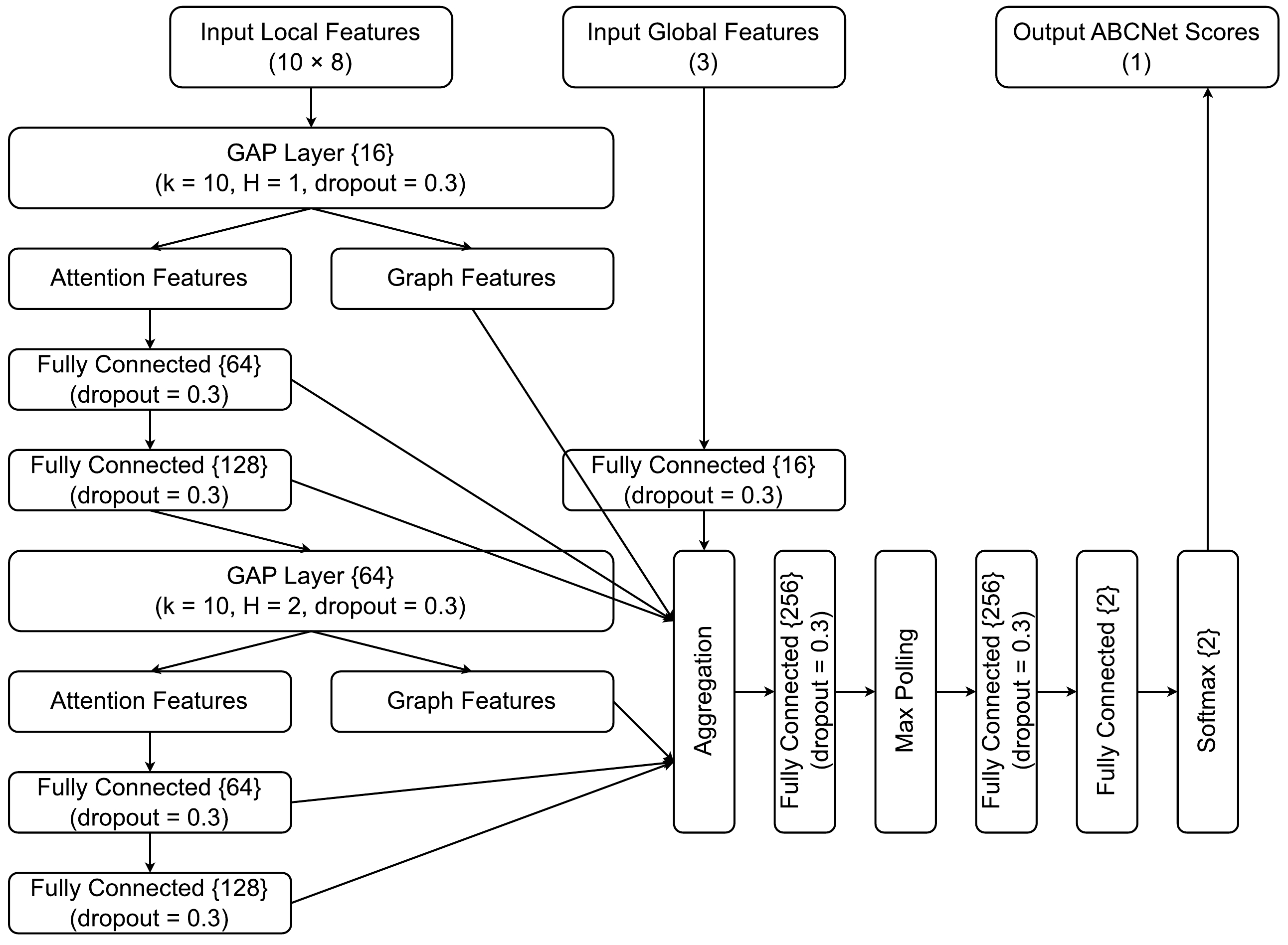
Figure 4. ABCNet architecture used in this study.
Owing to the insufficiency of MC samples originating from the slowness of simulation, as well as our intention to use the entire dataset to set limits afterward, we equally divide the set into 10 folds for cross-validation. For each fold, the model is trained on other folds and tested on the unseen fold to give ABCNet scores. Figure 5 (a) visualizes the distribution of the ABCNet scores in the 10 mutually exclusive test folds. For both the signal and background events, their distributions do not vary much between different folds, although the signal and background distributions do separate to a large extent. The two features show the excellent generalizing and distinguishing powers of the model. To further inspect the stability and generalization of the model, Table 5 gives the detailed performance of the model over the 10 different folds and the overall values. For each of the 10 runs, we perform the Kolmogorov-Smirnov test to ensure that no over-fitting occurs with respect to the correspondence of the ABCNet score distributions over the training and test sets for both signal and background samples, among which the result of the first run is visualized in Fig. 5 (b).
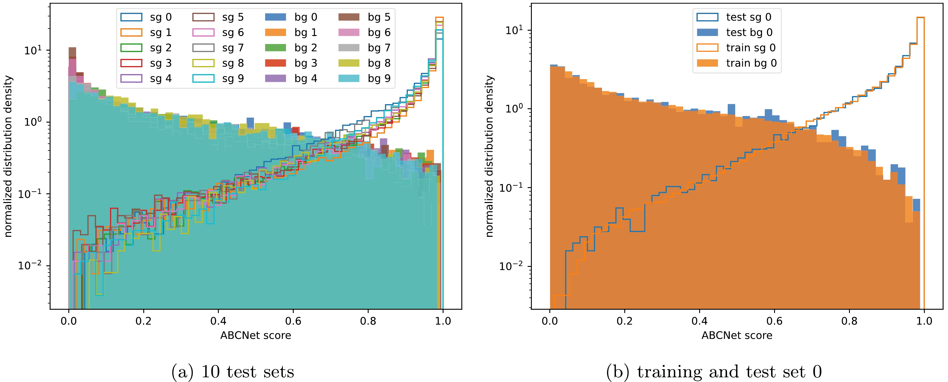
Figure 5. (color online) (a) ABCNet score distribution histogram of the signal (sg) and background (bg) events from 10 mutually exclusive data folds. (b) ABCNet score distributions over the training and test sets during the first round (round 0) of the 10-fold cross-validation.
No. Accuracy AUC S p-value B p-value 0 0.9305 0.9660 0.5349 0.1672 1 0.9365 0.9726 0.0130 0.7574 2 0.9373 0.9707 0.4207 0.2046 3 0.9362 0.9698 0.5278 0.0541 4 0.9331 0.9671 0.3081 0.0281 5 0.9362 0.9715 0.8091 0.0389 6 0.9420 0.9744 0.3776 0.2883 7 0.9358 0.9687 0.3732 0.4290 8 0.9399 0.9734 0.7797 0.1458 9 0.9352 0.9686 0.7758 0.5006 mean 0.9363 0.9703 0.4920 0.2614 std 0.0030 0.0026 0.2372 0.2246 overall 0.9363 0.9698 - - Table 5. Performance of the ABCNet model over the 10 different folds and the overall values. In the table, std denotes the standard deviation, and S and B denote signal and background, respectively. The overall AUC is computed by gathering the 10 folds to evaluate the overall FPR and TPR and are thus slightly variant from the mean value of the group.
-
Receiver operating characteristic (ROC) curves are shown in Fig. 6 to illustrate the performance of the classifiers. Our primary metric for comparison is the area under the ROC curve (AUC), with a higher AUC value indicating a more robust classification power across a wide range of working points. This metric is insightful because it is directly connected to classification accuracy, the quantity optimized in hyperparameter tuning, and other important metrics. The statistical significance is calculated to reveal its strong positive dependence on the AUC.
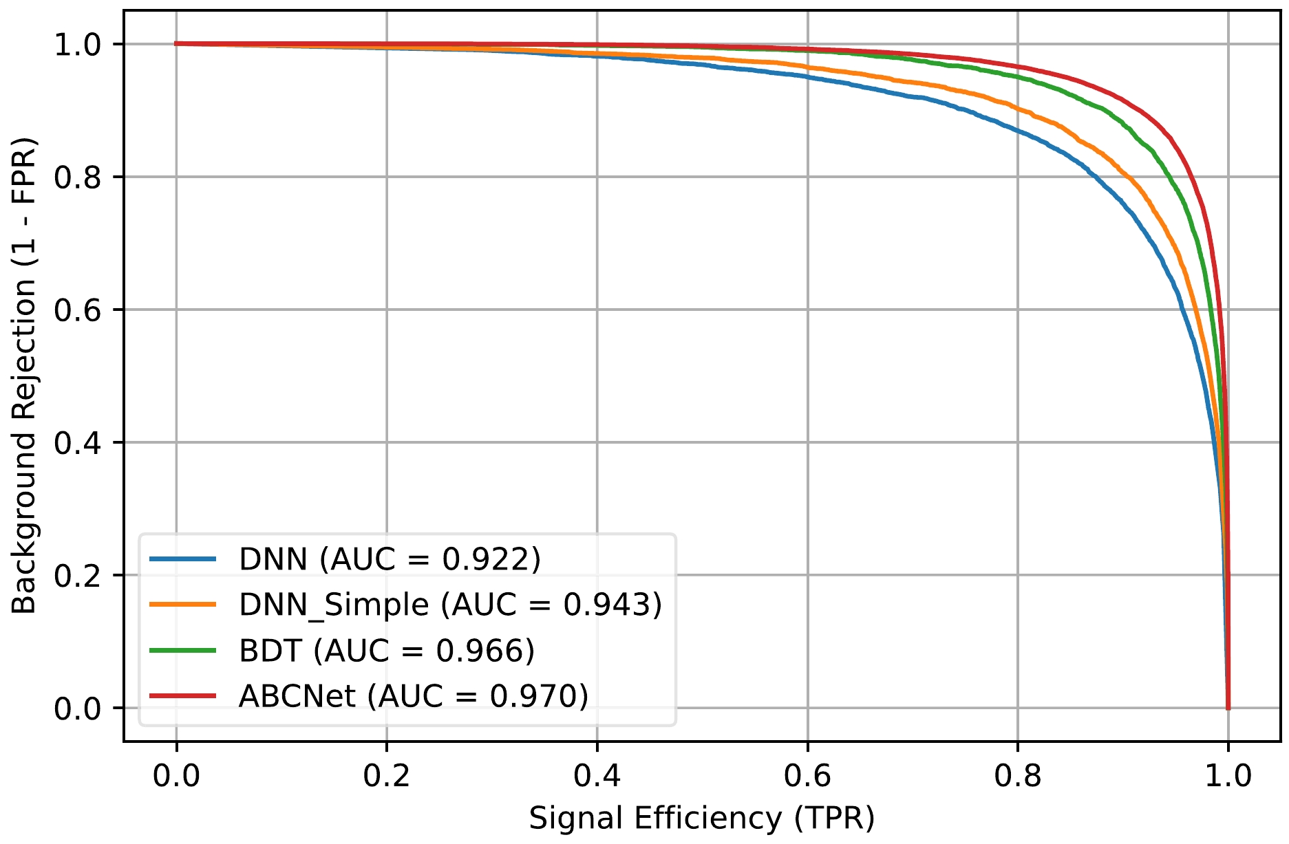
Figure 6. (color online) Comparison of background rejection versus signal efficiency for classification models: (a) BDT, (b) DNN with a single hidden layer, (c) DNN with more hidden layers, and (d) ABCNet.
Considering the AUC metric, ABCNet has the best performance compared to the BDT and DNNs using the same input, as shown in Fig. 6, as expected. A fully-connected DNN with many hidden layers performs even worse than the most reduced single-hidden-layer one.
We use the kinematic information of the τ, jet, and VLL candidates to predict the VLL mass, whose distribution is then used to derive the limits on each mass point. The predicted VLL mass distribution is a more involved mass reconstruction that uses the same DNN model as in Section 4.2 but changed from a classification to a regression task. The comparison between the predicted VLL mass and the VLL mass reconstructed using a simplified traditional method (see section 4) is shown in Fig. 7, where the former fits considerably better.
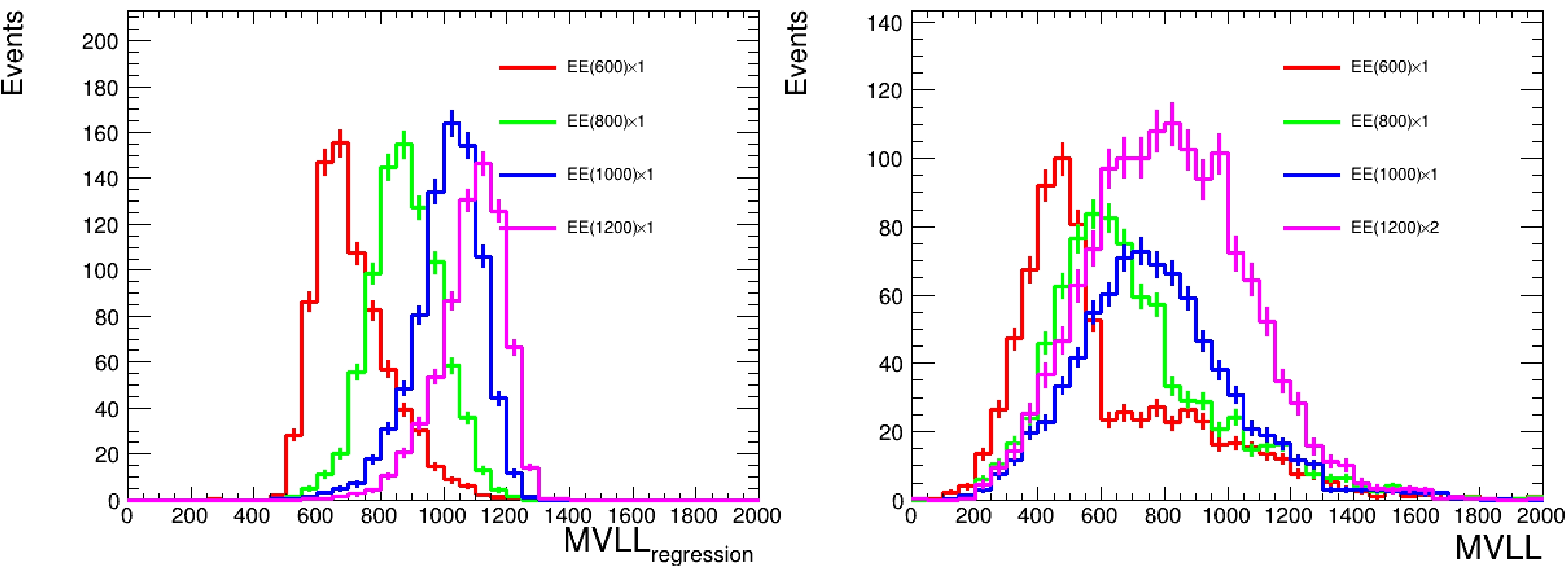
Figure 7. (color online) Comparison between the predicted VLL mass (left) and the simplified VLL mass reconstruction (right).
The signal region is defined as where the discriminant (that is, the ABCNet score) exceeds the threshold, which is chosen such that the best (that is, strongest) 95% confidence level (CL) upper limits are obtained for all VLL mass points. We search for peaks in the regressed VLL mass distributions by performing binned maximum likelihood fits using
${\tt{HistFactory}}$ [24] and${\tt{pyhf}}$ [25, 26]. Because observed yields are unavailable, "Asimov" data are used. We set the upper limit (UL) using the CL technique [27, 28]. Assuming the measurements performed are limited by the availability of data statistics, have well-constrained experimental systematics, and have excellent MC statistics, the background uncertainty is taken as the Poisson counting uncertainty for the expected background yield in each bin.Compared to the results of the analysis performed by the CMS experiment with the analyzed data corresponding to an integrated luminosity of 96.5
$ \mathrm{fb}^{-1} $ at a 13 TeV proton collider, the results at a 3 TeV muon collider are significantly improved. In the CMS experiment, an excess of 2.8 standard deviations over the SM background-only hypothesis was observed from the data at the representative VLL mass point of 600 GeV and no VLL masses were excluded at the 95% CL. In comparison, at the 3 TeV muon collider, VLL masses can be excluded at the 95% CL up to 1450 GeV with an integrated luminosity of only$ 0.01\ \mathrm{ab}^{-1} $ . The upper limit of the signal cross-section at the 95% CL corresponding to an integrated luminosity of$ 0.01\ \mathrm{ab}^{-1} $ is shown in Fig. 8.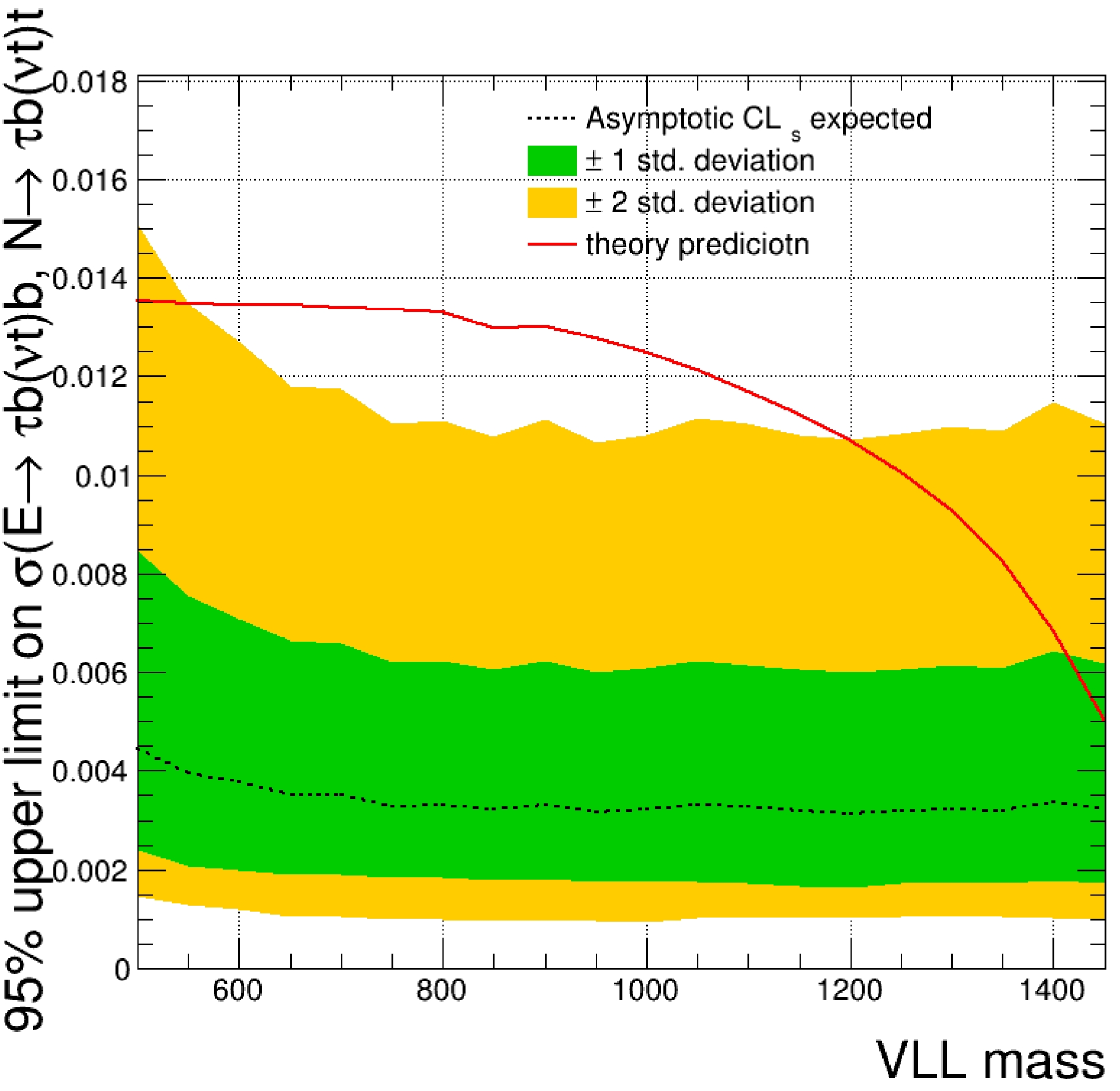
Figure 8. (color online) Expected 95% CL upper limits on the product of the VLL pair production cross section at a 3 TeV muon collider.
-
In this study, we investigate the potential for searching for VLLs at a future high-energy muon collider. The 4321 model, which is an ultraviolet-complete model and extends the SM gauge groups to a larger
${S U}(4) \times {S U}(3)' \times {S U}(2)_L \times {U}(1)'$ group, is considered in this study. In the model, a leptoquark is predicted as the primary source of lepton flavor nonuniversality, while the ultraviolet-completion predicts additional vector-like fermion families. In particular, VLLs are investigated via their couplings to SM fermions through leptoquark interactions, resulting in third-generation fermion signatures. Final states containing at least three b-tagged jets and two τ lepton multiplicities are considered. To improve the search sensitivity, BDT, DNN, and graph neural networks are trained to discriminate between signals and backgrounds. As a result, a 95% CL limit can be achieved for vector-like lepton masses up to 1450 GeV at a 3 TeV muon collider, with 1% of data corresponding to the target integrated luminosity. -
We thank Congqiao Li for illuminating and constructive discussions on neural network tuning and applications.
Vector-like lepton searches at a muon collider in the context of the 4321 model
- Received Date: 2023-05-19
- Available Online: 2023-10-15
Abstract: A feasibility study is performed on the search for vector-like leptons (VLLs) at a muon collider in the context of the "4321 model", an ultraviolet-complete model with rich collider phenomenology and the potential to explain several recent existing B physics measurements or anomalies. Pair production and decays of VLLs lead to an interesting final state topology with multi-jets and multi-tau leptons. In this study, we perform a Monte Carlo investigation with various machine learning techniques and examine the projected sensitivity on VLLs over a wide mass range at a TeV-scale muon collider. We find that a 3 TeV muon collider with only


 DownLoad: