


 Abstract
 HTML
HTML Reference
 Related
 PDF
PDF


-
In the recent years the cosmological theories have developed intensively due to various astrophysical probes [1, 2], adding new intriguing questions to modern physics. In the cosmological theories, one of the greatest challenges is related to the accelerated expansion of the known Universe [3, 4], an interesting phenomenon which is associated to the evolution of the Universe at the large scale structure [5−9]. Another key problem in cosmology is related to the dark matter phenomenon [10−12], having various ramifications at the level of galactic dynamics, being more local. All of these aspects suggest that we are far from understanding the nature and evolution of the Universe as a whole, leaving the door open for new theoretical directions and cosmological models [13]. From an astrophysical point of view, various observational studies can probe the nature and properties of the accelerated expansion [3, 14−19]. This phenomenon represents a curious aspect related to the fundamental ingredients of the Universe [20], having various ramifications in science and technology.
The simplest possible theoretical model related to the origin and characteristics of the accelerated expansion is the ΛCDM scenario [5], a proposal which cannot explain various fundamental aspects of this phenomenon [21]. To solve the dark energy problem, various theoretical ramifications have emerged [22]. In the modified gravity theories, the fundamental Einstein–Hilbert action is extended by adding specific invariants, which can be associated to the origin of the accelerated expansion [23−26]. One of the earliest models is the
$ f(R) $ scenario [27], a theoretical model grounded on the scalar curvature that naturally extends the Einstein–Hilbert action [28]. The modified gravity theories based on the$ f(R) $ invariant have been intensively examined in the past decades [28−33]. In different approaches, various alternative theories have been proposed [34−41], based on specific invariants in the corresponding action. For example, another origin of the dark energy phenomenon can be related to the$ f(G) $ models [42−44] based on the Gauss–Bonnet invariant. In these theories, one might consider the extension towards the interplay between the matter lagrangian and scalar curvature by applying a specific action$ f(R,L_m) $ [45, 46]. This particular model can be further generalized by considering a scenario based on$ f(R,T) $ [47], where T denotes the trace of the matter energy–momentum tensor [48]. In the latter theory, we can consider matter and geometry on equal footing, a specific interplay which can trigger the accelerated expansion [47]. All of these theories have been studied exhaustively in the recent years [49−57], showing specific advantages over the ΛCDM scenario [58]. The dark energy phenomenon can be also triggered by a scalar field embedded into action [5, 59], which can be minimally or non–minimally coupled [21] in the form of quintessence [60], phantom [61], or quintom scenarios [62−68]. In the modified gravity theories, a particular invariant based on the contraction between the matter energy–momentum tensor and Ricci tensor$ R_{\mu\nu}T^{\mu\nu} $ has been considered [51, 69]. Specifically, a possible interplay between the space–time geometry and fundamental characteristics of the matter component has been considered, which is embedded into the specific form of the energy–momentum tensor. Based on a theoretical perspective, this type of an approach is viable and can lead to different effects [70−79]. Hence, the extension towards an invariant based on the interplay between the Einstein tensor and energy–momentum tensor occurs naturally [80] and can lead to a viable modified gravity theory.In a recent study [80], the authors investigated the possible interplay between the Einstein tensor and matter energy–momentum tensor, embedding also specific derivative couplings. By considering a linear model in the proposed action, the perturbation analysis showed the viability of this type of a cosmological model. Considering the possible coupling between the matter energy– momentum tensor and Einstein tensor, we further extended the corresponding model by adding a general function, which depends on the interplay between the matter and geometry, embedded into the Lagrangian. To ensure a more general model, we also generalized the fundamental geometric part, embedding a specific component which further depends on the scalar curvature. Thus, the current model is broken down into a purely geometric segment reliant on the scalar curvature and another component. This second component, based on the interaction between matter and geometry, hinges on a new invariant that encapsulates the contraction of the energy-momentum tensor with the Einstein tensor.
The paper is organized as follows: in Sec. II, we briefly describe the cosmological model and corresponding field equations. Then, in Sec. III, by employing the dynamical system analysis, we investigate the generic model, which considers the curvature and matter couplings with the Einstein tensor. Furthermore, in Sec. IV, a specific subclass is investigated, where
$ f(R) $ part corresponds to the basic Einstein–Hilbert term. In Sec. V the last proposed model is investigated, where the matter– geometry function is represented by an exponential model. Lastly, in Sec. VI, we summarize the most important results and briefly present the concluding remarks. -
In this section, we briefly discuss the main elements corresponding to the present model, deducing the gravitational field equations in a cosmological context. In the subsequent discussion, we will introduce a model characterized by the following action:
$ \begin{equation} S=S_m+\int {\rm d}^4x \sqrt{-\tilde{g}} \big[f(R)+g(\phi) \big], \end{equation} $

(1) where a new generic function is added to the
$ f(R) $ part [32]. This function is further based on specific contractions between the Einstein tensor and energy–momentum tensor [80]:$ \begin{equation} \phi=G_{\mu \nu} T^{\mu \nu}. \end{equation} $

(2) This action can be regarded as a special case and complements the approach presented in Refs. [51, 69, 81]. Here, the energy–momentum tensor is defined in the usual manner as follows:
$ \begin{equation} T_{\mu \nu}=-\frac{2}{\sqrt{-\tilde{g}}}\frac{\delta(\sqrt{-\tilde{g}}L_m)}{\delta \tilde{g}^{\mu \nu}}, \end{equation} $

(3) where
$ L_m $ denotes the Lagrangian for the matter sector. Before proceeding to the derivation of the Einstein field equations, we introduce new elements for consideration. The trace of the energy–momentum tensor is defined as:$ T=T^{\mu \nu}\tilde{g}_{\mu \nu} $ . The variation of the energy–momentum tensor with respect to the inverse metric is equal to the following relation [80]:$ \begin{equation} \frac{\delta T_{\alpha \beta}}{\delta \tilde{g}^{\mu \nu}}=\frac{\delta \tilde{g}_{\alpha \beta}}{\delta \tilde{g}^{\mu \nu}}L_m+\frac{1}{2}\tilde{g}_{\alpha \beta}L_m \tilde{g}_{\mu \nu}-\frac{1}{2}\tilde{g}_{\alpha\beta}T_{\mu\nu}-2\frac{\partial^2 L_m}{\partial \tilde{g}^{\mu\nu} \partial \tilde{g}^{\alpha\beta}}. \end{equation} $

(4) Next, in our computations, we consider the following contraction [80]:
$ \begin{aligned}[b] \Sigma_{\mu\nu}=&G^{\alpha\beta}\frac{\delta T_{\alpha\beta}}{\delta \tilde{g}^{\mu\nu}}=-G_{\mu\nu}L_m+\frac{1}{2}G^{\alpha\beta}\tilde{g}_{\alpha\beta}(\tilde{g}_{\mu\nu}L_m-T_{\mu\nu}) \\&-2 G^{\alpha\beta}\frac{\delta^2 L_m}{\delta \tilde{g}^{\mu\nu} \delta \tilde{g}^{\alpha\beta}}. \end{aligned} $

(5) For the
$ f(R) $ part, the variation in the corresponding action with respect to the inverse metric leads to the associated energy momentum tensor [32],$ \begin{equation} T_{\mu\nu}^{f(R)}=\tilde{g}_{\mu\nu}f(R)-2 R_{\mu\nu}f_R+2\nabla_{\mu}\nabla_{\nu}f_R-2 \tilde{g}_{\mu\nu} \Box f_R, \end{equation} $

(6) where we introduced the derivative with respect to the scalar curvature,
$ f_R=\dfrac{\partial f(R)}{\partial R} $ . In the case of$ g(\phi) $ component, we obtained the following energy–momentum tensor [80]:$ \begin{aligned}[b] T_{\mu\nu}^{g(\phi)}=&\tilde{g}_{\mu\nu}g(\phi)+g_{,\phi}T R_{\mu\nu}-2 g_{,\phi} G_{\nu}^{\beta}T_{\mu\beta}-2 g_{,\phi} G_{\mu}^{\alpha}T_{\nu\alpha} \\&-g_{,\phi}R T_{\mu\nu}-\Box (g_{,\phi} T_{\mu\nu})+\nabla_{\alpha}\nabla_{\mu}(g_{,\phi}T_{\nu}^{\alpha})+\nabla_{\alpha}\nabla_{\nu}(g_{,\phi}T_{\mu}^{\alpha}) \\&-\tilde{g_{\mu\nu}}\nabla_{\alpha}\nabla_{\beta}(g_{,\phi} T^{\alpha\beta})+\tilde{g_{\mu\nu}}\Box(g_{,\phi}T)\\&-\nabla_{\mu}\nabla_{\nu}(g_{,\phi}T)-2g_{,\phi}\Sigma_{\mu\nu}, \end{aligned} $

(7) where
$ g_{,\phi} $ denotes the derivative with respect to the ϕ invariant, i.e.$ \begin{equation} g_{,\phi}=\frac{d g(\phi)}{d \phi}. \end{equation} $

(8) If we further apply the principle of least action, we obtain the final Einstein–like equation [32] as follows:
$ \begin{equation} T_{\mu\nu}^{f(R)}+T_{\mu\nu}^{g(\phi)}+T_{\mu\nu}^{m}=0. \end{equation} $

(9) This leads to the conservation relation as follows:
$ \begin{equation} \nabla^{\mu}\big[T_{\mu\nu}^{f(R)}+T_{\mu\nu}^{g(\phi)}+T_{\mu\nu}^{m}\big]=0. \end{equation} $

(10) This is also known as the continuity equation.
Next, we consider the following cosmological context associated to the FLRW model described by the metric:
$ \begin{equation} {\rm d}s^2=-{\rm d}t^2+a(t)^2\delta_{ij}{\rm d}x^i{\rm d}x^j, i,j=1,2,3. \end{equation} $

(11) In this instance, we consider a universal scale factor a that is dependent on cosmic time. Subsequently, we define the Hubble parameter in the conventional manner,
$ H=\dfrac{\dot{a}}{a} $ , where the dot denotes differentiation with respect to cosmic time. The energy–momentum tensor for the barotropic matter fluid is as follows:$ \begin{equation} T_{\mu\nu}=(\rho_m+p_m)u_{\mu}u_{\nu}+p_m g_{\mu\nu}, \end{equation} $

(12) where
$ \rho_m $ denotes the density and$ p_m $ denotes the pressure, connected via a barotropic equation of state of the form:$ p_m=w_m\rho_m $ . In the expression of the energy–momentum tensor, we embedded the 4-velocity$ u_{\mu}=\delta_\mu^0 $ . Furthermore, for the computations, we consider$ L_m=p_m $ . Subsequently, we will disregard the pressure in the matter sector, considering a theoretical framework that corresponds to a non-relativistic fluid without pressure. Within this cosmological setting, we derive the subsequent modified Friedmann relations [80]:$ \begin{equation} f(R)-6 f_R(\dot{H}+H^2)+6 H \dot{f_R}=\rho_m-g(\phi)-6 \rho_m g_{,\phi} \dot{H}, \end{equation} $

(13) $ \begin{equation} f(R)-2 f_R(\dot{H}+3 H^2)+2 \ddot{f_R}+4 H \dot{f_R}=-p_{\phi}, \end{equation} $

(14) $ \begin{aligned}[b] p_{\phi}=&g(\phi)-2 g_{,\phi}(\rho_m(3 H^2+\dot{H})+H \dot{\rho_m}) \\ &-6 H^2 \rho_m \big[2 \rho_m \dot{H}+H \dot{\rho_m} \big] g_{,\phi\phi}. \end{aligned} $

(15) Then, we can define the effective (total) equation of state as:
$ \begin{equation} w_{tot}=-1-\frac{2}{3}\frac{\dot{H}}{H^2}. \end{equation} $

(16) For the FLRW model without pressure, the matter–geometry invariant acquires the following value,
$ \phi=3 H^2 \rho_m $ , while the scalar curvature is equal to$ R=6(\dot{H}+2 H^2) $ . As expected, the resulting field equations reduce to the fundamental Einstein equations if$ g(\phi)=0 $ and$f(R)={R}/{2}$ . Similarly, the model describes$ f(R) $ theories of gravitation [32] in the absence of the interplay between the matter energy–momentum tensor and Einstein tensor. Finally, we note that at the linear level$ (g(\phi)=g_0\phi) $ , the equations reduce to the relations presented in Ref. [80]. As previously stated, the action presented in this study offers a generalization for the analysis presented in Ref. [80], extending the field equations in a generic manner. -
In this section, we discuss the physical features in the case where the coupling functions are as follows:
$ \begin{equation} f(R)=f_0 R^n, \end{equation} $

(17) and
$ \begin{equation} g(\phi)=g_0 \phi^m, \end{equation} $

(18) where
$ f_0, g_0, n, m $ are constant parameters. To study the cosmological model, we introduce the following dimensionless variables:$ \begin{equation} x=\dfrac{\dot{f_R}}{f_R H}, \end{equation} $

(19) $ \begin{equation} z=\frac{R}{6 H^2}, \end{equation} $

(20) $ \begin{equation} s=\frac{\rho_m}{6 f_R H^2}, \end{equation} $

(21) $ \begin{equation} u=\frac{g(\phi)}{6 f_R H^2}. \end{equation} $

(22) Furthermore, we use the next non–independent variables:
$ \begin{equation} \varsigma=\frac{\ddot{R}}{H^4}, \end{equation} $

(23) $ \begin{equation} \Delta=\frac{\dot{\rho_m}}{f(R) H}. \end{equation} $

(24) Considering the above definitions, we can rewrite the Friedmann constraint Eq. (13) in the following manner:
$ \begin{equation} z\left(\frac{1}{n}-1\right)+1+x=s-u-2 u m z +4 u m, \end{equation} $

(25) by reducing the dimension of the autonomous system with one unit. Hence, we remain with the following autonomous system
$ \{z,s,u\} $ . Considering the transformation to the e-folding number$N={\rm log}(a)$ , we can approximate the dynamics of the cosmological system at the linear level as follows:$ \begin{equation} \frac{{\rm d}z}{{\rm d}N}=z \left(\frac{x}{n-1}-2 z+4\right), \end{equation} $

(26) $ \begin{equation} \frac{{\rm d}s}{{\rm d}u}=\frac{\Delta z}{n}+s (-x)-2 s z+4 s, \end{equation} $

(27) $ \begin{equation} \frac{{\rm d}u}{{\rm d}N}=u \left(\frac{\Delta m z}{n s}+2 (m-1) (z-2)-x\right). \end{equation} $

(28) Then, the acceleration Eq. (14) can be expressed in the following manner:
$ \begin{equation} \Delta = \frac{s \left(6 n z \left((2 m (4 m-5)+3) (n-1) u+(n-2) x^2+2 (n-1) x-n+1\right)-6 (n-1) z^2 (2 m (2 m-1) n u+n-3)+n (n-1)^2 \varsigma\right)}{12 m^2 (n-1) u z^2}, \end{equation} $ 
(29) By obtaining a direct relation between Δ and ς, an additional relation between these two non–independent variables is obtained via direct differentiation of the Friedmann constraint Eq. (13), i.e.,
$ \begin{aligned}[b] & \frac{n (6 z ((n-2) x^2-n x+2 (n-1) (z-2)+x)+(n-1)^2 \varsigma)}{6 (n-1) z^2} \\=&\Delta +m u \Bigg(-\frac{2 n (z-2) (2 m (z-2)-2 z+1)}{z} \\&+\frac{\Delta (-2 m (z-2)-1)}{s}-\frac{2 n x}{n-1}\Bigg). \end{aligned} $

(30) In this approach, we can close the autonomous system of equations by obtaining specific relations for the non–independent variables ς and Δ. The final form of the autonomous system is as follows:
$ \begin{equation} \frac{{\rm d}z}{{\rm d}N}=-\frac{z \left(n u (2 m z-4 m+1)+2 n^2 z-4 n^2-n s-3 n z+5 n+z\right)}{(n-1) n}, \end{equation} $

(31) $ \begin{equation} \frac{{\rm d}s}{{\rm d}u}=s\left(2 m u z-4 m u+\frac{z}{n}-s+u-3 z+5+ \frac{A}{B}\right) , \end{equation} $

(32) $ \begin{aligned}[b] A=&n s (2 m u z-3 n+3)-2 m u (z^2 (2 m n u-(n-1) \\&\times(2 (m-1) n+1))+n z (6 m n-4 m u-6 m\\&-7 n+u+8)-(4 m-3) (n-1) n), \end{aligned} $

(33) $ \begin{equation} B=(n-1) n (m u (-2 m z+2 m-1)+s), \end{equation} $

(34) $ \begin{aligned}[b] \frac{{\rm d}u}{{\rm d}N}=&u\Bigg(2 m u z-4 m u+2 (m-1) (z-2)\\&+\frac{z}{n}-s+u-z+1+\frac{C}{D}\Bigg), \end{aligned} $

(35) $ \begin{aligned}[b] C=&m (n s (2 m u z-3 n+3)-2 m u (z^2 (2 m n u-(n-1)\\&\times (2 (m-1) n+1))+n z (6 m n-4 m u-6 m\\&-7 n+u+8)-(4 m-3) (n-1) n)), \end{aligned} $

(36) $ \begin{equation} D=(n-1) n (m u (-2 m z+2 m-1)+s). \end{equation} $

(37) The critical points for the autonomous system are obtained by setting the r.h.s. of Eqs. (26)–(28) to zero. In this case, we obtained the following critical points, associated to different cosmological solutions, which are attached to various epochs in the evolution of the Universe.
The first critical point investigated in our analysis is located in the phase space structure at the following coordinates:
$ \begin{equation} \mathcal{Q}_1=\big[z=0, s=2, u=0 \big], \end{equation} $

(38) By describing a radiation era
$ (w_{tot}=\dfrac{1}{3}) $ , where the dynamics in mainly influenced by the matter component via the s variable. The corresponding eigenvalues are as follows:$ \begin{equation} \Bigg[-2,3-7 m,\frac{4 n-3}{n-1} \Bigg]. \end{equation} $

(39) It can be observed that this epoch can be either stable or saddle, depending on the coupling parameters n and m.
The second critical point can be observed at the following coordinates:
$ \begin{equation} \mathcal{Q}_2=\Bigg[z=2-\frac{3}{2 n}, s=\frac{(13-8 n) n-3}{2 n^2}, u=0 \Bigg], \end{equation} $

(40) which is influenced by the value of the curvature coupling without any influence from the matter–geometry interplay. The total equation of state
$(w_{\rm tot}=\dfrac{1}{n}-1)$ can mimic an accelerated expansion era by fine–tuning the value of the curvature coupling parameter n. From a dynamical perpective, we obtained the following eigenvalues:$ \begin{aligned}[b] & \Bigg[3-\frac{3 m (n+1)}{n}, \\ &\frac{\pm \sqrt{256 n^4-864 n^3+1025 n^2-498 n+81}-3 n+3}{4 (n-1) n} \Bigg]. \end{aligned} $

(41) From a physical perspective, the value of the effective matter density parameter should be real and positive,
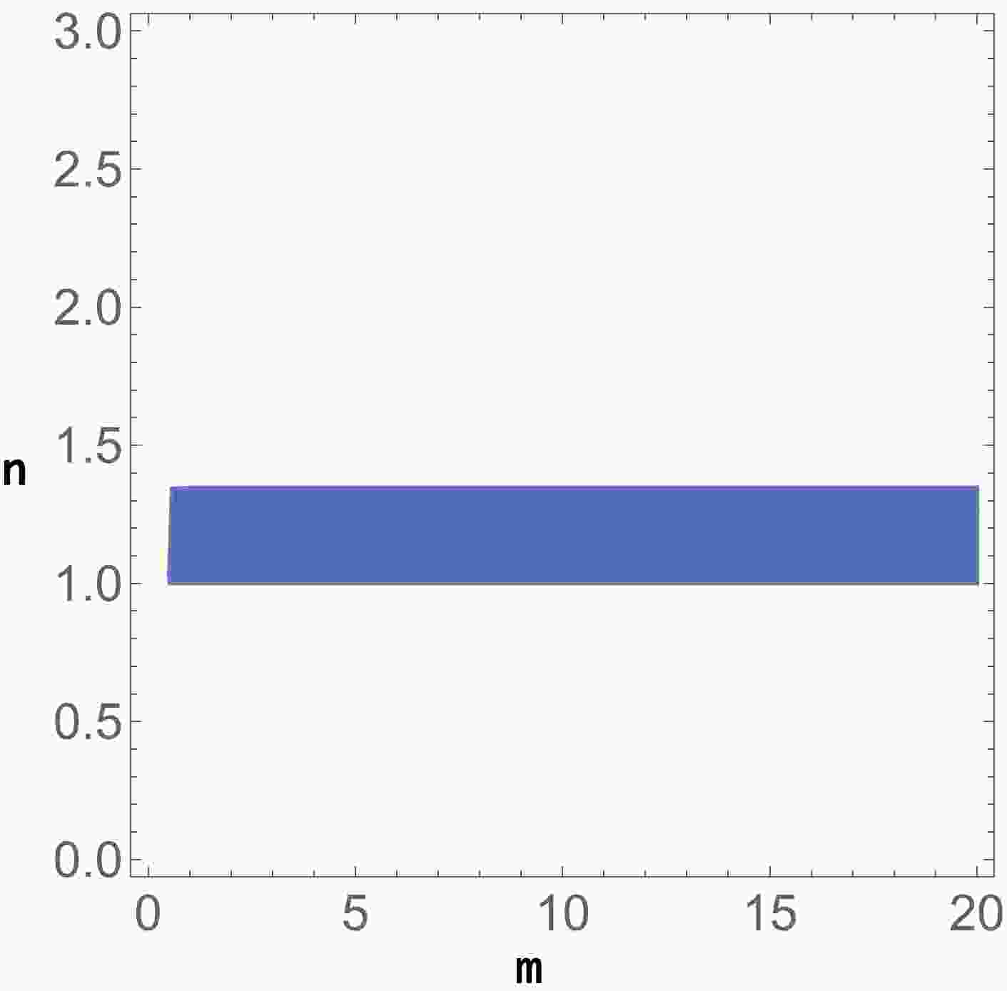
$ s>0 $ . We showed in Fig. 1, a specific region, where$ \mathcal{Q}_2 $ denotes a stable node, where all of the eigenvalues exhibit negative real parts, and the effective matter density parameter is restricted to$ [0, 1] $ interval. In Fig. 2, we observe that the value of the total equation of state depends on the scalar curvature coupling parameter. It should be noted that the main physical features for the critical points$ \mathcal{Q}_1 $ and$ \mathcal{Q}_2 $ are not influenced by the matter–geometry invariant. These solutions have been identified in different prior studies, being specific to the$ f(R) $ component in the action [21]. For these solutions, the matter–geometry invariant affects the physical features through the dynamics, influencing the values of the corresponding eigenvalues.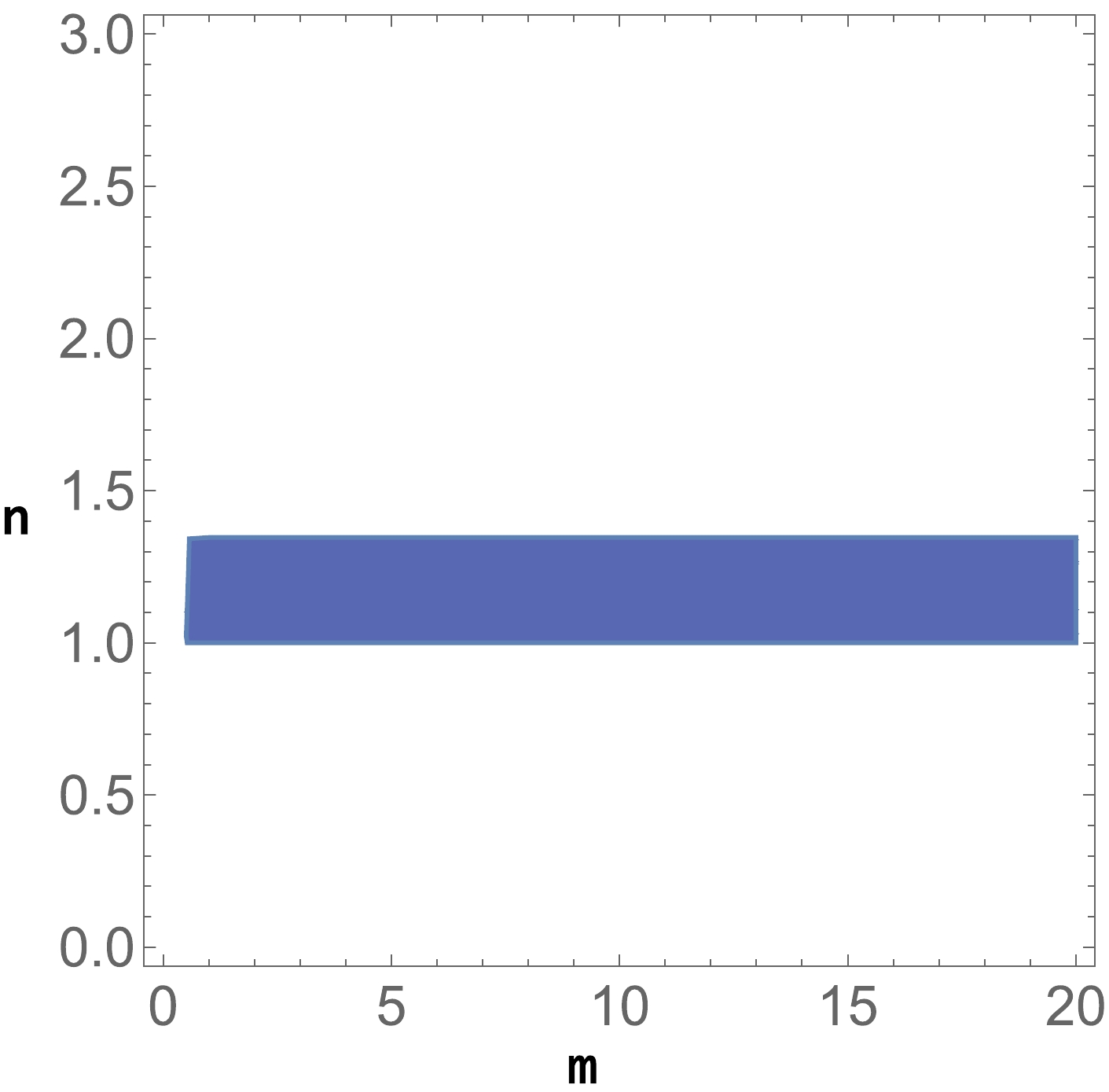
Figure 1. (color online) Specific region, where the critical point
$ \mathcal{Q}_2 $ , is stable and physically viable, with$ s \in [0, 1] $ .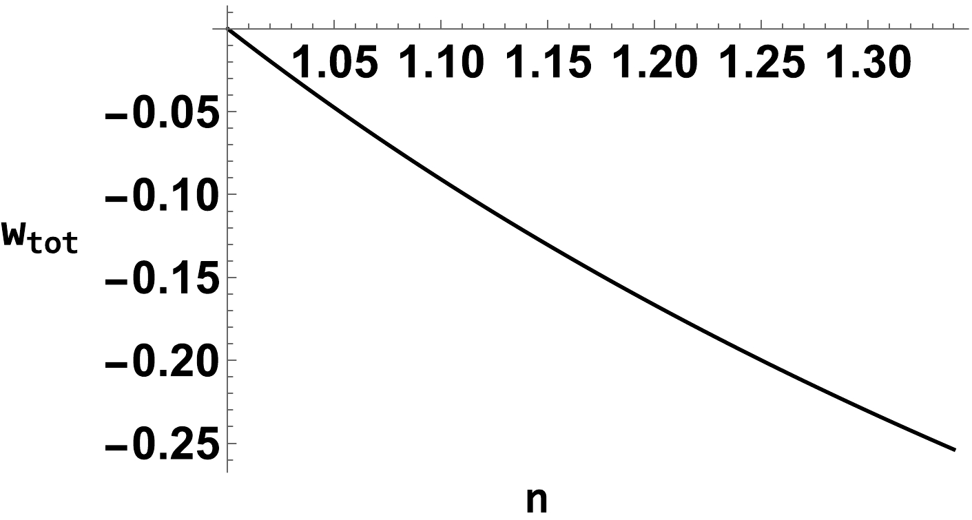
Figure 2. Variation in the total equation of state for the critical point
$ \mathcal{Q}_2 $ .The third critical point represents a geometrical dark energy solution with the dynamics driven mainly by the matter–geometry coupling invariant,
$ \mathcal{Q}_3=\Bigg[z=0, s=0, u=\frac{8 m-5}{8 m^2-6 m+1} \Bigg]. $

(42) The solution corresponds to a radiation epoch
$ (w_{\rm tot}=\dfrac{1}{3}) $ with the following eigenvalues:$ \Bigg[\frac{6-10 m}{1-2 m},\frac{5-8 m}{2 m-1},\frac{m (8 n-2)-4 n}{(2 m-1) (n-1)} \Bigg]. $

(43) By performing appropriate fine–tuning, we can obtain viable restrictions for the constant parameters such that this solution exhibits a saddle dynamic. For example, if we consider the following restriction,
$ \begin{equation} m<\frac{1}{2}\lor m>\frac{5}{8}, \end{equation} $

(44) then we can obtain a saddle behavior associated to the radiation era.
Next, solution
$ \mathcal{Q}_4 $ can be determined in the phase space structure at the following coordinates:$ \begin{aligned}[b] \mathcal{Q}_4=&\Bigg[z=0, s=-\frac{2 m (5 m-3) (9 m-5)}{(m-1) (m (18 m-13)+3)}, \\ u=&\frac{27 m-9}{m (18 m-13)+3}+\frac{2}{m-1} \Bigg], \end{aligned} $

(45) with a similar behavior as
$ \mathcal{Q}_3 (w_{\rm tot}=\dfrac{1}{3}) $ . In this case, the effective matter density parameter is affected by the matter–geometry interplay, without any influence by the curvature coupling. We obtained the following specific eigenvalues:$ \Bigg[-\frac{2 \left(35 m^2-36 m+9\right)}{14 m^2-23 m+9},\frac{5-9 m}{m-1},\frac{4 (m n+m-n)}{(m-1) (n-1)} \Bigg]. $

(46) Similar to the previous case, appropriate fine–tuning can identify specific regions where the behavior corresponds to a saddle dynamics, compatible to the known history of the Universe. In Fig. 3, we plot the variation in the matter density parameter for different values of m, the auxiliary variable associated with the interplay between matter and geometry.
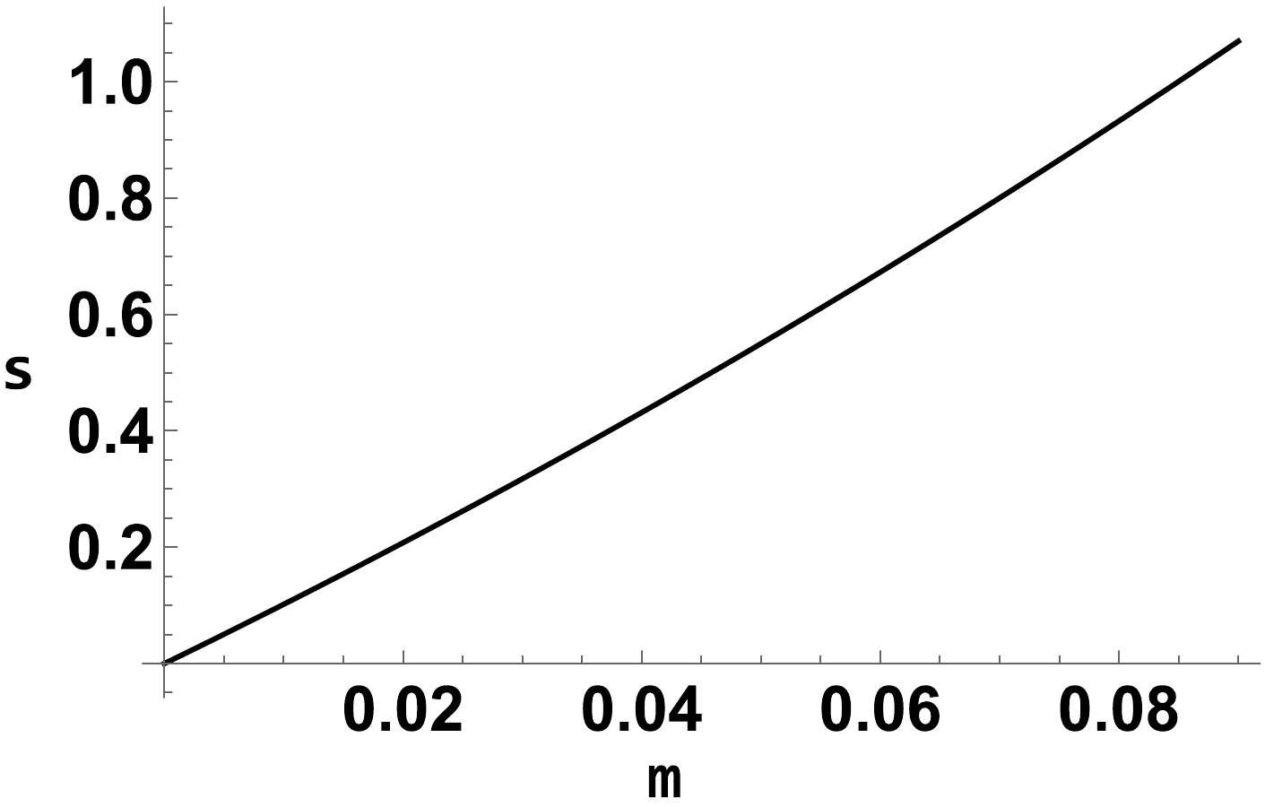
Figure 3. Variation in the s variable for the cosmological solution
$ \mathcal{Q}_4 $ .For the critical point
$ \mathcal{Q}_5 $ , we have the following coordinates:$ \mathcal{Q}_5=\Bigg[z=2, s=-\frac{2 m (n-2)}{(2 m-1) n},u=-\frac{2-n}{n-2 m n} \Bigg], $

(47) which is a particular solution corresponding to a de–Sitter epoch, where the dynamics corresponds to a cosmological constant,
$ (w_{\rm tot}=-1) $ . The equations related to the eigenvalues are too complex to present in this manuscript. As an alternative, we show in Fig. 4 a particular region of interest, where the cosmological solution is stable and physically viable, considering the following restriction:$ s \in [0, 1] $ . The numerical evolution toward$ \mathcal{Q}_5 $ solution is presented in Fig. 5, showing the compatibility between the analytical analysis and numerical approach$ (m=1, n=1.7) $ .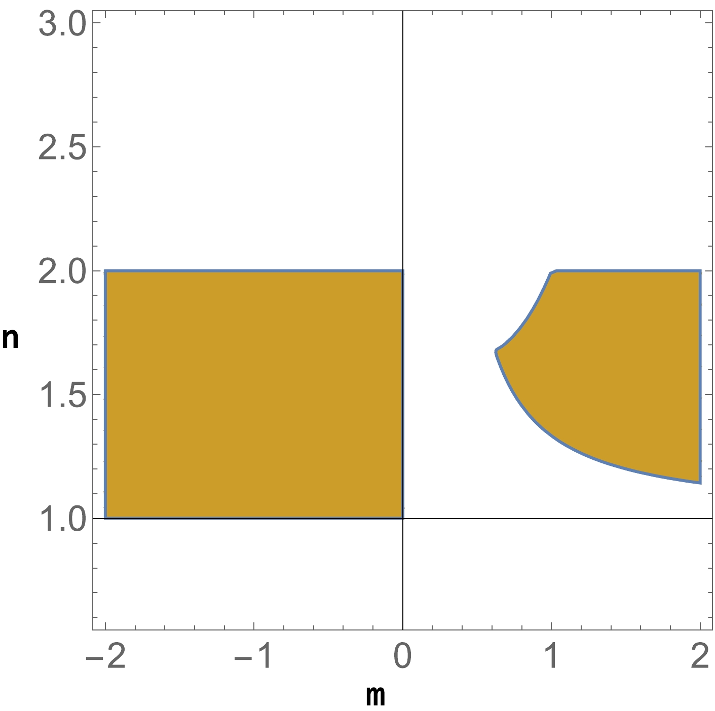
Figure 4. (color online) Region where the cosmological solution
$ \mathcal{Q}_5 $ is physically viable and stable$ s \in [0, 1] $ .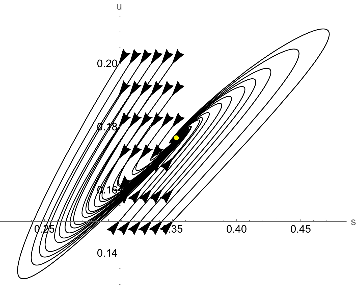
Figure 5. (color online) Evolution in the phase space toward the de–Sitter solution
$ \mathcal{Q}_5 $ for different initial conditions in the attractor basin.The last class of critical points can be determined at the following coordinates:
$ \begin{aligned}[b] \mathcal{Q}_6^{\pm}=&\Bigg[z=\frac{\pm\sqrt{4 m^2+4 (1-4 m) m n+(2 m n+n)^2}+m (6 n-2)-n}{4 m n}, s=0, \\u=&\frac{-28 m^2 n^2\mp\left(2 m (n-2)+2 n^2-3 n+1\right) \sqrt{4 m^2 ((n-4) n+1)+4 m n (n+1)+n^2}+\mathcal{R}}{8 m^2 n (3 m-n-1)} \Bigg], \end{aligned} $ 
(48) with
$ \mathcal{R}=40 m^2 n-4 m^2+4 m n^3-8 m n+2 m+2 n^3-3 n^2+n $ . Given that the two solutions are very similar, we discuss only the$ \mathcal{Q}_6^{+} $ case. As noted, the matter–geometry coupling and scalar curvature component influence the location in the phase space structure and corresponding dynamical features. This epoch can be considered as a curvature–matter–geometry solution, where the geometrical–matter components completely dominate in terms of effective density parameters. Based on this point, we obtained the following total equation of state:$ \begin{equation} w_{tot}=\frac{-\sqrt{4 m^2+4 (1-4 m) m n+(2 m n+n)^2}-4 m n+2 m+n}{6 m n}, \end{equation} $

(49) with influences from the scalar curvature coupling and matter–geometry invariant, respectively. By fine–tuning these parameters, we can obtain different classes of cosmological eras. For example, if we set
$ m=1 $ and$ n=\dfrac{2}{3} $ , then we can obtain a matter-dominated epoch, whereas for$ m=2 $ and$ n=\dfrac{1}{3} $ , we obtain a radiation behavior. In Fig. 6, we plot the variation in the total equation of state for different values of m and n parameters. We can observe that by fine–tuning we can obtain different values, corresponding to de–Sitter, quintessence, and phantom regimes. The final analytical expressions for the corresponding eigenvalues are very cumbersome and are not displayed in the manuscript. Instead, in Fig. 7 , we focus on displaying a non–exclusive possible interval, where the cosmological solution is represented by a saddle critical point.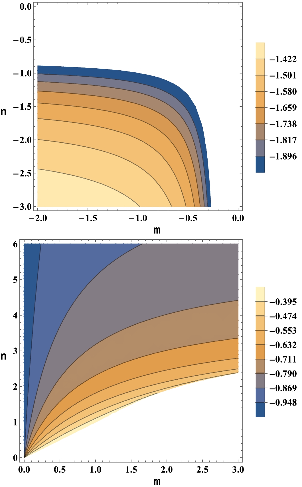
Figure 6. (color online) Variation in the total equation of state for
$ \mathcal{Q}_6^{+} $ curvature–matter–geometry solution.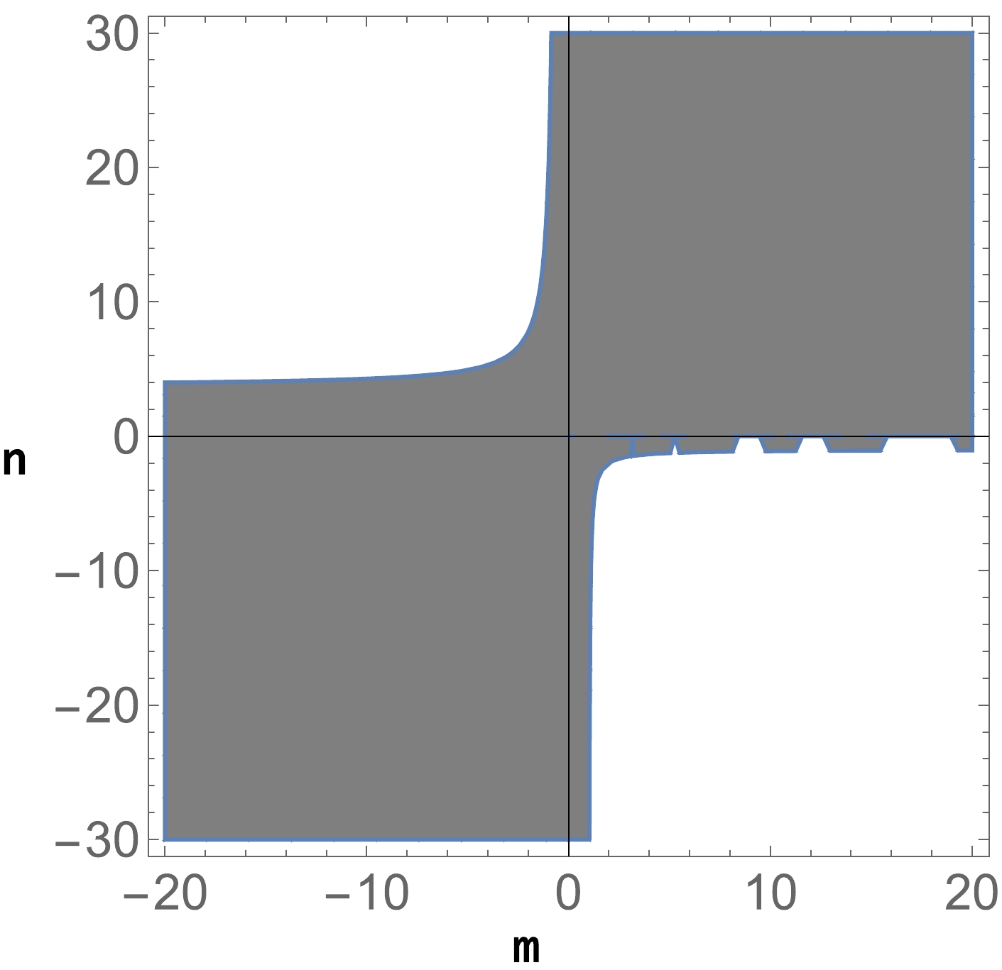
Figure 7. Region where the cosmological solution
$ \mathcal{Q}_6^{+} $ exhibits a saddle dynamical behavior. -
Next, we study the phase space structure for the case where the geometrical coupling function extends the fundamental Einsten–Hilbert action,
$ f(R,\phi)=\dfrac{R}{2}+g_0 \phi^{\alpha} $ , considering a power law representation for the matter–geometry invariant. In this case, we should introduce the following dimensionless variables:$ s=\frac{\rho_m}{3 H^2}, $

(50) $ x=\frac{g(\phi)}{3 H^2}, $

(51) $ y=\frac{\dot{H}}{H^2}. $

(52) In terms of dimensionless variables, the Friedmann constraint in Eq. (13) becomes:
$ \begin{equation} -1+s-x(2 \alpha y+1)=0, \end{equation} $

(53) which reduces the dimension of the phase space by one unit. Hence, the final independent dimensionless variables are:
$ \{s,x\} $ . Then, the associated dynamical equations have the following form:$ \begin{equation} \frac{{\rm d}s}{{\rm d}N}=-2 s y + \mathcal{L}, \end{equation} $

(54) $ \begin{equation} \frac{{\rm d}x}{{\rm d}N}=\frac{\alpha x \mathcal{L}}{s}+2 \alpha x y-2 x y, \end{equation} $

(55) where the additional non–independent variable is defined as:
$ \mathcal{L}=\dfrac{\dot{\rho_m}}{3 H^3} $ . The specific form of the acceleration equation (14) can be used to extract the non–independent variable,$ \begin{equation} \mathcal{L}=-\frac{s ((2 \alpha -1) x (2 \alpha y+3)-2 y-3)}{2 \alpha ^2 x}. \end{equation} $

(56) Hence, we obtain the final form of the autonomous system:
$ \begin{equation} \frac{{\rm d}s}{{\rm d}N}=\frac{s \left(x \left(4 \alpha ^2+2 \alpha +(1-4 \alpha ) \alpha s-1\right)+s-2 (\alpha -1) \alpha x^2-1\right)}{2 \alpha ^3 x^2}, \end{equation} $

(57) $ \begin{equation} \frac{{\rm d}x}{{\rm d}N}=\frac{-x (-4 \alpha +\alpha s+1)+s+2 \alpha (2-3 \alpha ) x^2-1}{2 \alpha ^2 x}. \end{equation} $

(58) As in the previous case, we identified the following critical points by analyzing the r.h.s. of the autonomous system.
The first critical point is located at the following coordinates:
$ \begin{equation} \mathcal{U}_1=\Bigg[s=\frac{2 \alpha }{2 \alpha -1}, x=\frac{1}{2 \alpha -1} \Bigg], \end{equation} $

(59) representing a de–Sitter epoch
$(w_{\rm tot}=-1)$ with the following eigenvalues:$ \begin{equation} \Bigg[\frac{2 \alpha (4-7 \alpha )\pm \sqrt{4 (\alpha -1) \alpha ((\alpha -7) \alpha +4)+1}-1}{4 \alpha ^2} \Bigg]. \end{equation} $

(60) For this point, we illustrate the value of s variable in Fig. 8, specifically for cases where α is negative. The s variable denotes the matter density parameter and, from a physical standpoint, should be positive. It is evident that this critical point corresponds to an era where the geometric coupling function is as a cosmological constant. When viewing it dynamically and in instances where α is negative, the point acts as an attractor with negative eigenvalues.
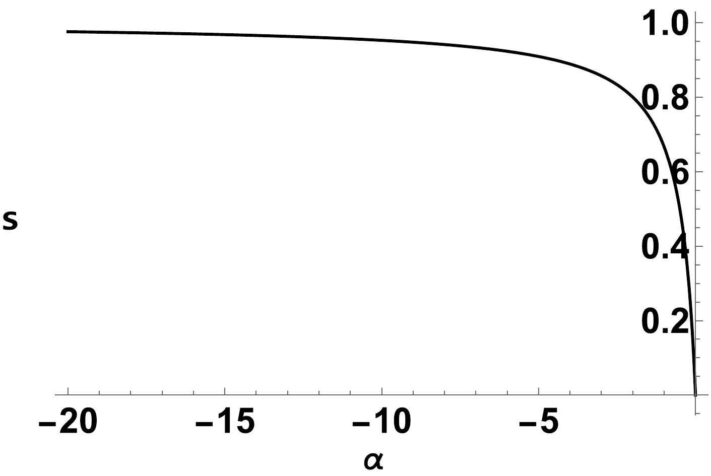
Figure 8. Value of the matter density parameter for the de–Sitter critical point
$ \mathcal{U}_1 $ .The second critical point represents an epoch located in the phase space at:
$ \begin{equation} \mathcal{U}_2^{\pm}=\Bigg[s=0, x=\frac{\pm \sqrt{-8 \alpha ^2+8 \alpha +1}-4 \alpha +1}{8 \alpha -12 \alpha ^2} \Bigg], \end{equation} $

(61) an epoch which can describe the accelerated expansion with the effective equation of state:
$ \begin{equation} w_{\rm tot}=\frac{-2 \alpha \pm \sqrt{1-8 (\alpha -1) \alpha }+1}{6 \alpha }, \end{equation} $

(62) which is sensitive to the value of the geometrical coupling parameter α. We note that the values of the matter density parameter is zero, a feature where the geometrical–matter coupling plays a fundamental role in the effective dynamics at the background level. Subsequently, we briefly describe
$ \mathcal{U}_2^{+} $ solution. The dynamics in a specific region for various values of the coupling parameter α is represented in Fig. 9. As shown, this critical point can explain various stages in the history of our Universe, the super–acceleration, radiation$ (\alpha =\dfrac{2}{3}) $ , and matter domination$ (\alpha =1) $ via fine–tuning. The accelerated expansion ($w_{\rm tot} < -\dfrac{1}{3}$ ) is obtained in the following interval:$ (\dfrac{1}{4} \left(2-\sqrt{6}\right)\leq \alpha <0) $ . Based on a dynamical perspective for the$ \mathcal{U}_2^{+} $ solution, we obtain the following eigenvalues:
Figure 9. Total equation of state for
$ \mathcal{U}_2^{+} $ critical point.$ \begin{aligned}\\[-10pt] \Bigg[ \frac{2 (3 \alpha - 2) \left(8 \alpha ^2 + 4 \left( \sqrt{-8 \alpha ^2 + 8 \alpha + 1} - 2\right) \alpha - \sqrt{-8 \alpha ^2 + 8 \alpha + 1} - 1\right)}{\alpha \left(\sqrt{-8 \alpha ^2+8 \alpha +1}-4 \alpha +1\right)^2}, \frac{2 (2 \alpha - 1) \left(24 \alpha ^3 - 6 \left( \sqrt{-8 \alpha ^2 + 8 \alpha + 1} + 3\right) \alpha ^2 + \sqrt{-8 \alpha ^2 + 8 \alpha + 1} + 4 \alpha + 1\right)}{\alpha ^2 \left(\sqrt{-8 \alpha ^2+8 \alpha +1}-4 \alpha +1\right)^2} \Bigg].\end{aligned} $ 
(63) Considering the analytical analysis of the previous eigenvalues,
$ \mathcal{U}_2^{+} $ solution is a stable node (with real and negative eigenvalues) in the following interval:$ \frac{1}{4} \left(2-\sqrt{6}\right)<\alpha <0 $ . Finally, we observe that the latter solution can explain a variety of cosmological eras, with a high sensitivity to the values of the geometrical–matter coupling embedded into the α coefficient. For the$ \mathcal{U}_2^{-} $ solution, we have a similar behavior. It should be noted that$ \mathcal{U}_2^{-} $ cannot explain matter and radiation epochs, while the accelerated expansion phenomenon is favored. -
In this section, we consider the following subclass of functions defined in the following manner:
$ \begin{equation} f(R,\phi)=\frac{R}{2}+g_0 {\rm e}^{\alpha \phi}, \end{equation} $

(64) where
$ f_0 $ and α denote constant parameters. As noted, the action is based on the fundamental Einstein–Hilbert action, extended with an exponential representation for the matter–geometry component. For this specific model, we introduce the following auxiliary variables:$ \begin{equation} s=\frac{\rho_m}{3 H^2}, \end{equation} $

(65) $ \begin{equation} x=\frac{g(\phi)}{3 H^2}, \end{equation} $

(66) $ \begin{equation} y=H^2 \dot{H}, \end{equation} $

(67) $ \begin{equation} z=\frac{1}{H^2}. \end{equation} $

(68) Moreover, we add the following non–independent variable:
$ \begin{equation} \mathcal{L}=H \dot{\rho_m}, \end{equation} $

(69) This can be used to form the autonomous system. In these variables, the Friedmann constraint Eq. (13) reduces to the following relation:
$ \begin{equation} 1+x+s(-1+18 \alpha x y)=0. \end{equation} $

(70) Then, the autonomous system becomes:
$ \begin{equation} \frac{{\rm d}s}{{\rm d}N}=\frac{z^2 \mathcal{L}}{3}-2 s y z^2, \end{equation} $

(71) $ \begin{equation} \frac{{\rm d}x}{{\rm d}N}=18 \alpha s x y-2 x y z^2+3 \alpha x \mathcal{L}, \end{equation} $

(72) $ \begin{equation} \frac{{\rm d}z}{{\rm d}N}=-2 y z^3, \end{equation} $

(73) while the acceleration Eq. (14) is equal to:
$ \begin{aligned}[b] &\frac{3 x \left(108 \alpha ^2 s^2 y+6 \alpha s \left(y z^2+3 \alpha \mathcal{L}+3\right)+z^2 (2 \alpha \mathcal{L}-1)\right)}{z^3}\\=&2 y z+\frac{3}{z} \end{aligned} $

(74) Given the specific form of the acceleration Eq. (14), we can extract the
$ \mathcal{L} $ variable, remaining with a three-dimensional dynamical system$ \{s,x,z\} $ . As in the previous cases, we determine the associated critical points by analyzing the right hand side of the autonomous system of differential equations. For the last physical model, where the coupling function is represented by an exponential, we identified only one class of cosmological solutions located in the phase space structure at the following coordinates:$ \begin{equation} \Xi_1=\Big[s=\frac{18 \alpha +z^2}{18 \alpha }, x=\frac{z^2}{18 \alpha } \Big]. \end{equation} $

(75) The critical line corresponds to a de–Sitter solution
$(w_{\rm tot}=-1)$ , describing an epoch where the dynamics induced by the interplay between geometry and matter mimics a cosmological constant behavior. In Fig. 10, we plot a specific region in the$ \{z, \alpha \} $ space, where the critical line$ \Xi_1 $ is viable considering the existence conditions.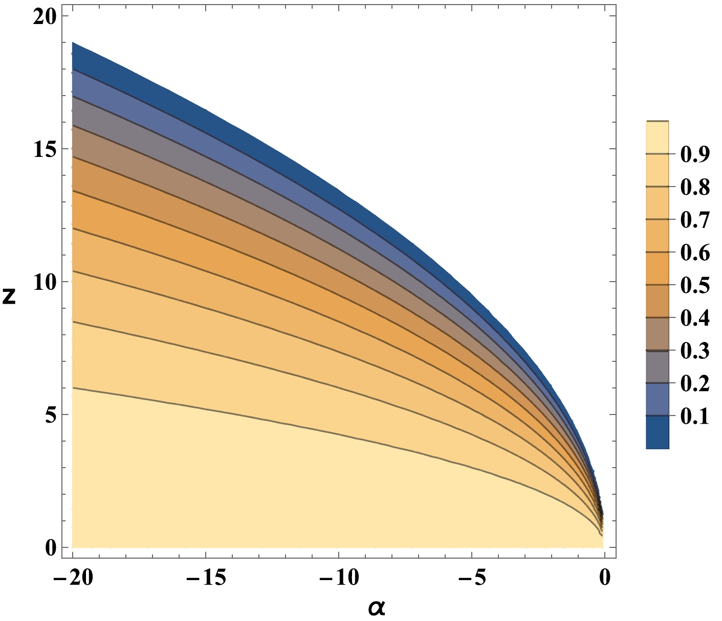
Figure 10. (color online) Specific region where the de–Sitter critical point
$ \Xi_1 $ is viable, with the matter density parameter in the$ [0, 1] $ interval.At this cosmological solution, we obtained the following eigenvalues,
$ \begin{equation} \Bigg[0,-\frac{2268 \alpha ^3+11 \alpha z^4+360 \alpha ^2 z^2 \pm \sqrt{\alpha ^2 \left(104976 \alpha ^4-23 z^8-720 \alpha z^6-7128 \alpha ^2 z^4-46656 \alpha ^3 z^2\right)}}{648 \alpha ^3+6 \alpha z^4+144 \alpha ^2 z^2} \Bigg], \end{equation} $ 
(76) describing a non–hyperbolic solution, which can saddle in some specific intervals. For example, if consider the following restrictions,
$ \begin{equation} z\in \mathbb{R}\land z\neq 0\land -\frac{z^2}{6}<\alpha <-\frac{z^2}{18}, \end{equation} $

(77) then we obtain a de–Siter epoch with a saddle behavior, where the dynamics corresponds to a cosmological constant added in the Einstein field equations.
-
In this study, we explored new cosmological models built on specific interactions between the matter energy–momentum tensor and geometric component, encapsulated within the Einstein tensor. Upon deriving the field equations where the matter aspect is portrayed by a barotropic fluid without pressure, we probed the physical characteristics of the corresponding dynamics using linear stability theory. This theory provides a distinct mathematical approach linked to global dynamics, pinpointing potential trajectories of our Universe within the phase space structure. Thus, in this study, we broadened the foundational Einstein–Hilbert action in a unique manner, contemplating a potential intertwining of matter and geometry. This is encapsulated in a pioneering invariant rooted in the contraction between the Einstein tensor and matter energy-momentum tensor. Our methodology amplifies previous research in modified gravity theories, as discussed in previous studies [51, 69, 80]. The first cosmological models [51, 69] in this direction proposed an action of the following type:
$ f(R,T,R_{\mu\nu}T^{\mu\nu}) $ , leading to interesting theoretical consequences. In Ref. [51], the authors examined several attributes of the de-Sitter solution and discussed matter instability within this framework. A comprehensive analysis addressing various cosmological issues can be found in Ref. [69], discussing the Dolgov– Kawasaki instability and specific cosmological applications related to the viability of this type of a proposal.Recently, in Ref. [80], the potential interaction between the Einstein tensor and matter energy-momentum tensor was explored at the linear level in the relevant action, using a perturbation approach. Furthermore, the authors delved into a nonminimal derivative coupling with the trace of the energy-momentum tensor, resulting in a feasible modified gravity theory. By considering this coupling between the matter energy-momentum tensor and Einstein tensor, we further refined the model, integrating a general function that reflects the relationship between matter and geometry within the Lagrangian. Utilizing linear stability theory, we examined the characteristics of the phase space structure, yielding distinct dynamical solutions that align with the recent evolutionary history of our Universe. The initial theoretical model we investigated is linked to a generic function of the following nature:
$ f(R,\phi)=f_0 R^n+g_0 \phi^m $ , with$ f_0, g_0, n, m $ constant parameters. In this case, the phase space is described by a three dimensional system, with various critical points, which correspond to various epochs aligned with the late-stage evolution of our Universe. For this model, we obtained the following classes of cosmological eras: de Sitter, radiation, and specific solutions, which depend on coupling parameters n and m. These solutions can describe the acceleration epoch and late–time dynamics in the Universe. For each class of cosmological solutions, we obtained possible constraints of the model parameters from a dynamical perspective, encoded into the specific values of the corresponding eigenvalues.The second cosmological model is associated with the following coupling function,
$ f(R,\phi)=\dfrac{R}{2}+g_0 \phi^{\alpha} $ , extending the fundamental Einstein–Hilbert action with a power–law model, which encodes non–minimal effects from the matter–geometry interplay. In the second case, the complexity of the phase space is diminished, correlating with a second-order dynamical system. The identified cosmological solutions can depict the de-Sitter epoch and late-time acceleration. Additionally, varying the coupling parameter yields diverse cosmological solutions, such as radiation or quintessence/phantom-like dynamics. Similar to the former situation, we derived potential dynamical constraints for each category of cosmological solutions.The last cosmological model is described by the following coupling function,
$f(R,\phi)=\dfrac{R}{2}+g_0 {\rm e}^{\alpha \phi}$ , with$ g_0, \alpha $ constant parameters. It is evident that this distinct cosmological system enhances the foundational Einstein–Hilbert term by incorporating a generic exponential function. This function captures specific contractions between the matter energy–momentum tensor and Einstein tensor. The related phase space is three-dimensional, boasting a single critical line tied to the de-Sitter epoch. This elucidates the late-time accelerated expansion in the Universe, a dynamic that mirrors that induced by a cosmological constant added to the Einstein–Hilbert term. Dynamically, this model can primarily account for the accelerated expansion and late-stage evolution. Therefore, in this particular model, early-time evolution can be addressed only through meticulous fine-tuning.It is apparent that this cosmological model, rooted in the interplay between matter and geometry, can account for various dynamic shifts in our Universe's evolution, making it a compelling avenue in modified gravity theories. This model offers further exploration potential through varied theoretical methodologies. For instance, we can embark on an observational study that might impose specific constraints on the distinct generic functions addressed in this study. Within such methodologies, specific reconstruction techniques can potentially be utilized, yielding varied physical outcomes during late-stage evolution. Each of these facets underscores both the potential and boundaries of our current cosmological approaches.
Physical aspects of ${ \boldsymbol{f}(\boldsymbol R,\boldsymbol G_{\boldsymbol\mu \boldsymbol\nu}\boldsymbol T^{\boldsymbol\mu \boldsymbol\nu})} $ modified gravity theories
- Received Date: 2023-04-07
- Available Online: 2023-10-15
Abstract: The paper extends basic Einstein–Hilbert action by incorporating an invariant derived from a specific contraction between the Einstein tensor and energy momentum tensor. This represents a non–minimal coupling between the space–time geometry and matter fields. The fundamental Einstein–Hilbert action is extended by considering a generic function


 DownLoad: