Prospects of gluino searches in multi-lepton channels in light of the ongoing LHC RUN-III

Supersymmetry (SUSY) [1−11] is the most promising beyond standard model (BSM) theory and resolves many of the lacunae of the standard model (SM) [12−28]. This elegant theory has been extensively studied over the last few decades both theoretically and experimentally and is currently being probed through various search channels in the ongoing Large Hadron Collider (LHC) experiment. Unfortunately, no appreciable deviation from SM predictions in the form of a statistically significant excess of events has been found. Therefore, the negative results from such searches during RUN-I [29−35] and RUN-II [36−50] of the LHC have imposed stringent bounds on the masses of sparticles (the supersymmetric counterparts of SM particles).

Owing to the large number of free parameters in SUSY models, particularly soft SUSY breaking parameters [51−53], it is challenging to interpret experimental results unless certain assumptions are made. For this reason, the ATLAS/CMS collaborations interpret their results in terms of simplified models in which certain sparticles of relevance are considered in the decay topology keeping others decoupled. These assumptions may not always be possible to realize within the context of the minimal supersymmetric standard model (MSSM). In this study, we consider the phenomenological MSSM (pMSSM), a reduced version of MSSM with 19 free parameters.

The strong sectors of SUSY, comprising gluinos and squarks, are the best probes to search for SUSY signals because of their large production rates. In RUN-II of the ATLAS experiment of the LHC, the gluino mass is excluded approximately up to 2.3 TeV in the channels involving $ jets+{{\not {E_T}}} $ [54], $ 1l+jets+{{\not {E_T}}} $ [55], and $ 2l+jets+ {{\not {E_T}}} $[56], assuming simplified models. In these analyses [54−56], all sparticles except for the gluino, lighter chargino (second lightest neutralino for Ref. [56]), and the lightest supersymmetric particle (LSP) (referred to here as the lightest neutralino) were assumed to be decoupled. The bound has almost been reached at the kinematic edge of the LHC. However, in Ref. [57], the authors discussed the effect of the inclusion of the second lightest neutralino ($ \tilde{\chi}_2^0 $) into the decay chain of gluinos along with the left and right squark mass hierarchy for the final state comprising $ jets+{{\not {E_T}}} $ and $ 1l+jets+{{\not {E_T}}} $. The inference of such a study is that it is possible to decrease the bound on gluino mass by an appreciable amount. Compressed SUSY scenarios are other examples in which such relaxation of bounds is possible [58−64].

The next step would be to observe the effects of the inclusion of heavier electroweakinos (in short, eweakinos) and sleptons/sneutrinos into the decay chain of the gluino, thereby lengthening the decay cascade even further. It must be noted that gluino searches have not been performed in more than two lepton final states. Therefore, the idea is to infuse more leptons in the final state arising from the decays of heavier eweakinos via the sleptons/ sneutrinos. This obviously will generate a more clean signal composed of multi-leptons in the LHC environment. Thus, the impetus of this study is to set the bounds on the gluino in the multi-lepton final states and explore the possibility of discovering it in the latest LHC RUN-III at a center-of-mass energy of 13.6 TeV .

It is worth mentioning that a study on direct production of heavier eweakinos was performed in [65] via a multi-lepton channel using LHC RUN-II data. Additionally, other phenomenological studies [66−70] probing eweakinos have been performed in light of ATLAS/CMS data [71−74]. In general, multi-lepton ¹ ($ nl+jets+{{\not {E_T}}} $) signals with $ n \ge 3 $ are the typical characteristic signatures of heavier eweakinos. The usual searches for gluinos apart from the multijet $ + {{\not {E_T}}} $ channel focus on the final state with up to $ 2l+jets+{{\not {E_T}}} $ at LHC RUN-II. However, if sleptons and heavier eweakinos are assumed to be lighter than the gluino, the following situations may arise:

● Lighter eweakinos and sleptons (that is, lighter than $ M_{\tilde{g}} $) would change the LHC RUN-II exclusion plot for gluinos. However, we do not intend to study this feature in this study.

● If heavier eweakinos appear in the decay cascade of gluinos and lighter eweakinos and sleptons constitute a compressed spectrum, the qualitative features of the signal change significantly. As a result, multi-lepton signals may become potential discovery channels for probing the strong sectors of the pMSSM through gluino searches [78−81]. The main objective of this study is to explore the potential of these multi-lepton channels in gluino searches at LHC RUN-III.

Bringing heavier eweakinos below the gluino mass has other theoretical motivations. The low higgsino mass parameter μ, which governs heavier eweakino masses, is believed to be favorable from the perspective of low fine tuning [82−87]. Introducing heavier eweakinos to gluino searches not only helps in collider searches but is also useful in explaining the WMAP/PLANCK [88, 89] measured relic density of dark matter (assuming the LSP, that is, the lightest neutralino ($ \tilde{\chi}_1^{0} $), emerges as a stable dark-matter candidate) and the precise measurement of the anomalous magnetic moment of the muon [90−93].

Many variants of the pMSSM are considered in this study, broadly categorized into two classes – wino type and higgsino type scenarios. Because the decays of gluinos to the electroweak sector depend on squark mixing, we vary the left (L) and right (R) squark compositions and make subcategories for them. For each type of model, two benchmark points (BPs) are chosen. The BPs considered in this study are consistent with the LHC RUN-II data from gluino searches in different final states. Owing to the presence of electroweakinos and sleptons in the decay cascades, the BPs chosen must also be consistent with their mass bounds obtained from LHC RUN-II. We also check that the BPs satisfy the WMAP/PLANCK data [88, 89] and the latest muon (g-2) data obtained from Fermilab [94].

In this study, we employ a multivariate analysis (MVA) technique for a better signal-to-background ratio. Such techniques are widely used in various collider analyses, such as particle identification, event reconstruction, and signal discrimination. MVA methods are used to classify particle interactions based on various kinematic input variables, called features. Some common MVA techniques used in collider physics are boosted decision trees (BDTs), neural networks (NNs), random forest (RF), and support vector machines (SVM). In this study, we use BDTs, which take a set of input features and split the input data iteratively based on these features.

The paper is organized as follows. In Sec. II, we construct and discuss the characteristic features of the models considered for our analysis. Sec. III covers the overall methodology adopted for this analysis. The constraints from LHC RUN-II data as well as muon (g-2) and the constraint on the relic density of dark matter from PLANCK data are also briefly described. The simulation strategy along with the selected BPs are also touched upon in this section. Sec. IV includes a comprehensive overview of gluino pair production along with its decay modes and a qualitative discussion on the yield of multi-lepton events with respect to our models. In Sec. V, the cut and count analysis (CCA) method for a particular signal topology and the details of the MVA method for all signals are presented. Additionally, the results obtained from the MVA method are discussed. Finally, we summarize our overall findings in Sec. VI.

We consider the pMSSM scenario in which the masses of the first two generations of squarks are greater than the mass of the gluino ($ m_{\tilde{q}} > m_{\tilde{g}} $). We study the pair production of gluinos in a proton-proton collision at a center-of-mass energy of 13.6 TeV at the LHC. The gluino mass is fixed by the SU(3) gaugino mass parameter $ M_3 $. The gluinos further decay into eweakinos along with a pair of light quarks ($ u,d,c,s $) via off-shell squarks. Obviously, the left(L)/ right(R) squark composition is important in determining the decays of the gluino. The following two cases might arise:

● The squark with a dominant SU(2) (that is, left) component takes the gluino to wino-type eweakinos with a pair of accompanying quarks.

● The squark with a dominant U(1) (that is, right) component facilitates the final state with a bino-type LSP with two quarks.

The electroweak sector in the R-parity conserving MSSM consists of a mixture of the spin-1/2 partners of the U(1) and SU(2) gauge bosons and Higgs bosons. The corresponding mass eigenstates are referred to as the charginos $ (\tilde{\chi}_j^{\pm}, j = 1, 2) $ and neutralinos $ (\tilde{\chi}_i^{0}, i = 1,2,3,4) $. The increasing order of indices conventionally implies increasing eweakino mass. The four parameters that determine the masses and compositions of these sparticles are $ M_1 $ (the U(1) gaugino mass parameter), $ M_2 $ (the SU(2) gaugino mass parameter), μ (the higgsino mass parameter), and $ \tan\beta $ (the ratio of the vacuum expectation values of the two neutral Higgs bosons). In this paper, we assume the parameter $ \tan\beta $ to be equal to 30. This choice is motivated by the fact that larger values of $ \tan\beta $ provide a better fit to the data on the parameter space allowed by the $ (g-2)_{\mu} $ constraint [66, 95, 96]. It also allows the mass of the SM-like Higgs boson to be as large as possible at the tree level. The lightest neutralino $ (\tilde{\chi}_1^{0}) $, which is the LSP, acts as a tenable dark matter candidate simply because it is stable and escapes detection at the LHC in the R-parity conserving SUSY scenario.

Sleptons are associated with either L- or R-type leptons, whereas sneutrinos are the superpartners of neutrinos. In this paper, it is assumed that all flavors of L(R)-type sleptons are degenerate in mass. Here, the masses of sneutrinos and the corresponding charged sleptons are non degenerate owing to the small contribution of the D-term. This always results in sneutrinos that are lighter than the charged sleptons and hence cannot produce leptons in their decay.

In this analysis, the Higgs sector does not play any role and is therefore kept decoupled, except for the Higgs boson of the SM, consistent with current experimental data.

Therefore, to summarize the interplay of various factors, we segregate our analysis into three scenarios:

1) Wino type model: The wino type model bears resemblance to the simplified models considered by the LHC collaboration. In the pMSSM, we specify the wino type model by setting $ M_1 < M_2 < \mu $. In this model, $ \tilde{\chi}_1^{\pm} $ and $ \tilde{\chi}_2^{0} $ (which are nearly mass degenerate) are predominantly composed of wino components, whereas $ \tilde{\chi}_1^{0} $ is bino like. On the other hand, the heavier eweakinos ($ \tilde{\chi}_2^{\pm} $, $ \tilde{\chi}_3^{0} $, and $ \tilde{\chi}_4^{0} $) are higgsino-like with masses governed by μ. To include the heavier eweakinos in the gluino decay chain, their masses must be smaller than that of the gluino. For these reasons, we must keep the value of μ smaller than $ M_3 $. We keep the slepton mass between those of $ \tilde{\chi}_1^{0} $ and $ \tilde{\chi}_1^{\pm}/\tilde{\chi}_2^{0} $ so that all the eweakinos can decay via sleptons, thereby increasing the size of the leptonic signals. We refer to this model as a light eweakino light slepton wino (LELSW) type model. In short, the hierarchy looks like

A pictorial representation of the mass hierarchy of relevant sparticles for this model is shown in Fig. 1.

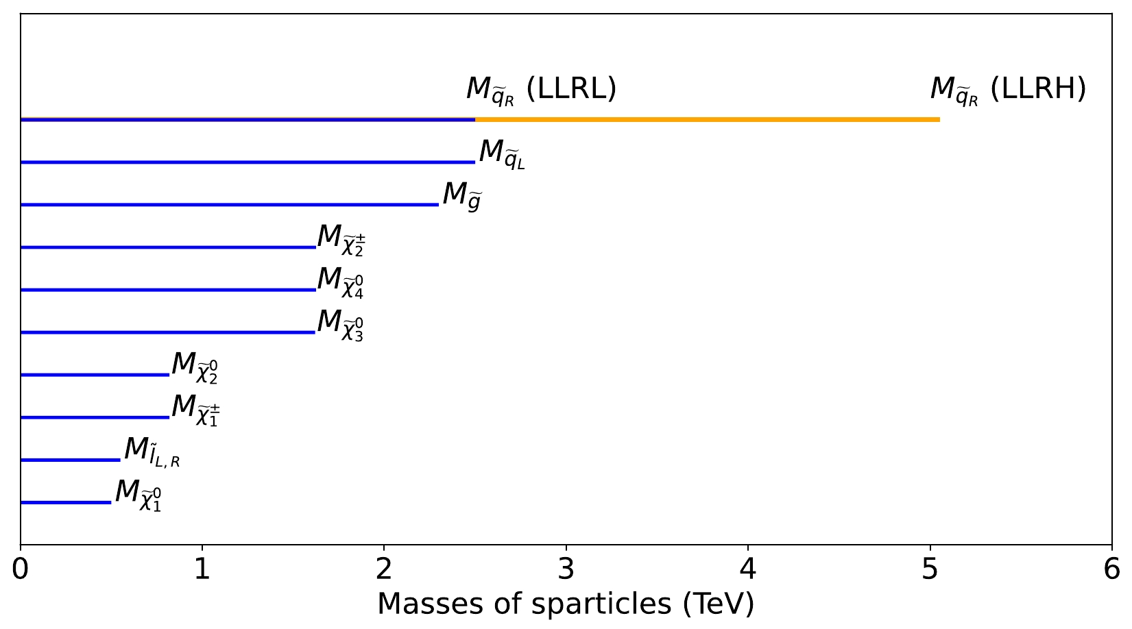
Figure 1.  (color online) Sparticle mass hierarchy and the values corresponding to BP1 for the light electroweakino light slepton wino (LELSW) models. The blue horizontal bars correspond to the scenario with left light and right light squark (LLRL). The orange horizontal bar corresponds to the left light and right heavy squark (LLRH) scenario in which all other mass parameters are the same as in the LLRL case.

2) Higgsino type models: In this type of model, we primarily focus on scenarios where $ \tilde{\chi}_1^{\pm} $, $ \tilde{\chi}_2^{0} $, and $ \tilde{\chi}_3^{0} $ contain large higgsino components and have closely spaced masses determined by μ, while the LSP is an admixture of bino and higgsino components. The mass hierarchy is determined by the gluino mass parameter $ M_3 $. To keep all the eweakinos lighter than the gluino, we must choose $ M_1, ~M_2,~\mu < M_3 $. Furthermore, the condition $ \mu \simeq M_1 $ is required to enhance the multi-lepton signatures with lepton multiplicities greater than 2. The two heavier eweakinos $ \tilde{\chi}_2^{\pm} $ and $ \tilde{\chi}_4^{0} $ are of the wino type. Their masses are approximately equal to $ M_2 $, with $ M_2 > \mu $. In this model, the slepton masses are kept between those of $ \tilde{\chi}_1^{0} $ and $ \tilde{\chi}_1^{\pm} $ so that all the eweakinos can decay into sleptons. We refer to these models as light eweakino light slepton higgsino (LELSH) type models.

In Fig. 2, we present the mass hierarchy of the relevant sparticles.

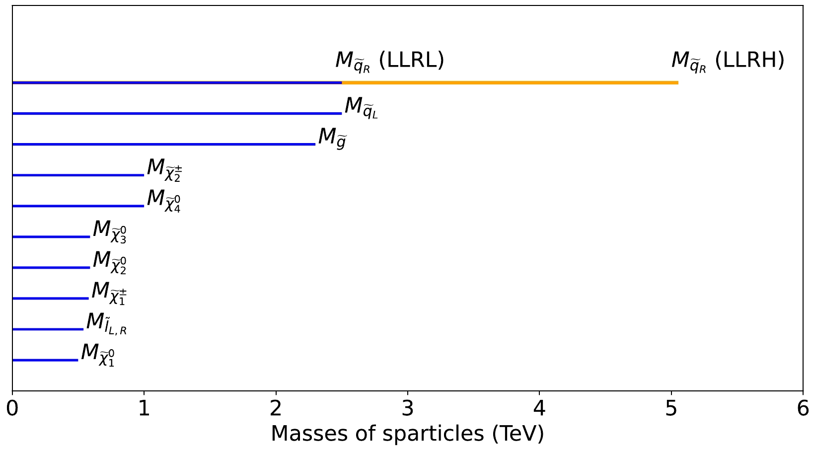
Figure 2.  (color online) Sparticle mass hierarchy and the values corresponding to BP1 for the light electroweakino light slepton higgsino (LELSH) models. The colors and conventions are the same as in Fig. 1.

3) Wino higgsino mixed type (Wiggsino) models: In the mixed type models, eweakinos (excluding the LSP) are combinations of higgsino and wino components and have closely spaced masses (that is, $ \mu \simeq M_2 $). In this scenario, the LSP is predominantly of the bino type, with its mass controlled by $ M_1 $. The sleptons are placed between the eweakinos and the LSP to obtain lepton-rich final states. The models are termed wino- higgsino mixed type (Wiggsino) models in our analysis. The mass hierarchy of the relevant sparticles is displayed in Fig. 3.

Figure 3.  (color online) Sparticle mass hierarchy and the values corresponding to BP1 for the wino higgsino mixed (Wiggsino) models. The colors and conventions are the same as in Fig. 1.

The above models are further subcategorized on the basis of the squark mass hierarchy, as mentioned at the beginning of this section. The squarks contribute to gluino production via the t/u-channel diagrams. Most importantly, because the squarks are heavier than the gluinos in our analyses, the gluino decays into various eweakinos are dictated by off-shell squark propagation. Thus, the following two major scenarios appear:

● In the left light right light squark (LLRL) mass models, both L- and R-squarks have similar masses just above the gluino mass, that is, ($ M_{\tilde{g}} < M_{\tilde{q}_{L,R}} \simeq 2.5 $ TeV).

● In the left light right heavy squark (LLRH) mass models, the L-squarks are light and positioned just above the gluino mass in the mass scale ($ M_{\tilde{q}_{L}} \simeq 2.5 $ TeV). However, the R-squarks are made considerably heavier, $ M_{\tilde{q}_{R}} > 5 $ TeV, and are hence decoupled.

If the L-squark is decoupled, regardless of the mass of the R-squark, the gluino most likely decays into $ q \bar{q} \tilde{\chi}_1^{0} $, giving multijet final states and making this an uninteresting case for this study.

In this section, we first discuss various constraints on the pMSSM parameters that are the guiding principles in selecting the BPs of various models considered in this study. Next, we describe two chosen BPs. Finally, we give an outline of the simulation techniques used in this study, particularly emphasizing the MVA method.

SUSY has been investigated for a long time. Hence, most of the avenues are constrained by experimental data. In this section, we briefly mention the various relevant constraints from the LHC and other low energy experiments. We abide by these bounds when selecting the BPs.

The ATLAS collaboration has explored several search channels to constrain the masses of the gluino and squarks. In RUN-II, the limits on the mass of the gluino (squark) for an integrated luminosity of 139 $\rm fb^{-1}$ for various final states are almost at the edge of the kinematic reach of the LHC. The constraints on the gluino (squark) mass for negligible LSP mass are summarized in Table 1.

Pair production	Signal topology	Bounds on gluino (squarks) for negligible mass of the LSP /GeV	Ref.
$ \tilde{g} $ ($ \tilde{q} $)	$ jets+{{\not {E_T}}} $	2300 (1850)	[54]
$ \tilde{g} $ ($ \tilde{q} $)	$ 1l+jets+{{\not {E_T}}} $	2200 (1400)	[55]
$ \tilde{g} $ ($ \tilde{q} $)	$ 2l+jets+{{\not {E_T}}} $	2250 (1550)	[56]

Table 1.  Bounds on gluino (squark) masses from various search channels at LHC RUN-II.

Note from Fig. 13(14) of Ref. [54] that there is practically no bound on the mass of $ \tilde{g} $ ($ \tilde{q} $) for $ M_{\tilde{\chi}_1^0} \gtrsim $ 1.1 (0.8) TeV for $ jets +{{\not {E_T}}} $. We can further infer from Fig. 8 of Ref. [55] that the bound on the mass of $ \tilde{g} $ ($ \tilde{q} $) for $ M_{\tilde{\chi}_1^0} \gtrsim $ 1.26 (0.7) TeV does not exist in the final state comprising $ 1l+jets+{{\not {E_T}}} $. A similar observation holds for $ M_{\tilde{\chi}_1^0} \gtrsim $ 1.4 (0.9) TeV in the $ 2l+jets+{{\not {E_T}}} $ final state, which can be seen in Fig. 16 of Ref. [56]. More details can be found in the given references.

Figure 13.  (color online) ROC curve corresponding to the model mentioned in Fig. 11 for the signal state comprising $ 3l+jets+{{\not {E_T}}} $.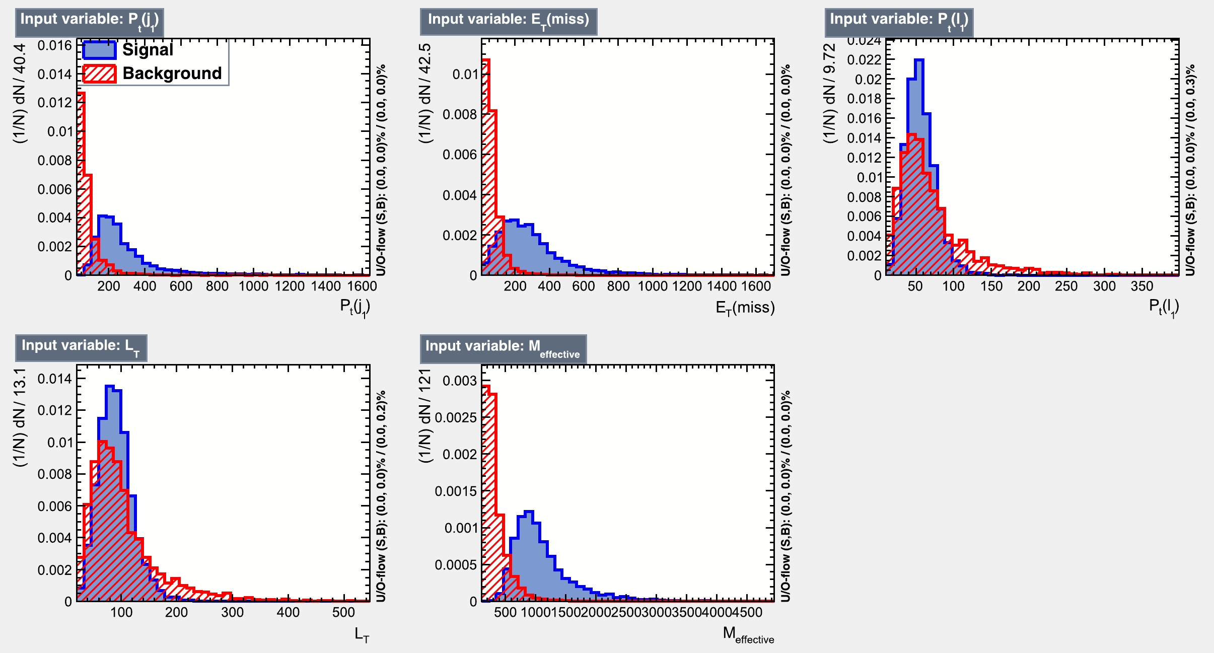

Figure 8.  (color online) Signal (blue) and background (red) distributions of the input features in the final state comprising $ 2l+jets+{{\not {E_T}}} $ with the same sign same flavor (SSSF) lepton pair corresponding to BP2 of the same model mentioned in Fig. 5.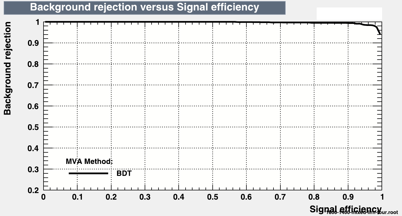

Figure 16.  (color online) ROC curve corresponding to the model mentioned in Fig. 14 for the signal state comprising $ 4l+jets+{{\not {E_T}}} $.

During LHC RUN-II, the ATLAS collaboration conducted searches for SUSY through electroweak sparticle pair production. The searches were performed in different multi-lepton channels, such as $2l+{\not {E}_T}$ [97] for lighter eweakinos ($ \tilde{\chi}_1^+ $, $ \tilde{\chi}_1^- $) and sleptons and $ 3l+{{\not {E_T}}} $ [98] for lighter eweakinos ($ \tilde{\chi}_1^{\pm} $, $ \tilde{\chi}_2^0 $). The results have been interpreted in terms of simplified models. At an integrated luminosity of 139 fb$ ^{-1} $, no significant excess of signal events over SM backgrounds have been observed. The exclusion limits for the masses of eweakinos and sleptons are summarized in Table 2.

Pair production	Signal topology	Bounds on gluino (squarks) for negligible mass of the LSP /GeV	Ref.
$\tilde{\chi}_1^\pm \tilde{\chi}_1^{\mp}$	$ 2l+{{\not {E_T}}} $	1000	[97]
$ \tilde{l} \tilde{l}^{*} $	$ 2l+{{\not {E_T}}} $	700	[97]
$\tilde{\chi}_1^\pm \tilde{\chi}_2^{0}$	$ 3l+{{\not {E_T}}} $	640	[98]

Table 2.  Bounds on eweakinos and sleptons from various search channels at LHC RUN-II.

From Fig. 7(c) in [97], we can infer that the bound on the mass of sleptons evaporates if $ M_{\tilde{\chi}_1^0} \gtrsim 420 $ GeV in the $ 2l+{{\not {E_T}}} $ final state. Furthermore, from Fig. 7(b) of Ref. [97], we observe that if $ M_{\tilde{\chi}_1^0} \gtrsim 500 $ GeV, there is no constraint on $ M_{\tilde{\chi}_1^{\pm}} $ in the decay topology where $ \tilde{\chi}_1^{\pm} $ decays via sleptons. It is also clear from Fig. 16 that the ATLAS collaboration [98] does not provide a lower bound on the mass of the lighter eweakinos for $ M_{\tilde{\chi}_1^0} $ beyond 300 GeV in the $ 3l+{{\not {E_T}}} $ final state. More information about the search of eweakinos/sleptons can be found in the given references.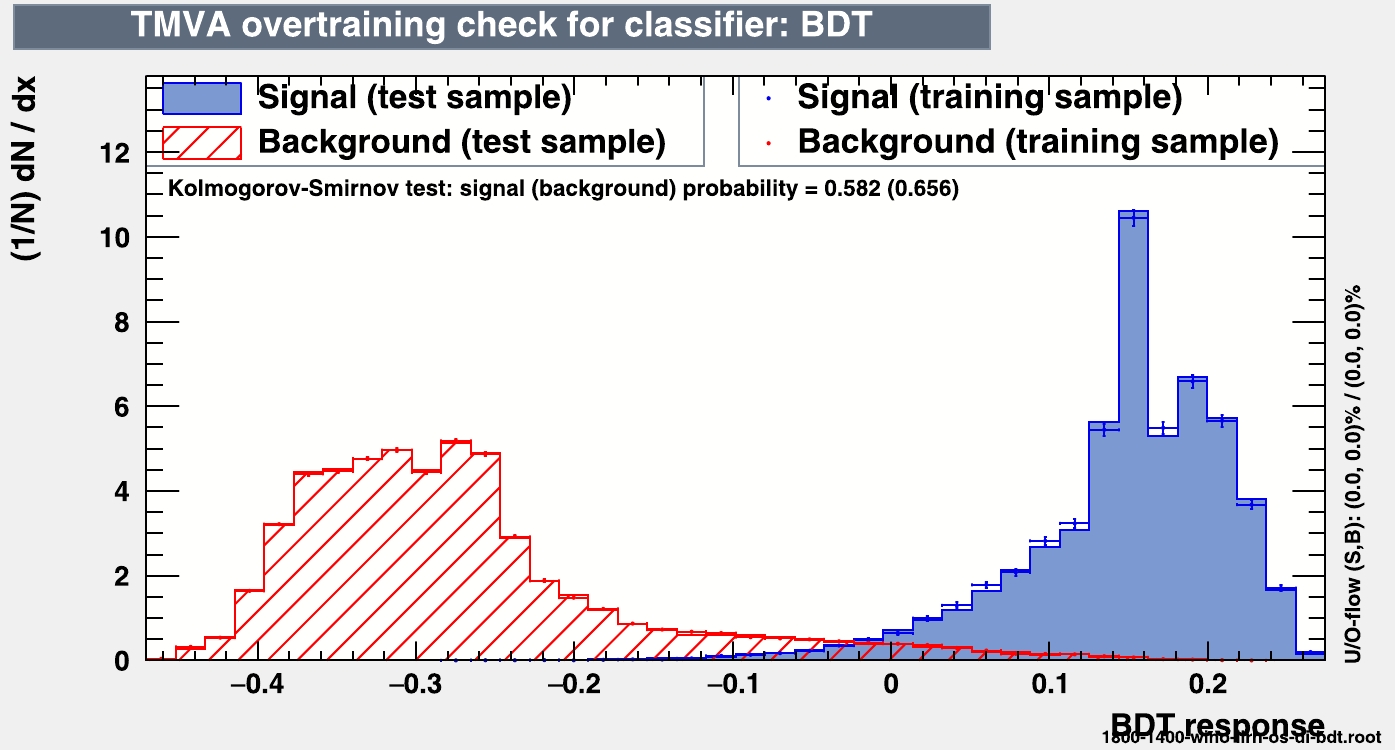

Figure 7.  (color online) For the purpose of illustration, we present the over-training check of the BDT response for the model mentioned in Fig. 5 using the parameter set of BP2.

● The SUSY mass spectra for the BPs must satisfy the SM-like Higgs boson mass constraints, that is, $ 122 < M_h < 128 $ GeV, with the central value of 125 GeV [99, 100]. This can be obtained using an appropriate choice of the trilinear soft breaking term for the top squark ($ A_t $) and CP-odd Higgs mass ($ M_A $). The theoretical uncertainty [101, 102] in determining the Higgs mass in a typical SUSY scenario is dealt with by allowing a mass window of $ \pm 3 $ GeV.

● Tantalizing hints of new physics arise from the long standing discrepancy between experimental data and the SM prediction of the anomalous magnetic moment of muons, denoted by $a_{\mu}={2}(g-2)_{\mu}/2$. The SUSY contribution denoted as $a^{\rm SUSY}_{\mu}$ becomes significant if the masses of charginos, neutralinos, and smuons are relatively light. It also depends on $ \tan\beta $, the ratio of the vacuum expectation values of the two Higgs doublets. Therefore, we can constrain the SUSY parameter space by comparing the measured values of $ \Delta a_{\mu} $, which is the difference between the experimental value of $ a_{\mu} $ and the SM prediction. According to the results of the Fermilab National Accelerator Laboratory (FNAL), the value of $ \Delta a_{\mu} $ along with the uncertainty is given by [94]

● In this analysis, we also consider the constraint on the dark matter relic density estimated by the WMAP/PLANCK data [89] with a small observational uncertainty:

where $ h=0.733\pm 0.181 $ [103] is the Hubble constant in units of 100 km/Mpc-s.

To analyze our models and assess the potential for discovery, we choose two BPs corresponding to each model described in Sec. II. One is selected from the edge of the gluino exclusion region, whereas the other is taken from the compressed region where the gluino and LSP are similar in terms of mass.

BP1 corresponds to the heavier mass of the gluino resulting in a smaller production cross-section, whereas BP2 corresponds to the reverse situation. BP1 offers more kinematic phase space for the reconstructed objects, whereas the same becomes more limited in the case of BP2. Moreover, the BPs are chosen in such a way that they can pass the collider constraints mentioned in Sec. III.A. It is evident from Sec. III.A that if the mass of the LSP is set to be above 500 GeV, the BPs satisfy the mass bounds obtained from the electroweak searches at LHC RUN-II.

Except for a few models, the BPs corresponding to all models satisfy other constraints, such as the PLANCK data for dark matter relic density and the precise value of the anomalous magnetic moment of muons, within the feasible allowed range of uncertainty. The BPs are chosen so that the estimated value of $ \Delta a_{\mu} $ (which is assumed to be the SUSY contribution) is considered to lie within $ 4\sigma $ of the central value.

For the choice of the BPs, it is assumed that third generation squarks are decoupled and all other soft-breaking trilinear terms are set to be zero, except for the trilinear soft breaking term for the top quark, $ A_t $, which is set to be 5 TeV to obtain an SM-like Higgs mass of approximately $ M_h=125 $ GeV. Throughout the study, $ \tan\beta $ is set as 30, and the value of the pseudo scalar Higgs mass $ M_A $ is taken to be around 3 TeV. The choice of $ M_A $ is not crucial for the collider analysis but will have substantial significance in satisfying the PLANCK constraints through H-resonance or CP-odd Higgs A-resonance annihilations (for more details, see Ref. [57]). This particular value of $ M_A $ is chosen for illustration purposes and does not affect the generality of the study. All other mass parameters along with the relic density, $ \Delta a_{\mu} $, and cross-section values are presented in Table 3.

BP	Model	$M_{\tilde{g}}$ /GeV	$M_{\tilde{\chi}_1^0}$ /GeV	$M_{\tilde{\chi}_1^\pm}$ /GeV	$M_{\tilde{\chi}_2^0}$ /GeV	$M_{\tilde{\chi}_3^0}$ /GeV	$M_{\tilde{\chi}_4^0}$ /GeV	$M_{\tilde{\chi}_2^\pm}$ /GeV	$M_{\tilde{l}^\pm}$ /GeV	$\Omega_\chi h^2$	$\Delta a_\mu \times 10^{-11}$	Production cross-section/fb
												LLRL	LLRH
BP1	LELSW	2300	500	820	820	1621	1624	1624	550	0.021	73.4	0.153	0.184
	Wiggsino	2300	500	800	800	879	920	919	550	0.126	77.4
	LELSH	2300	500	580	589	591	1000	1000	540	0.325	79.0
BP2	LELSW	1800	1400	1455	1455	1770	1783	1779	1430	0.589	15.9	2.15	2.56
	Wiggsino	1800	1400	1550	1552	1630	1672	1670	1450	0.112	15.7
	LELSH	1800	1400	1460	1475	1476	1700	1700	1430	0.254	15.9

Table 3.  Sparticle mass spectra corresponding to different BPs chosen from different models. The last three columns contain information on the dark matter relic density, $ \Delta a_{\mu} $, and cross-sections for the light left light right (LLLR) and light left right heavy (LLRH) models corresponding to each BP.

In this subsection, we discuss the general procedure of event generation and the subsequent collider simulation. The sparticle mass spectra and their decay branching ratios (BRs) are generated using ${\tt SUSY-HIT}$ [104]. The relic density and the contribution to $ \Delta a_{\mu} $ of these parameter points are then calculated using ${\tt micrOMEGAs 5.2}$ [105]. For the purpose of event generation, we use ${\tt MG5 aMC@NLO}$ [106] for both the SUSY signals and SM backgrounds. Events up to two jets are generated by implementing the MLM matching scheme. All the events are generated at the center-of-mass energy of 13.6 TeV, which is the produced energy of the recent LHC RUN-III. We generate as many as $ 6 \times10^6 $ events for the backgrounds and $ 3\times 10^5 $ events for the signal events. All events (signal and backgrounds) are generated weighted to the integrated luminosity. While generating background events, caution must be taken because a large sample of backgrounds are being generated where the signal resides. This is achieved by generating events with suitable binning with respect to the transverse momentum of the partons. Moreover, we take both the on-shell and off-shell contributions of the diboson and triboson backgrounds. The events are statistically sufficient to draw any conclusion. The events are generated with the PDF set ${\tt NNPDF2.3LO}$ [107]. The cross-sections of the SM background events are taken from ${\tt MG5 aMC@NLO}$. In addition, ${\tt Prospino2.0}$ [108] is used to consider the next-to-leading order (NLO) cross-sections for gluino pair production.

The parton-level events are passed through ${\tt PYTHIA 8.2}$ [109] to implement subsequent decays of unstable particles as well as to consider the initial and final state radiations (ISR and FSR), showering, fragmentation, and hadronization, etc. For detector-level simulation, we use ${\tt Delphes 3.4}$[110], a fast detector simulation package.

We utilize the ATLAS card to reconstruct jets, leptons (electrons and muons), and missing energy within${\tt Delphes 3.4}$ [110]. The anti-$ k_T $ algorithm is used to cluster the jets with a radius parameter $ R = 0.4 $ using the ${\tt FastJet}$ [111] package. The pseudo rapidity of the reconstructed jets must be in the range $ |\eta| > 4.5 $, and their transverse momentum must be $ p_T > 20 $ GeV.

The electron (muon) must have a transverse momentum $ p_T > 10 $ GeV and must fall within the range $ |\eta| < 2.47 \; (2.7) $. To guarantee that the leptons are isolated, we also set a restriction that the scalar sum of$ p_T $ of all other objects inside a cone with a radius of 0.2 (0.3) surrounding an electron (muon) must be smaller than 12% (15%) of its $ p_T $. Finally, the transverse momentum imbalance corresponding to all reconstructed objects in an event is used to calculate the missing transverse momentum $p_T^{\rm miss}$ (with magnitude $ {{\not {E_T}}} $).

The relevant backgrounds can be broadly classified into two main groups. The first category consists of situations where a jet is mistaken for a lepton, or when additional leptons are produced due to photon conversions and decays of heavy-flavor particles during initial- and final-state radiation. To mitigate these backgrounds, we implement an isolation requirement and employ object reconstruction techniques (discussed above), which effectively reduce this type of background.

In addition, we apply a set of pre-selection cuts after object reconstruction to minimize the occurrence of the second category of background events. These events stem from SM backgrounds, namely, $ t\bar{t} $, Drell-Yan, dibosons ($ VV $), tribosons ($ VVV $), and $ t\bar{t}V $ and $ hV $ processes (where V represents either the W or Z boson). The pre-selection cuts are:

● Number of leptons ($ n_{l} $) = 2,3,4 for the final states comprising $ 2l+jets+{{\not {E_T}}} $, $ 3l+jets+{{\not {E_T}}} $, and $4l+ jets+ {{\not {E_T}}}$, respectively.

● Number of jets ($ n_{j} $) $ \ge $ 2

● b-veto (number of b - jets ($ n_{bjet} $) = 0)

These pre-selection criteria substantially reduce large backgrounds originating from SM backgrounds associated with $ t\bar{t} $.

After all these data cleaning processes, the remaining events are passed through a BDT classifier to achieve better discrimination and thus improved significance. We conduct an MVA using the BDT classifier implemented in the Toolkit for Multivariate Analysis (${\tt TMVA 4.3}$) [112], which is integrated within the ${\tt ROOT}$ [113] analysis framework. We use some simple variables called features in the input of the BDT to discriminate the signal. These variables constitute a minimal set that possesses (a) a strong discrimination power between the SUSY signal and SM background, and (b) a low correlation among themselves. For a given feature x, the separation of features is defined as

where $\hat{x}_{\rm SUSY}(x)$ and $\hat{x}_{\rm SM}(x)$ are the probability density functions of x for the SUSY signal and SM background, respectively. To improve the BDT classification, we use the adaptive boost algorithm and a combination of 950 decision trees with a minimum node size of 5% and a depth of four layers per tree into a forest. The Gini index is used as the separation criterion for node splitting. A summary of the relevant BDT hyperparameters is presented in Table 4.

To estimate the median predicted discovery significance, we use the following approximations [114−116] :

where s, b, and $ \delta_b $ are the normalized signal events, background events, and the uncertainty in the measurement of backgrounds, respectively. If the background events are negligible, a discovery is considered to have been made when there are five signal events past the classifier optimal cut value. The estimation of the background uncertainty arising from various sources such as reconstruction, identification, isolation, trigger efficiency, energy scale and resolution of various physics objects, measurements of luminosity, modeling of pile-up, and parton-showers is beyond the scope of this study. We instead adopt a conservative approach and assume an overall 10% total uncertainty for the background.

In this section, we discuss the production cross-section and various relevant decay modes of the gluino. The inclusion of sleptons and heavier eweakinos in the gluino decay cascade ² increases the probability of obtaining multi-lepton signals in the final states. It is noted that the production cross-section of a pair of gluinos and their subsequent decays leading to multi-lepton final states are highly sensitive to the squark mass hierarchy. The gluino pair production cross sections in the LELSW model for the two BPs are shown in Table 5. The gluino pair production proceeds mainly via the gluon initiated process. Next comes the $ q\bar{q} $initiated processes with s-channel gluon exchange and t/u-channel squark exchange diagrams. An important fact is that the two processes, namely, the s-channel gluon exchange and t/u-channel squark exchange, contributing to the quark-antiquark initiated production of gluino-pairs interfere destructively. This explains the difference in the magnitude of the cross sections between the LLRL and LLRH cases for both the BPs quoted in Table 3. Destructive interference takes place in both scenarios. However, in the LLRH case, heavier R-squarks are decoupled and are hence less likely to appear in the production process. Thus, the contribution of the t/u channel squark exchange process in the gluino pair production is lower, which proceeds only via L-squark exchange. Therefore, the destructive interference between the s-channel gluon exchange and t/u-channel squark exchange is lower, resulting in a larger cross section in the LLRH case. However, if both L- and R-squarks take part in the production of the gluino pair, the destructive interference between the two sub processes becomes severe, resulting in a reduced cross section in the LLRL case. In the $ M_{\tilde{q}} > M_{\tilde{g}} $ scenario, the three-body decay BRs of gluinos depend on the composition of the gauginos and higgsinos in eweakinos as well as on the L/R compositions of the squarks.

Decay modes and cross section	BP1		BP2
	Branching ratio		Branching ratio
	LLRL	LLRH	LLRL	LLRH
$ \tilde{g} \rightarrow q \bar{q} \tilde{\chi}_1^0 $	0.156	0.019	0.333	0.030
$ \rightarrow q \bar{q}' \tilde{\chi}_1^{\pm} $	0.554	0.645	0.443	0.646
$ \rightarrow q \bar{q} \tilde{\chi}_2^0 $	0.277	0.322	0.214	0.306
$ \tilde{\chi}_1^{\pm} \rightarrow \tilde{\nu} l^{\pm} $	0.500	0.500	0.457	0.407
$ \rightarrow \tilde{l}^{\pm} \nu $	0.498	0.497	0.499	0.589
$ \tilde{\chi}_2^{0} \rightarrow \tilde{l}^{\pm} l^{\mp} $	0.503	0.502	0.550	0.637
$ \rightarrow \tilde{\nu} \nu $	0.495	0.494	0.435	0.358
$ \sigma (p p \rightarrow \tilde{g} \tilde{g}) $ fb	0.153	0.184	2.15	2.56

Table 5.  Decay branching ratios of relevant sparticles and gluino pair production cross section (in $\rm fb$) for the left light right light (LLRL) light electroweakino light slepton wino (LELSW) model and left light right heavy (LLRH) light electroweakino light slepton wino (LELSW) model. BRs less than 1% are ignored. The last row contains information on the cross-section of the BPs.

The decay BRs of the gluino and eweakinos are presented in Tables 5, 6, and 7. From Table 5, we can easily see that the gluino predominantly decays into wino-type lighter charginos via off shell L-squarks in the wino class of models. The lighter R-squarks in the LLRL scenario take the gluino directly to $ q \bar{q} \tilde{\chi}_1^0 $. The various multi-lepton signals arising in wino type models are given below.

Decay modes and cross section	BP1		BP2
	Branching ratio		Branching ratio
	LLRL	LLRH	LLRL	LLRH
$ \tilde{g} \rightarrow q \bar{q} \tilde{\chi}_1^0 $	0.164	0.022	0.696	0.277
$ \rightarrow q \bar{q}' \tilde{\chi}_1^{\pm} $	0.017	0.020	0.127	0.397
$ \rightarrow q \bar{q}' \tilde{\chi}_2^{\pm} $	0.489	0.589	0.007	0.023
$ \rightarrow q \bar{q} \tilde{\chi}_3^0 $	0.032	0.012	0.120	0.170
$ \rightarrow q \bar{q} \tilde{\chi}_4^0 $	0.244	0.294	−	0.011
$ \tilde{\chi}_1^{\pm} \rightarrow \tilde{\nu} l^{\pm} $	0.439	0.438	0.342	0.341
$ \rightarrow \tilde{l}^{\pm} \nu $	0.546	0.548	0.651	0.651
$ \tilde{\chi}_2^{\pm} \rightarrow \tilde{\nu} l^{\pm} $	0.318	0.318	0.205	0.205
$ \rightarrow \tilde{l}^{\pm} \nu $	0.321	0.321	0.200	0.201
$ \rightarrow \tilde{\chi}_i^{0} W^{\pm} $	0.176	0.176	0.292	0.293
$ \rightarrow \tilde{\chi}_1^{\pm} Z $	0.091	0.091	0.156	0.156
$ \rightarrow \tilde{\chi}_1^{\pm} h $	0.089	0.089	0.135	0.137
$ \tilde{\chi}_3^{0} \rightarrow \tilde{l}^{\pm} l^{\mp} $	0.97	0.97	0.98	0.99
$ \tilde{\chi}_4^{0} \rightarrow \tilde{\chi}_i^{0} Z $	0.088	0.088	0.137	0.138
$ \rightarrow \tilde{\chi}_i^{0} h $	0.085	0.087	0.136	0.136
$ \rightarrow \tilde{\chi}_1^{\pm} W^{\pm} $	0.179	0.178	0.307	0.306
$ \rightarrow l^{\pm} \tilde{l}^{\mp} $	0.315	0.312	0.196	0.196
$ \rightarrow \nu \tilde{\nu} $	0.322	0.324	0.214	0.214
$ \sigma (p p \rightarrow \tilde{g} \tilde{g}) $ fb	0.153	0.184	2.15	2.56

Table 6.  Decay branching ratios of relevant sparticles for the left light right light (LLRL) light electroweakino light slepton higgsino (LELSH) model and left light right heavy (LLRH) light electroweakino light slepton higgsino (LELSH) model. Gluino pair production cross sections (in $\rm fb$) for these models are also repeated for the sake of completeness. BRs less than 1% are ignored. The last row contains information on the cross-section of the BPs.

Decay modes and cross section	BP1		BP2
	Branching ratio		Branching ratio
	LLRL	LLRH	LLRL	LLRH
$ \tilde{g} \rightarrow q \bar{q} \tilde{\chi}_1^0 $	0.142	0.020	0.594	0.135
$ \rightarrow q \bar{q}' \tilde{\chi}_1^{\pm} $	0.366	0.438	0.260	0.544
$ \rightarrow q \bar{q}' \tilde{\chi}_2^{\pm} $	0.164	0.192	−	0.026
$ \rightarrow q \bar{q} \tilde{\chi}_2^0 $	0.179	0.220	0.121	0.248
$ \rightarrow q \bar{q} \tilde{\chi}_4^0 $	0.143	0.094	−	0.012
$ \tilde{\chi}_1^{\pm} \rightarrow q \bar{q}' W^{\pm} $	0.059	0.058	0.189	0.238
$ \rightarrow \tilde{\nu} l^{\pm} $	0.478	0.480	0.395	0.356
$ \rightarrow \tilde{l}^{\pm} \nu $	0.457	0.458	0.393	0.377
$ \tilde{\chi}_2^{\pm} \rightarrow \tilde{\nu} l^{\pm} $	0.373	0.373	0.289	0.323
$ \rightarrow \tilde{l}^{\pm} \nu $	0.396	0.397	0.254	0.282
$ \rightarrow \tilde{\chi}_i^{0} W^{\pm} $	0.168	0.167	0.312	0.268
$ \rightarrow \tilde{\chi}_1^{\pm} Z $	0.060	0.059	0.143	0.120
$ \tilde{\chi}_2^{0} \rightarrow \tilde{\chi}_1^{0} h $	0.061	0.060	0.197	0.234
$ \rightarrow \tilde{l}^{\pm} l^{\mp} $	0.531	0.531	0.489	0.484
$ \rightarrow \tilde{\nu} \nu $	0.401	0.401	0.303	0.267
$ \tilde{\chi}_4^{0} \rightarrow \tilde{\chi}_i^{0} h $	0.080	0.080	0.116	0.116
$ \rightarrow \tilde{\chi}_1^{\pm} W^{\pm} $	0.169	0.169	0.337	0.336
$ \rightarrow l^{\pm} \tilde{l}^{\mp} $	0.357	0.357	0.215	0.215
$ \rightarrow \nu \tilde{\nu} $	0.381	0.381	0.304	0.306
$ \sigma (p p \rightarrow \tilde{g} \tilde{g}) $ fb	0.153	0.184	2.15	2.56

Table 7.  Decay branching ratios of the relevant sparticles for the left light right light (LLRL) wino higgsino mixed (wiggsino) model and left light right heavy (LLRH) wino higgsino mixed (wiggsino) model. Gluino pair production cross sections (in $\rm fb$) for these models are also shown. BRs less than 1% are ignored. The last row contains information on the cross-section of the BPs.

● Both the lighter eweakinos ($ \tilde{\chi}_1^{\pm}, \tilde{\chi}_2^{0} $) decay into sleptons/sneutrinos with almost a 100% BR, as shown in Table 5. $ \tilde{\chi}_1^{\pm} $ produces one lepton via any of its two decay modes, whereas $ \tilde{\chi}_2^{0} $ produces two leptons almost half of the time via the lepton-slepton decay mode. Interestingly, with the gluino being a Majorana particle, it can produce a same-sign dilepton (SSDL) final state via the $ \tilde{\chi}_1^{\pm} $ decay mode. The $ \tilde{\chi}_2^{0} $ decay mode of the gluino, however, mostly produces an opposite-sign dilepton (OSDL)) final state.

● A significant number of trilepton signal, that is, $ 3l+jets+{{\not {E_T}}} $, final states can be produced if one of the gluinos decays into $ q \bar{q}' \tilde{\chi}_1^{\pm} $ and the other into $ q \bar{q} \tilde{\chi}_2^{0} $.

● If both the gluinos decay into $ q \bar{q} \tilde{\chi}_2^{0} $, this may result in a typical $ 4l+jets+{{\not {E_T}}} $ final state.

On the other hand, in the LLRH case of the wino type model, the gluino decaying into the $ q \bar{q} \tilde{\chi}_1^0 $ mode is disfavored owing to the heavier R-squarks, which, in turn, enhances the BRs to the $ \tilde{\chi}_1^{\pm} $ and $\tilde{\chi}_2^{0} $ channels. This is encouraging for the case we are studying because they tend to produce more leptons in the final state. This will have a significant impact on the results, as discussed later. Because the other heavier eweakinos are higgsino-like in this model, the BRs of the gluino decaying into the heavier ones are negligible.

In the higgsino type model, however, the leptonic final states are not so straightforward. In fact, the gluino decay modes are quite different for the two selected BPs, as found in Table 6. The heavier $ M_{\tilde{g}} $ corresponding to BP1 predominantly decays into the heavier eweakinos ($ \tilde{\chi}_2^{\pm}, \tilde{\chi}_4^{0} $). Both of these eweakinos can generate leptonic final states. The heaviest chargino can produce a single lepton via any of its dominant decay channels, whereas its neutral counterpart can give rise to a pair of leptons. The multi-lepton final state may appear in the following ways:

● A significant amount of $ 2l+jets+{{\not {E_T}}} $ final states (both SSDL and OSDL) can be obtained in BP1 if both gluinos decay into the heavier chargino. In the case of BP2, however, the multi-lepton is hit hard in the LLRL scenario as the gluino decays directly into the LSP. In the LLRH scenario, a handful of dilepton final states may be expected.

● If one of the gluinos decays into $ \tilde{\chi}_2^{\pm} $ and the other into $ \tilde{\chi}_4^{0} $, the trilepton signal can be anticipated for BP1. The same will be very meager in number for BP2.

● In BP1, the $ 4l+jets+{{\not {E_T}}} $ final state can arise if both gluinos decay into $ \tilde{\chi}_4^{0} $ along with a quark-antiquark pair. The possibility of this final state, however, is very slim in BP2.

In the wino-higgsino (wiggsino) mixed model, the appearance of leptons in the final state is somewhat similar to that in the higgsino scenario. The slight difference in the decay cascade is due to the replacement of $ \tilde{\chi}_3^{0} $ with $ \tilde{\chi}_2^{0} $. In BP1 for both the LLRL and LLRH cases,

● one can have a dominant final state comprising the $ 2l+jets+{{\not {E_T}}} $ signal if charginos originate in both arms of the gluino pair production;

● one of the gluinos decaying into charged eweakinos (that is, $ \tilde{\chi}_1^{\pm} $ or $ \tilde{\chi}_2^{\pm} $) and the other into neutral eweakinos (that is, $ \tilde{\chi}_2^{0} $ or $ \tilde{\chi}_4^{0} $) may lead to the $ 3l+jets+{{\not {E_T}}} $ final state;

● the production of two neutral eweakinos (that is, $ \tilde{\chi}_2^{0} $ or $ \tilde{\chi}_4^{0} $) in both branches of gluinos may give rise to the $ 4l+jets+{{\not {E_T}}} $ final state.

However, in BP2, the leptonic final state is badly affected as the gluino decays directly into the LSP, thereby giving a multijet signal for the LLRL scenario. For the LLRH case, the situation is again similar to that of BP1 stated above.

In Fig. 4, we present the Feynman diagram of the $ 3l+jets+{{\not {E_T}}} $ decay topology for the purpose of illustration.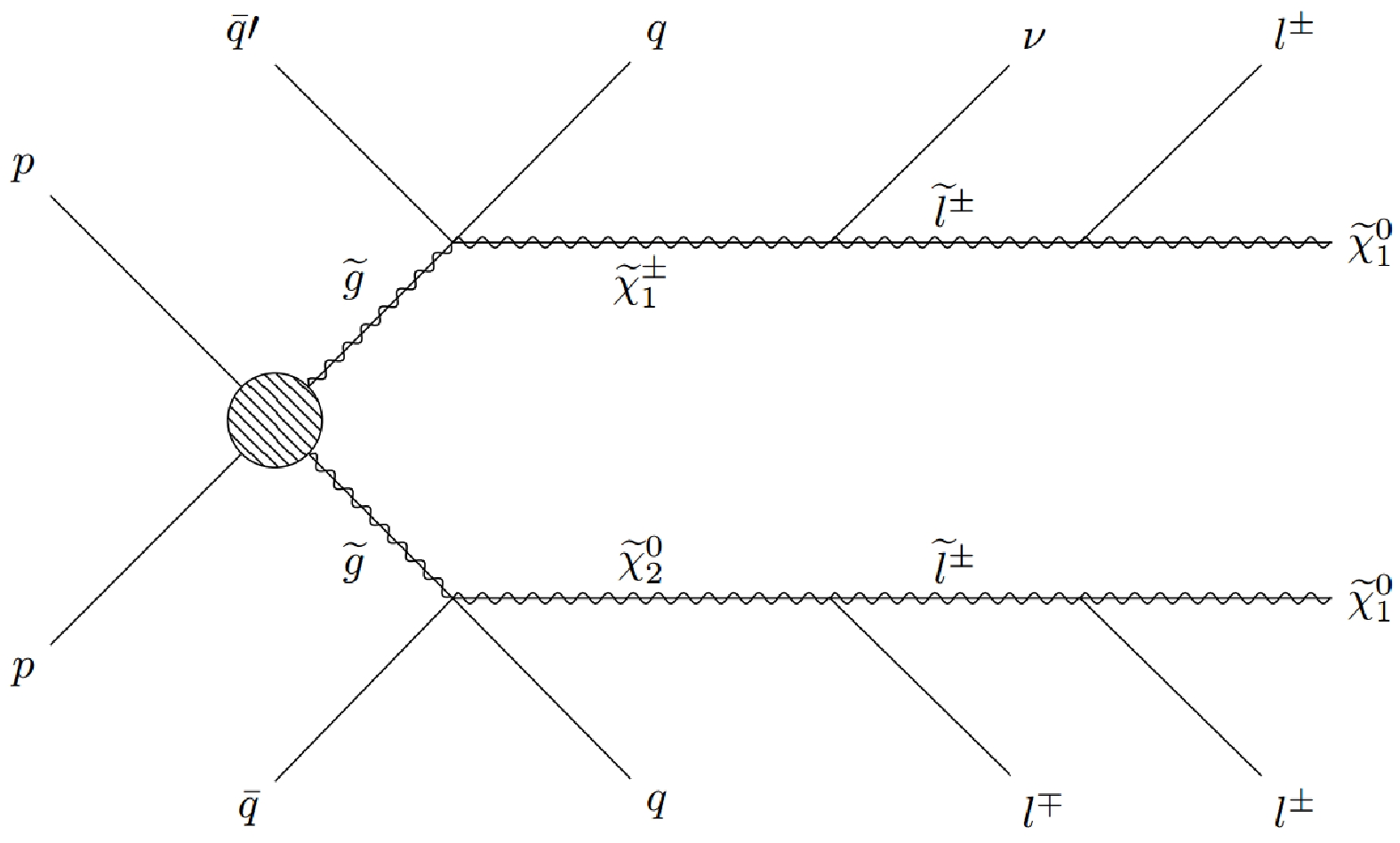

Figure 4.  Typical example of the decay topology of a gluino pair giving rise to the $ 3l+jets+{{\not {E_T}}} $ final state. It has been presented for illustrative purposes.

From the BR tables, we can see that many branches are required in the decay topology to obtain a higher lepton multiplicity (for example, $ 4l $, $ 5l $) in the models. These branches significantly reduce the overall probability of obtaining events consisting of multi-leptons, especially $ 5l $. This is why a detailed MVA cannot be conducted for the $ 5l $ signal. The insufficient number of events may lead to a statistically incorrect interpretation. Therefore, detailed analyses of our models in the context of the first three signal topologies are the primary focus of this study.

The traditional CCA provides first hand information on the significance of various signals against relevant backgrounds. Only events that pass the pre-selection cuts mentioned in Sec. III.C are considered for CCA. After data cleaning, we apply several suitable kinematic cuts to differentiate signal events from background ones depending on the desired final states composed of multiple leptons. We perform the CCA technique for the $ 2l $, $ 3l $, and $ 4l $ final states. However, we must briefly mention that the results obtained from CCA are not at all encouraging. Hence, we decide against discussing the details of the CCA results. For the purpose of illustration, we present the most promising results obtained for the $ 3l+jets+{{\not {E_T}}} $ final state in the following subsections.

In this subsection, we present the CCA results for the final state comprising $ 3l+jets+{{\not {E_T}}} $ at LHC RUN-III in the context of the various models described in Sec. II. The main SM backgrounds considered for this particular final state are $ t\bar{t} $, dibosons such as $ WZ $, $ ZZ $, tribosons such as $ WWW $, $ WWZ $, $ WZZ $, $ ZZZ $, as well as $ t\bar{t}Z $, $ t\bar{t}W $, $ t\bar{t}h $, $ hW $, and $ hZ $. To distinguish the signal from the SM backgrounds, we use appropriate kinematic variables to compute the significance using the traditional CCA method. Various kinematic variables and the corresponding selection cuts for BP1 (BP2) are mentioned below.

● Missing transverse energy ($ {{\not {E_T}}} $) : $ {{\not {E_T}}} > $ 150 (100) GeV

● The $ p_T $ of the leading lepton ($ p_T ^{l_1} $) : $ p_T ^{l_1}> $ 60 (25) GeV

● The $ p_T $ of the leading jet ($ p_T ^{j_1} $) : $ p_T ^{j_1}> $ 150 (100) GeV

● The transverse mass ($ m_T $) : $ m_T > $ 100 (100) GeV

● The scalar sum of the $ p_T $ of the three final state leptons ($ L_T $) : $ L_T> $ 150 (75) GeV

● Effective mass ($M_{\rm eff}$) : $M_{\rm eff} >$ 500 (250) GeV

One of the three leptons originating from the decay of the W boson for different SM backgrounds exhibits a Jacobian peak around $ M_{W}/2 $. Such backgrounds containing a W boson can be suppressed by applying a suitable cut on $ p_T $ of the leading lepton.

The variable ($ m_T $) is defined as

where $ p_T^l $ refers to the $ p_T $ of the lepton that is not part of the opposite sign (OS) lepton pair closest to the mass of the Z boson, and $ \Delta\Phi_{m_T} $ is the difference in the azimuthal angle between $\vec{p}_T^{\rm miss}$ and $ \vec{p}_T^{\; l} $. The SM backgrounds show a peak for the kinematic variable $ m_T $ around $ M_W $. By imposing a cut on $ m_T $ ($ m_T > 100 $ GeV), the backgrounds are reduced significantly.

The variable $ L_T $ is defined as

In this multi-lepton final state, the variable $ L_T $ is a good discriminator between the signal events and the corresponding SM background ones. This is because the magnitude of $ L_T $ obtained from this particular signal is remarkably different from that from the SM backgrounds.

The variable effective mass ($M_{\rm eff}$) is defined as

Effective mass is a good discriminator for isolating SUSY events from the corresponding backgrounds. Massive SUSY particles can produce jets and leptons with high $ p_T $ along with a massive LSP, which always produces a significant amount of transverse missing energy. Thus, their combination, known as effective mass, is strikingly different from the SM backgrounds. Hence, it helps us discriminate the signal from the potentially significant backgrounds.

The results of the traditional CCA for the final state comprising $ 3l+jets+{{\not {E_T}}} $ are presented in Table 8, which includes the normalized number of signal and background events with respect to an integrated luminosity of 139 $\rm fb^{-1}$. The signal significances are shown in the fourth and sixth columns of Table 8 for the LLRL and LLRH models, respectively.

The results shown in Table 8 reveal that a very high luminosity is required for 5σ discovery of this particular signal with the CCA method. We use suitable cuts on some kinematic variables to obtain these results. Furthermore, it is noted that a set of new cuts or variables can modify the CCA results. In Sec. V.B, we perform MVA with the same set of kinematic variables adopted in this subsection as the input features of the BDT to obtain a better significance, resulting in the requirement of a relatively low luminosity for the discovery of the gluino through this particular channel.

Here, an MVA approach is employed for improved signal-to-background differentiation, resulting in increased significance. The BDT algorithm for MVA is implemented in the TMVA framework within the ROOT platform. To improve the significance from the cut-based analysis previously discussed, finding an optimal cut value for the variables can be a challenging task using traditional rectangular cut methods. The MVA technique serves as a powerful tool for optimizing sensitivity for a given set of input features.

Opposite sign same flavor (OSSF) lepton

The signal comprising opposite sign same flavor (OSSF) dileptons along with jets and the missing transverse energy stems from the production of a pair of gluinos at the 13.6 TeV LHC. The potential SM backgrounds that can mimic the signal are $ t\bar{t} $ Drell-Yan, dibosons such as $ WW $, $ WZ $, and $ ZZ $, tribosons such as $ WWW $,$ WWZ $, $ WZZ $, and $ ZZZ $, as well as $ t\bar{t}Z $, $ t\bar{t}W $, $ t\bar{t}h $ , $ hW $, and $ hZ $.

We use five kinematic inputs as the features of the BDT classifier to distinguish the SM backgrounds from the corresponding SUSY signal. The features are given below.

● The $ p_T $ of the leading jet: $ p_T ^{j_1} $

● Missing transverse energy : $ {{\not {E_T}}} $

● The invariant mass of the two OSSF leptons :$ M_{LL} $

● The $ p_T $ of the leading lepton : $ p_T ^{l_1} $

● The scalar sum of the $ p_T $ of the two final state leptons : $ L_T $

● Effective mass : $ M_{\rm eff} $

In this study, we employ the basic kinematic variables mentioned above because they have less correlation and demonstrate a considerable power to distinguish the SUSY signal over the SM backgrounds. In Table 9, we provide these variables along with their method-specific ranking in the BDT response. This may vary slightly depending on the specific set of parameters corresponding to BP1 and BP2. The event distributions normalized to the luminosity are presented in Fig. 5. From Fig. 5, we can infer that altogether these five variables have a good amount of discriminating power. In Fig. 6, we present the receiver operating characteristic (ROC) curve. The area below the ROC curve provides a clear indication of the considerable separation between the signal and backgrounds and quantifies the combined performance of the BDT.

Variable	Variable importance
$M_{\rm eff}$	$ 2.514 \times 10^{-1} $
$ p_T^{j_1} $	$ 2.257 \times 10^{-1} $
$ p_T^{l_1} $	$ 1.801 \times 10^{-1} $
$ {{\not {E_T}}} $	$ 1.510 \times 10^{-1} $
$ L_T $	$ 1.249 \times 10^{-1} $
$ M_{LL} $	$ 6.687 \times 10^{-2} $

Table 9.  Method-specific ranking of the input features used in the BDT to discriminate the $ 2l+jets+{{\not {E_T}}} $final state with an opposite sign same flavor (OSSF) dilepton from the corresponding backgrounds.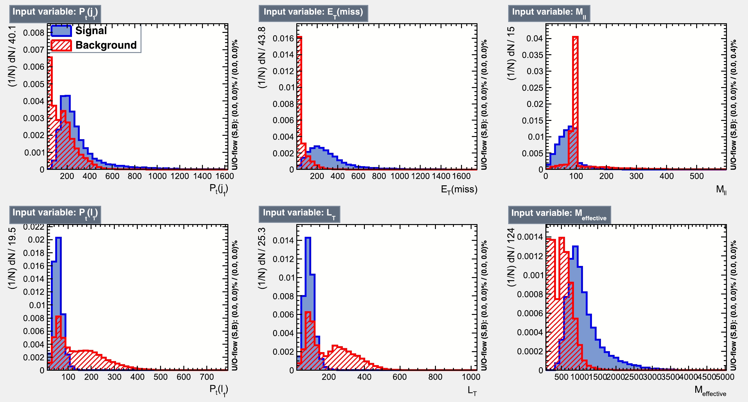

Figure 5.  (color online) Signal (blue) and background (red) distributions of the input features in the final state comprising $ 2l+jets+{{\not {E_T}}} $with an opposite sign same flavor (OSSF) dilepton corresponding to BP2 of the light electroweakino light slepton wino (LELSW) model in the left light and right heavy squark (LLRH) scenario.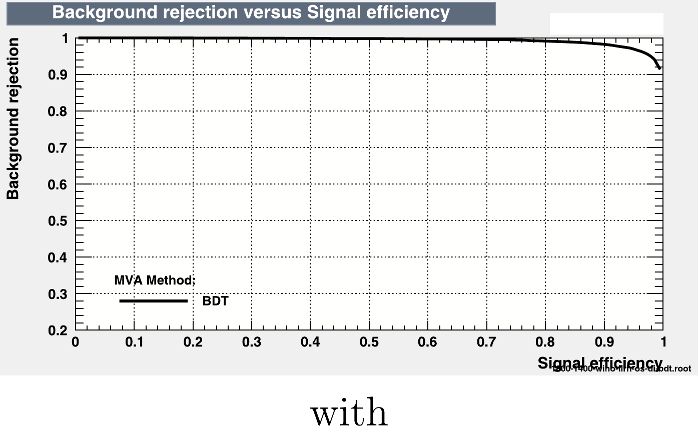

Figure 6.  (color online) ROC curve for the signal comprising $ 2l+jets+{{\not {E_T}}} $ with an opposite sign same flavor (OSSF) lepton pair corresponding to BP2 of the same model as in Fig. 5.

The Kolmogorov-Smirnov (KS) test can be used to check if a test sample is over-trained. Generally, a KS probability between 0.1 and 0.9 indicates that the test sample is not over-trained. A critical KS probability value greater than 0.01 confirms that the samples are not over-trained in most cases. Fig. 7, which shows the KS probability values for the signal and backgrounds of the BDT response, indicates that neither the signal nor the background samples are over-trained. As seen in Fig. 7, the signal and background samples in this BDT output are well-separated, enabling us to significantly enhance the signal significance by applying an appropriate BDT cut.

In Table 10, we present the yield of signal events and that of the background events for wino, higgsino, and wino-higgsino mixed (wiggsino) type models with two variants of each model, namely, LLRL and LLRH (see Sec. II). The BDT cut values for different models to discriminate signals over the backgrounds are shown in columns 3 and 7. The projected luminosities for the discovery of gluinos in terms of significances through this channel are presented in columns 6 and 10.

BP	Model	LLRL					LLRH
		BDT cut value	$N_S$	$N_B$	Required luminosity for discovery/fb−1		BDT cut value	$N_S$	$N_B$	Required luminosity for discovery/fb−1
BP1	LELSW	0.352	0.98	−	710		0.323	1.82	−	380
	Wiggsino	0.353	0.33	−	2110		0.345	0.73	−	950
	LELSH	0.314	0.21	−	3300		0.329	0.29	−	2380
BP2	LELSW	0.212	2.29	1.35	1320		0.225	1.91	0.26	640
	Wiggsino	0.224	0.41	−	1700		0.220	1.86	0.48	840
	LELSH	0.227	0.39	−	1750		0.256	0.72	−	965

Table 10.  Number of $ 2l+{{\not {E_T}}}+jets $ (OSSF) signal ($ N_S $) events and the corresponding cumulative background ($ N_B $) events after passing the BDT cut normalized to an integrated luminosity of 139 $\rm fb^{-1}$with a centre of mass energy of 13.6 TeV at the LHC. In addition, we consider a 10% systematic uncertainty on the overall backgrounds. Here, we also show the required luminosity to achieve a potential for discovery. "-" denotes the negligible background ($ N_B\rightarrow0 $) events compared to the signal events. In case the background is negligible, five signal events are considered as discovery criteria.

From the results, it is clear that for wino type models, the discovery prospect at LHC RUN-III is promising compared to that of other higgsino and wiggsino models because the former requires a low luminosity. This is because in wino type models, gluinos mostly decay into lighter eweakinos because they are wino dominated. Moreover, because sleptons are lighter than eweakinos, they further decay into either sleptons or sneutrinos with 100% BRs. This results in the final state being composed of two OSSF leptons, whereas in higgsino type scenarios, the gluinos decay into the heavier eweakinos (wino dominated) with a substantial amount of BRs (see Table 6). The heavier eweakinos further decay into an SM particle along with the LSP through a long cascade, resulting in a decrease in the probability of obtaining two leptons in the final state. However, for the mixed case, the results are intermediate between the two.

Moreover, when such models are subcategorized in terms of the squark mass hierarchy, namely, the LLRL and LLRH variants, the LLRH case is found to give the better significance across all classes of models. This is because if R-squarks are made heavier, the BR of gluinos into a bino-like LSP decreases and the BR of the chargino enhances, thereby increasing the strength of the $ 2l+jets+{{\not {E_T}}} $ signal. As a result, when observing the signal in the LLRH wino model, the requirement of integrated luminosity is always smaller compared to the other. The best result for this particular signal is obtained for BP1 in the wino type LLRH scenario because the required luminosity is approximately 380 $\rm fb^{-1}$, which may be achieved at an early stage of LHC RUN-III. However, there are other scenarios that can give hints of gluino discovery for relatively low luminosities.

For higgsino type models in the LLRH scenario, the BP2 corresponds to an integrated luminosity of 965 $\rm fb^{-1}$ for discovery, which may be a promising search channel to be probed at the early stage of HL-LHC.

Same sign same flavor (SSSF) dilepton

Here, we explore the potential for discovering gluinos in the final state consisting of a pair of SSSF leptons in association with jets and $ {{\not {E_T}}} $. The SM backgrounds for this final state are $ t\bar{t} $, dibosons such as $ WZ $, tribosons such as $ WWW $, $ WWZ $, $ WZZ $, as well as $ t\bar{t}Z $, $ t\bar{t}W $, and $ hW $. Here, the backgrounds are relatively weaker compared to those of the OSSF final states. Hence, the presence of SSSF lepton pairs from the Majorana fermions in the SUSY signal makes this search channel worth investigating.

The following four features considered in the previous search channel are used here to distinguish the required signal from the backgrounds. The four distinguishing features are given below.

● The $ p_T $ of the leading jet: $ p_T^ {j_1} $

● Missing transverse energy : $ {{\not {E_T}}} $

● The $ p_T $ of the leading lepton : $ p_T ^{l_1} $

● The scalar sum of the $ p_T $ of the two final state leptons : $ L_T $

● Effective mass : $M_{\rm eff}$

We present the importance of these variables in terms of their ranking in the BDT response in Table 11. The event distributions, normalized to the luminosity, are shown in Fig. 8. From this figure, we can see that these four variables possess a considerable amount of discriminating power.

Variable	Variable importance
$M_{\rm eff}$	$ 2.290 \times 10^{-1} $
$ {{\not {E_T}}} $	$ 2.105 \times 10^{-1} $
$ p_T ^{j_1} $	$ 1.966 \times 10^{-1} $
$ L_T $	$ 1.844 \times 10^{-1} $
$ p_T ^{l_1} $	$ 1.795 \times 10^{-1} $

Table 11.  Method-specific ranking of the input features used in the BDT to discriminate the$ 2l++jets+{{\not {E_T}}} $ SSSF final state.

Finally, to ensure that the classifier is not over-trained, we perform a KS test, which compares the BDT response curves of the training and testing sub-samples. From Fig. 9, we can infer that the response curves do not exhibit any significant over-training. Additionally, we present the ROC curve for this topology of the signal in Fig. 10.

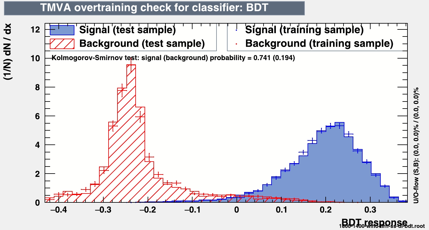
Figure 9.  (color online) For the purpose of illustration, we present the over-training check of the BDT response for the model mentioned in Fig. 5, with the final state comprising a same sign same flavor (SSSF) pair of leptons in the $ 2l+jets+{{\not {E_T}}} $ signal using the parameter set of BP2.

Figure 10.  (color online) ROC curve for the model mentioned in Fig. 5 corresponding to the final state comprising $2l+jets+ $$ {{\not {E_T}}}$ with an SSSF pair.

In Table 12, we show the normalized event number after passing the BDT cut value. From the table, we can infer that gluinos have the best discovery potential corresponding to an integrated luminosity of 490 $ fb^{-1} $ in the final state comprising $ 2l+jets+{{\not {E_T}}} $with a pair of SSSF leptons at the HL-LHC, corresponding to BP2 for the LLRH sub-variant of the LELSW model. This happens because the strength of the leptonic signal is greater for the LLRH sub-variant than the LLRL of the wino type model among all the models considered. Furthermore, owing to the greater OSSF leptonic signal for this particular signal, the prospect of the gluino is more promising than the corresponding SSSF signal, which is readily observable from Tables 10 and 12.

BP	Model	LLRL					LLRH
		BDT cut value	$N_S$	$N_B$	Required luminosity for discovery/fb−1		BDT cut value	$N_S$	$N_B$	Required luminosity for discovery/fb−1
BP1	LELSW	0.430	0.87	0.31	2430		0.471	0.31	−	2240
	Wiggsino	0.449	0.63	0.21	3300		0.436	1.48	2.10	4000
	LELSH	0.506	0.18	−	3860		0.548	0.23	−	3050
BP2	LELSW	0.227	3.10	5.93	2500		0.211	8.44	7.29	490
	Wiggsino	0.272	0.18	−	3860		0.220	3.21	2.68	1230
	LELSH	0.243	0.03	−	– –		0.238	0.85	2.14	– –

Table 12.  Number of $ 2l+jets+{{\not {E_T}}} $ (SSSF) signal ($ N_S $) and corresponding cumulative background ($ N_B $) events after passing the BDT cut normalized to an integrated luminosity of 139$\rm fb^{-1}$with a centre of mass energy of 13.6 TeV at the LHC. In addition, we consider a 10% systematic uncertainty on the overall backgrounds. In this table, we also show the required luminosity to achieve a potential for discovery. "- " denotes the negligible background ($ N_B\rightarrow0 $) compared to the signal. In case the background is negligible, five signal events are considered as the requirement for the discovery. "$--$" denotes that the required luminosity is equal or higher than 5000 $\rm fb^{-1}$, and hence the prospect of gluino discovery even in the HL-LHC is not optimistic for these BPs.

The pair production of strongly interacting gluinos can result in a final state containing the $ 3l+jets+{{\not {E_T}}} $ signature in various models described in Sec. II at LHC RUN-III. The important SM backgrounds for this particular decay topology are mentioned in Sec. V.A.1.

In this subsection, we also use five simple kinematic features in the BDT to discriminate the signal from the SM backgrounds. The features are

● The $ p_T $ of the leading jet: $ p_T ^{j_1} $

● Missing transverse energy : $ {{\not {E_T}}} $

● The transverse mass : $ m_T $

The variable ($ m_T $) is defined as $ m_T = $ $\sqrt{2 p_T^{\rm miss} p_T^l [1- \cos(\Delta\Phi_{m_T})]}$, where $ p_T^l $ refers to the $ p_T $ of the lepton that is not part of the OS pair closest to the Z boson mass, and $ \Delta\Phi_{m_T} $ is the difference in azimuth angle between the missing transverse momentum ($\vec{p}_T^{\,\rm miss}$) and $ \vec{p}_T^{\; l} $.

● The $ p_T $ of the leading lepton : $ p_T ^{l_1} $

● The scalar sum of the $ p_T $ of the three final state leptons : $ L_T $

● Effective mass : $M_{\rm eff}$

In addition to the four features used in the last subsection, we consider the transverse mass as the distinguishing feature to significantly tame the potential backgrounds. It is further noted from Fig. 11 that the transverse mass feature has a significant power to differentiate the signal from large SM backgrounds containing the W boson.

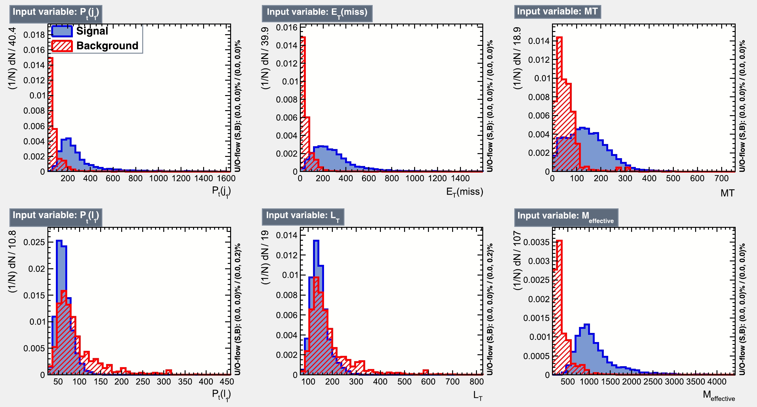
Figure 11.  (color online) Signal (blue) and background (red) distributions of the input features in the final state comprising $ 3l+jets+{{\not {E_T}}} $, corresponding to BP2 of the light electroweakino light slepton wino model (LELSW) where R-squarks are heavy (LLRH).

From Table 13, where we present the method specific variable importance in the BDT output response, it can easily be seen that these features have remarkable importance in identifying the signal. Additionally, in Fig. 11, we present the distribution of the weighted number of the signal and background events against each feature used here. Next, to check whether the classifier is over-trained, we perform the KS test, which compares the BDT response curves of the training and testing sub samples, as seen in Fig. 12. The response curves are well within the tolerance of over-training. In addition to the KS test, we present the ROC curve in Fig. 13 for this decay topology. The area under the ROC curve shows that the chosen features are altogether good discriminators of the signal and SM backgrounds.

Variable	Variable importance
$M_{\rm eff}$	$ 1.929 \times 10^{-1} $
$ m_{T} $	$ 1.737 \times 10^{-1} $
$ p_T^{l_1} $	$ 1.647 \times 10^{-1} $
$ {{\not {E_T}}} $	$ 1.610 \times 10^{-1} $
$ L_T $	$ 1.579 \times 10^{-1} $
$ p_T^{j_1} $	$ 1.498 \times 10^{-1} $

Table 13.  Method-specific ranking of the input features used in the BDT to discriminate the$ 3l+{{\not {E_T}}}+jets $ final state.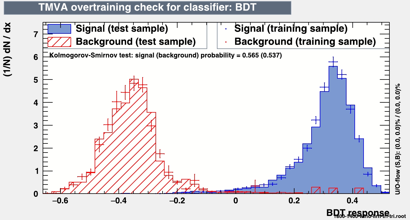

Figure 12.  (color online) For the purpose of illustration, we present the over-training check of the BDT response for the model mentioned in Fig. 11, with the final state comprising the $ 3l+jets+{{\not {E_T}}} $ signal using the parameter set of BP2.

Table 14 displays the number of signal and background events in response to the classifier cut value. The description of the table is as described in the previous section. Now, we discuss the important results obtained in this analysis.

BP	Model	LLRL					LLRH
		BDT cut value	$N_S$	$N_B$	Required luminosity for discovery/fb−1		BDT cut value	$N_S$	$N_B$	Required luminosity for discovery/fb−1
BP1	LELSW	0.429	0.61	0.11	2550		0.401	1.06	0.33	1855
	Wiggsino	0.488	0.52	0.18	3850		0.455	0.90	0.21	2050
	LELSH	0.345	0.46	0.11	3550		0.411	0.68	0.18	2600
BP2	LELSW	0.344	2.30	0.59	720		0.270	7.46	2.34	270
	Wiggsino	0.356	0.21	−	3310		0.226	4.45	1.56	480
	LELSH	0.379	0.28	−	2480		0.247	1.76	1.38	2090

Table 14.  Number of $ 3l+jets+{{\not {E_T}}} $ signal ($ N_S $) and corresponding cumulative background ($ N_B $) events after passing the BDT cut normalized to an integrated luminosity of 139$\rm fb^{-1}$with a centre of mass energy of 13.6 TeV at the LHC. In addition, we considered a 10% systematic uncertainty on the overall backgrounds. In this table, we also show the required luminosity to achieve a potential for discovery. "-" denotes the negligible background ($ N_B\rightarrow0 $) compared to the signal. In case the background is negligible, five signal events are considered as a requirement for the discovery.

BP2, corresponding to a lighter gluino mass, has a larger production cross section compared to BP1. From the table, it is observed that wino type models are more promising than other models in terms of the discovery prospects of the gluino.

A three lepton signal can primarily arise from gluinos decaying into lighter charginos and the second lightest neutralino, leading to a final state comprising three leptons in the wino type scenario. In other models (for example, the higgsino type), the three lepton signal may originate from the decays of heavier eweakinos. However, the probability of obtaining this signal is small because the leptons arise through long cascades, resulting in a decrease in the signal strength. Hence, the luminosity requirement for the observability of the signal is high for such models compared to that in wino type models.

It is further noticed from Table 14 that for BP2 in the LLRH model, even for a 270 fb$ ^{-1} $luminosity, the signal reaches the 5σ discovery limit. This is the best probe for gluino searches at HL-LHC, which corresponds to the lowest integrated luminosity. The LLRL models correspond to high luminosity compared to LLRH models for the discovery prospects, as discussed in Sec. V.B.1. Furthermore, owing to the low SM backgrounds for this signal topology, the significance is greater, resulting in a lower required luminosity compared to the signal comprising $ 2l+jets+{{\not {E_T}}} $.

Gluinos can be probed through the $ 4l+jets+{{\not {E_T}}} $ channel by reducing the backgrounds to a negligibly small level using the MVA technique. The cascade decay of heavier eweakinos leading to a signal comprising $ 4l+{{\not {E_T}}}+jets $ causes the signal strength to be weaker than that of the other signatures discussed previously. For the four lepton final state, the dominant backgrounds from the SM are processes involving three or two vector bosons, such as $ ZZ $, $ ZZZ $, $ WZZ $, $ WWZ $, top quark pair production in association with a Z boson $ (t\bar{t}Z) $, top quark production in association with a Higgs boson $ (t\bar{t}h) $, and Higgs boson production in association with a Z boson $ (hZ) $. The five kinematic variables used as the input features of the BDT are

● The $ p_T $ of the leading jet: $ p_T^{j_1} $

● Missing energy : $ {{\not {E_T}}} $

● The invariant mass of the four leptons : $ M_{4L} $

● The $ p_T $ of the leading lepton : $ p_T^{l_1} $

● The scalar sum of the $ P_T $ of the four final state leptons : $ L_T $

● Effective mass : $M_{\rm eff}$

The method-specific variable importance is presented in Table 15 for the five input features mentioned above. Furthermore, in Fig. 14, we show the distribution of the number of signal and background events against each feature used, with appropriate weightage. A KS test is performed to ensure that the classifier is not overtrained. This test compares the response curves of the BDT for the training and testing sub-samples, as shown in Fig. 15. These response curves shows that there is no significant over-training, and the classifier is able to effectively differentiate between the signal and backgrounds. In addition, we present the ROC curve in Fig. 16 for this decay topology.

Variable	Variable importance
$M_{\rm eff}$	$ 2.377 \times 10^{-1} $
$ p_T^{l_1} $	$ 1.682 \times 10^{-1} $
$ L_T $	$ 1.634 \times 10^{-1} $
$ {{\not {E_T}}} $	$ 1.593 \times 10^{-1} $
$ M_{4l} $	$ 1.430 \times 10^{-1} $
$ p_T^{j_1} $	$ 1.284 \times 10^{-1} $

Table 15.  Method-specific ranking of the input features used in the BDT to discriminate the $ 4l+jets+{{\not {E_T}}} $ final state.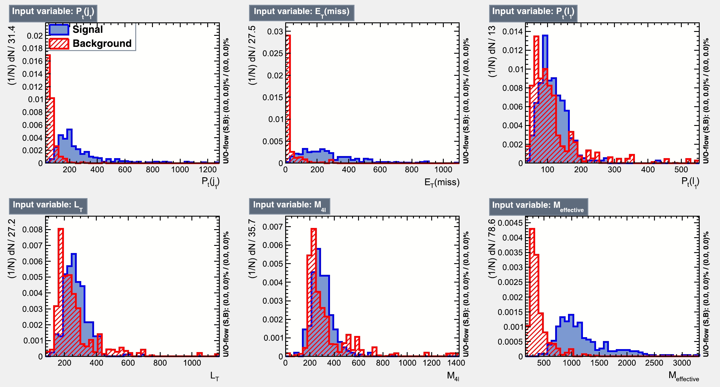

Figure 14.  (color online) Signal (blue) and background (red) distributions of the input features in the final state comprising $ 4l+jets+{{\not {E_T}}} $, corresponding to BP2 of the wino higgsino mixed type model (WIGGSINO) in the left light and right heavy squark (LLRH) scenario.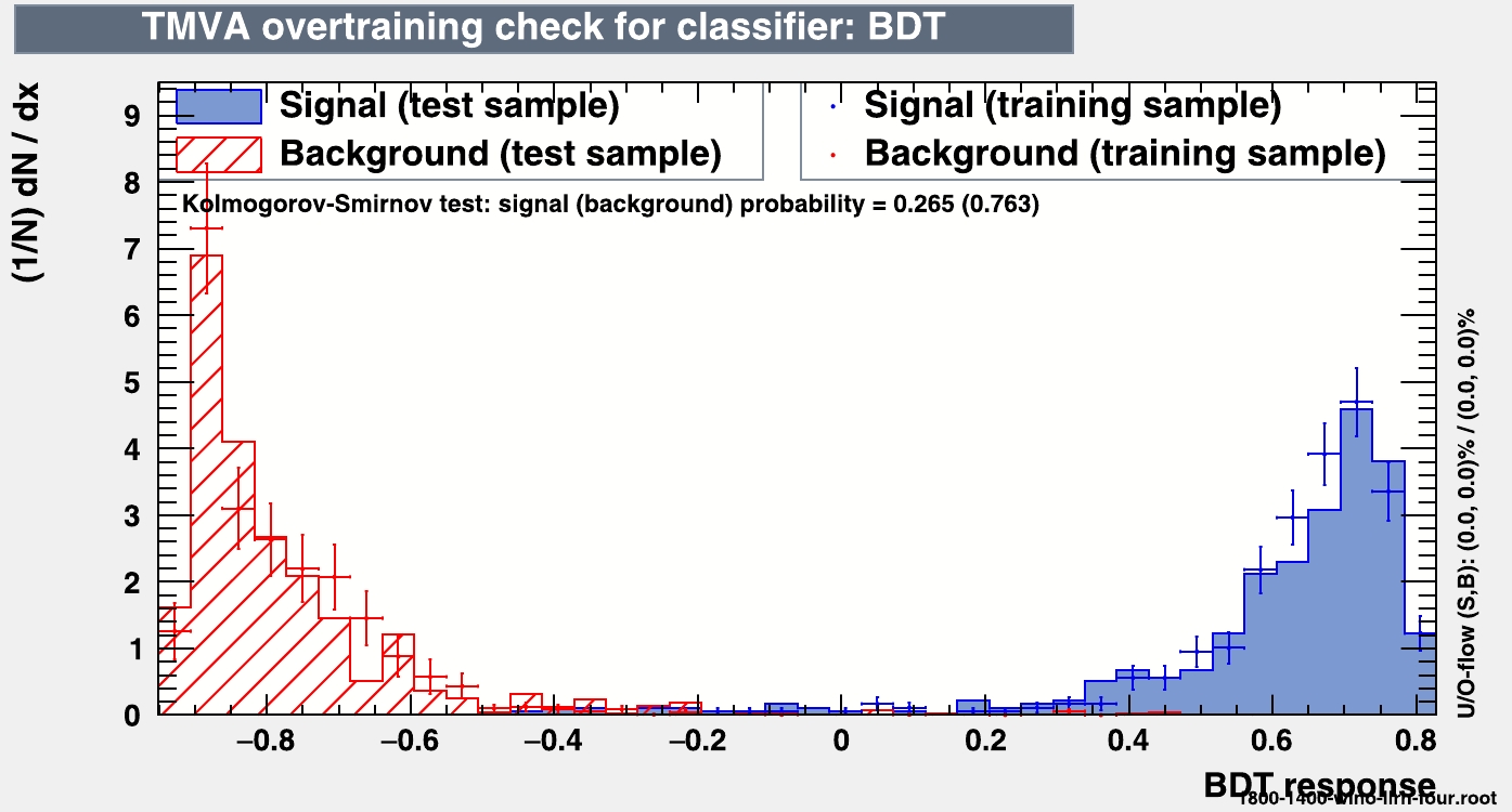

Figure 15.  (color online) For the purpose of illustration, we present the over-training check of the BDT response for the model mentioned in Fig. 14, with the final state comprising the $ 4l+jets+{{\not {E_T}}} $ signal using the parameter set of BP1.

Table 16 shows the number of events for the signal and backgrounds after applying the classifier specific optimised cut value. Two sets of BPs for various pMSSM scenarios are displayed in the table.

BP	Model	LLRL					LLRH
		BDT cut value	$N_S$	$N_B$	Required luminosity for discovery/fb−1		BDT cut value	$N_S$	$N_B$	Required luminosity for discovery/fb−1
BP1	LELSW	0.205	0.06	−	− −		0.293	0.11	−	− −
	Wiggsino	0.303	0.06	−	− −		0.242	0.10	−	− −
	LELSH	0.235	0.08	−	− −		0.293	0.11	−	− −
BP2	LELSW	0.301	0.33	0.02	2580		0.248	0.90	13	1350
	Wiggsino	0.334	0.08	0.02	− −		0.391	0.39	−	1780
	LELSH	0.628	0.13	−	− −		0.548	0.44	−	1580

Table 16.  Numbers of $ 4l+jets+{{\not {E_T}}} $ signal ($ N_S $) and corresponding cumulative background ($ N_B $) events after passing the BDT cut normalized to an integrated luminosity of 139$\rm fb^{-1}$with a centre of mass energy of 13.6 TeV at the LHC. In addition, we consider a 10% systematic uncertainty on the overall backgrounds. In this table, we also show the required luminosity to achieve a potential for discovery. "-" denotes the negligible background ($ N_B\rightarrow0 $) compared to the signal. In case the background is negligible, five signal events are considered as the requirement for the discovery. These numbers are normalized to a luminosity of 139 $\rm fb^{-1}$. "$- -$" denotes that the required luminosity is equal or higher than 5000 $\rm fb^{-1}$, and hence the prospect of gluino discovery even in the HL-LHC is not optimistic for these scenarios.

As shown in Table 16, BP2 corresponding to LLRL and LLRH of the wino like scenario and LLRH of the higgsino like scenario can be probed in the ongoing HL-LHC. In all the cases, the backgrounds being vanishingly small, only five signal events are considered as discovery criteria. For BP2 in the LLRH higgsino type model, the required luminosity is 1580 $\rm fb^{-1}$, which is expected to be achieved in the ongoing LHC RUN-III operation. However, for this particular signal, the BP2 corresponding to the wino type scenario for the LLRH case, the required luminosity is the least, at 1350 $\rm fb^{-1}$. Comparing Tables 10, 12, 14, and 16, we can observe that to probe gluino searches in higgsino type models, the required luminosity is the least, corresponding to the $ 4l+jets+{{\not {E_T}}} $ signal. The results show that the $ 4l+jets+{{\not {E_T}}} $ signal significance is smaller than the other signal topologies considered. This is due to the small BRs of gluinos decaying into the final state comprising the $ 4l+jets+{{\not {E_T}}} $ signal in wino type models. The same occurs for the other models discussed here due to the long cascade decay.

We explore the possibility of probing the strong sector of SUSY through gluino searches in different channels with multiple leptons in various pMSSM scenarios at the ongoing LHC RUN-III experiment with a center-of-mass energy of 13.6 TeV. This study provides the first results on gluino searches through multi-lepton channels at the most recent and, possibly, highest center-of-mass energy of the LHC to date.

All the BPs considered in this study are consistent with the LHC RUN-II data. We also consider other low energy observables such as the relic density of SUSY dark matter (the lightest neutralino) and the anomalous magnetic moment of muons. The BPs lie well within the$ 4\sigma $ range about the experimentally quoted central value of $ (g-2)_{\mu} $. However, in most of the pMSSM scenarios, the BPs satisfy the PLANCK/WMAP data.

In Sec. II, we primarily define three different models in the pMSSM framework based on different compositions of gaugino and higgsino components in eweakinos. Moreover, these models can be dissected further in terms of L- and R-type squarks and their mass hierarchy. In addition, slepton masses are set at values less than eweakinos masses. Such mass hierarchies are required to achieve multi-lepton final states from gluino pair production. Instead of conventional multijet and one/two lepton searches for supersymmetric gluinos, we try to put forward a proposition where multi-lepton ($ \ge 2 $ leptons) searches can become a potential discovery channel at LHC RUN-III.

First, we discuss the traditional CCA in Sec. V.A, where the results corresponding to the signal $ 3l+jets+{{\not {E_T}}} $ are displayed in Table 8. Because the CCA method does not exhibit a statistically significant surplus of events compared to the SM prediction, we take recourse to the MVA technique. In Sec. V.B, we present the results of the MVA.

We use the MVA technique with a BDT as the classifier to discriminate signal events from background events.The important kinematic variables chosen as features for discriminating between the signal and background are shown in Tables 9, 11, 13, and 15. The ROC curves are also displayed to establish the sanctity of the results. The results of the BDT analysis are summarized in Tables 10, 12, 14, and 16.

Although we consider two BPs satisfying the ATLAS data [54−56], the conclusions drawn in this study through multi lepton channels of gluino searches over the region of parameter space in between these BPs do not change. The first BP is chosen in such a way that the gluino mass is higher ($ \simeq 2.3 $ TeV) and the LSP is lighter. This choice allows for a relaxed kinematic phase space including other sparticles in between the gluino and the LSP. However, the gluino pair production cross section in this case is relatively smaller due to the heavier mass.

On the other hand, the second BP is located in a more compressed region, where the mass difference between the gluino and the LSP is only approximately $ 400 $ GeV, with the other sparticles packed in between. In this case, the cross section for gluino pair production is larger than that of the first BP because the gluino mass in this case is considerably smaller. However, the mass splitting is small, which results in a smaller cut efficiency.

In our decay topology, the inclusion of sleptons and other heavier eweakinos leads to a final state rich in leptons, making it observable in the upcoming LHC RUN III. By analyzing these BPs, we can gain insight into the discovery potential of the gluino between these two points. The interplay between the cut efficiency and the cross section makes for an interesting study. The result can be generalized for parameter space points in between these two extreme BPs.

Some important findings of this study are summarized below.

● The most encouraging result is that there is a possibility of observing the $ 3l+jets+{{\not {E_T}}} $ signal with $ 5\sigma $ significance at an integrated luminosity of 270 fb$ ^{-1} $ at LHC RUN-III, which can potentially originate from a pair of gluinos with $ M_{\tilde{g}} \approx 1.8 $ TeV corresponding to the wino type model in the LLRH case.

● LHC RUN-III also has the potential to discover a gluino of mass $ 2.3 $ TeV in the same wino type model in the LLRH case in a two OSSF lepton $ +jets+{{\not {E_T}}} $ final state after collecting and analysing 380 fb$ ^{-1} $ data.

● Same sign dilepton signals are usually considered propitious search channels, particularly at hadron colliders. However, in the SSSF dilepton$ +jets+ {{\not {E_T}}} $ final state, LHC RUN-III requires the collection of 490 fb$ ^{-1} $ data to reach the discovery significance for a gluino with a mass of approximately 1.8 TeV in the wino type model in the LLRH case.

● On the other hand, observing signals in higgsino type models is rather challenging. A luminosity of 965 fb$ ^{-1} $ is required for LHC RUN-III to claim discovery of a gluino with a mass of 1.8 TeV in the OSSF dilepton+ jets+$ {{\not {E_T}}} $ final state.

● Final states with lepton multiplicities greater than three, however, reduce the signal significance considerably, although the corresponding backgrounds are vanishingly small. For example, for the $ 4l+jets+{{\not {E_T}}} $ signal originating from a gluino pair with $ M_{\tilde{g}}\approx 1.8 $ TeV, corresponding to the wino type scenario for the LLRH case, the required luminosity is 1350 $\rm fb^{-1}$. The situation for the remaining scenarios requires the HL-LHC.

In summary, the LLRH wino-type model in the pMSSM offers the most encouraging route to discover gluinos, requiring the lowest integrated luminosity expected to be obtained at an early stage of LHC RUN-III. This model resembles the simplified model that the ATLAS collaboration normally examines. The crucial factor is to include sleptons and all other eweakinos in the gluino decay chain, resulting in an enhancement in the multi-lepton signal in the final state. The analysis performed in this study is generic and can therefore be employed in similar types of BSM scenarios. We hope that following our direction of analysis, particularly the MVA technique for such multi-lepton final states, the ongoing run of the LHC shall be able to resolve this long-standing impasse in particle physics.

Abhi Mukherjee would like to acknowledge DST for offering the INSPIRE Fellowship [IF170693]. Jyoti Prasad Saha would like to thank the University of Kalyani for providing a personal research grant (PRG) to conduct research.